robust feature tracking in image sequences using view ... - ISPRS Annals

ISPRS Annals of the Photogrammetry, Remote Sensing and Spatial Information Sciences, Volume II-3/W2, 2013 ISA13 - The ISPRS Workshop on Image Sequence Analysis 2013, 11 November 2013, Antalya, Turkey

ROBUST FEATURE TRACKING IN IMAGE SEQUENCES USING VIEW GEOMETRIC CONSTRAINTS J. Lawver, A. Yilmaz

The Ohio State University Photogrammetric Computer Vision Laboratory 2070 Neil Ave., Columbus, OH 43210, United States ([email protected], [email protected]) Commission III, WG III/3

KEY WORDS: Object Tracking, Occlusion, Interest points, Scene Geometry

ABSTRACT: Interest point tracking across a sequence of images is a fundamental technique for determining scene motion characteristics. Traditionally, feature tracking has been performed with a variety of appearance-based comparison methods. The most common methods analyze intensity values of local pixels and subsequently attempt to match them to the most similar region in the following frame. This standard, though sometimes effective, lacks versatility. For example, these methods are easily confused by shadows, patterns, feature occlusion, and a variety of other appearance-based anomalies. To counteract the issues presented by a one-sided approach, a new method has been developed to take advantage of both appearance and geometric constraints in a complementary fashion. Using an iterative scheme, camera parameters are computed at each new frame and used to project a derived shape to new point coordinates. This process is repeated for each new frame until a trajectory is created for the entire video sequence. With this method, weight can be allocated as desired between both appearance and geometric constraints. If an issue arises with one constraint (e.g., occlusion or rapid camera movement), the other constraint will continue to track the feature successfully. Experimental results have shown that this method is robust to tracking challenges such as occlusion, shadows, and repeating patterns, while also outperforming appearance-based methods in tracking quality.

1. INTRODUCTION Ongoing advances in automated video analysis, as well as modern accessibility to high quality and affordable cameras and computers, has made object tracking an increasingly important task in the field of computer vision. There are a multitude of applications beginning to incorporate this analysis, including motion-based recognition, automated surveillance, humancomputer interaction, and video indexing, among many others (Yilmaz et al. 2006). However, determining motion information from image projections is a complex problem. Many natural occurring phenomena, such as 3D to 2D projec- tion information loss, image noise, complex object motion and shapes, non-rigid objects, object occlusion, and variable scene illumination cause significant difficulty in this domain (Yilmaz et al. 2006). Until recently, tracking has been performed exclusively using appearance-based matching techniques. The most common approach, template matching, involves extracting a neighborhood of intensity values around each feature point and subsequently attempting to locate the matching template in the following frame. This process assumes that the patch of pixels will appear similar from frame to frame, which is not often the case (Schweitzer et al., 2002). In other approaches, tracking is performed by using deterministic or stochastic motion models that utilize motion heuristics such as velocity, acceleration, proximity, rigidity, and common motion (Hue et al., 2002; Shafique and M. Shah, 2003). These approaches, much like template matching, are greedy and often struggle with noise and general uncertainty in the images.

1.1 Optical Flow As opposed to correspondence based approaches, optical flow is a method that handles object tracking as an iterative estimate and update to a feature’s motion. This method is used to construct the appearance constraint in the proposed algorithm. Assuming that a point’s appearance in one image remains constant to another image, any point can be represented by the brightness constancy equation (Beauchemin and Barron, 1995; Fleet et al., 2006)





Another assumption can be made that the movement of any given point is small from one image to the next, thus allowing a Taylor series expansion of the previous equation:





This shows that the partial derivatives are equal to zero:





Thus, each term can be divided by Δt to get the optical flow equation for any given point:







This contribution has been peer-reviewed. The double-blind peer-review was conducted on the basis of the full paper.



25

ISPRS Annals of the Photogrammetry, Remote Sensing and Spatial Information Sciences, Volume II-3/W2, 2013 ISA13 - The ISPRS Workshop on Image Sequence Analysis 2013, 11 November 2013, Antalya, Turkey This formulation is known as the optical flow equation, and is used to determine the displacements u and v of feature points moving through the scene. However, this equation cannot be solved independently since two unknowns exist. To solve for the displacement, a final assumption is introduced that states that neighboring pixels move with a common displacement. Thus, neighboring points can each introduce a unique optical flow equation with the same unknowns, allowing for a tracking solution determination using a least squares adjustment. This method is referred to as the Lucas-Kanade approach, a model later extended by Tomasi and Kanade to create the KLT tracker (Lucas and Kanade, 1981; Tomasi and Kanade, 1991).

scheme concludes, the resulting u and v represent the optical flow displacements for a given feature. In the proposed method, the Horn-Schunck method is used in conjunction with the Lucas-Kanade method to take advantage of the benefits of each. First, a geometrically-constrained LucasKanade approach is used to determine the smoothing constraints, ̅ and ̅ . These constraints are then added to the Horn-Schunck equations and solved iteratively, thus restricting the optical flow displacements to the defined geometry of the scene. Whereas the Horn-Schunck smoothing constrains the movement to the 2D scene geometry, the proposed method uses the same constraint in a higher dimensional perspective space. 1.2 Structure From Motion

Similar to the Lucas-Kanade approach, the Horn-Schunck method provides a more advanced technique for computing optical flow. In this method, all pixels are assumed to have approximately the same displacement vectors as their nearest neighbors, an assumption that suggests a global smoothing over the displacements in the image. To minimize the distortion in flow, Horn and Schunck attempt to minimize a global cost function defined by every pixel in the image. The first part of the cost function, ec, is defined globally using the optical flow parameters:







 

∬



A smoothness constraint is then introduced using the cost function es, which assumes that neighboring points have a similar displacement.



∬

 

∬



The two defined cost functions can be joined together using a Lagrange multiplier, �. By using the two cost functions together, flow is determined globally by ec while being simultaneously constrained in a local neighborhood by es.





∬[

]



This function is further minimized using the Euler-Lagrange equations and rearranged as an iterative scheme to allow for the displacements u and v to be solved locally for each iteration k.

̅ ̅

̅

̅

̅

̅









In both optical flow estimations, the equations are solved iteratively until It, the change in feature appearance between two time instances, converges near zero. When this iterative

The asset that differentiates the proposed method from others is the addition of a geometric constraint. While the tracking still relies on a feature’s appearance in the scene, it is also dependent on how a feature lies on an object in a higher dimensional subspace. Structure from motion, a method created to derive the shape of objects from corresponding points in stereo images, is used to determine this geometric structure. If relative translational movement exists between the camera and the scene through time, structure from motion (much like the human eye) is able to determine the feature depth (Shapiro and Stockman, 2001). The method used in this research for determining object shape from motion is known as the Tomasi-Kanade factorization method (Tomasi and Kanade, 1992). The first step to any structure from motion technique is acquiring point correspondence between the frames in the sequence. This can be done manually, though it is typically achieved with the help of a point tracking algorithm. Given N tracked feature points through M frames, a trajectory matrix T of size 2MxN is formed. In this matrix, the columns correspond to each feature point and the rows correspond to the tracked two-dimensional [ ] coordinates in each frame. To reduce calculation error in the factorization, the points in each frame are first mean-normalized such that their centroid lies at the image origin, resulting in the normalized matrix ̃ . Assuming that 2M ≥ N, ̃ can be decomposed using a singularvalue decomposition into a 2Mx2M matrix U, a 2MxN matrix S, and an NxN matrix V such that ̃ . The U and V matrices correspond to the left and right eigenvectors of ̃ , whereas the eigenvalues lie along the diagonal in S in decreasing order. The factorization method describes that some linear combination of these three matrices will provide the desired projection P and shape information X. If the goal of this research were to fully recover the structure from motion for reconstruction purposes, more steps would follow in the factorization. In tracking, however, the uniqueness of P and X is unimportant. The goal of tracking is to determine image coordinates, which are computed as the multiplicative projection of the two matrices. Thus, as long as the multiplication of P and X provide ̃ , the individual values of P and X are of no concern. In other words, any arbitrary homography transformation H satisfies the following equation:

̃



This contribution has been peer-reviewed. The double-blind peer-review was conducted on the basis of the full paper.



26

ISPRS Annals of the Photogrammetry, Remote Sensing and Spatial Information Sciences, Volume II-3/W2, 2013 ISA13 - The ISPRS Workshop on Image Sequence Analysis 2013, 11 November 2013, Antalya, Turkey Thus, there is no unique solution for P and X with regard to the tracking domain. This concept suggests that any shape matrix X that can be computed using the decomposed matrices lies in a subspace with all other possible X matrices. Specifically, any X defining object shape is related to any other X through a homographic transformation. Since ̃ is equal to , it is clear that some linear combination of the three decomposed matrices U, S, and V will equal P and X. As demonstrated above, as long as their product remains ̃ , the actual values for P and X are irrelevant for tracking exercises. Therefore, for this research the ̃ is factorized into P and X as follows:

̃



typical, such that KLT will discard any points with less than 99% accuracy confidence. This ensures that the points used in the factorization are correctly registered as to not skew the initial geometric constraints in the tracking model. Second, the amount of frames tracked by KLT is limited to the least possible as can be afforded without sacrificing sufficient parallax for an accurate geometric determination. Once the correspondences are determined for a subset of images, the geometric components can be determined using the Tomasi-Kanade factorization detailed in equations (14-18). With P and X computed, the 2D tracked points x at any future frame F can be found by solving:







 



In these equations, P is a 2MxN matrix consisting of each frame’s 2xN projection matrix, and X is a 2MxN matrix consisting of each feature point’s 2Mx1 geometric shape. Since the proposed method is tracking using geometric properties in the perspective domain, six eigenvalues are necessary to achieve tracking accuracy without introducing high-dimensional noise. To reduce to six eigenvalues, such that P is 2Mx6 and X is 6xN, only the eigenvectors up to rank-6 are used in determining P and X:



 



The calculated P and X values represent the relative camera projection and object shape in the scene. As long as objects in the scene remain static, the original trajectory T can always be recovered without loss by multiplying and de-normalizing with . This knowledge defines the constant geometry that is used to provide a geometric constraint for the proposed tracking algorithm. 2. TRACKING MODEL For optimal results, all sequences of images used in this research were converted to grayscale and smoothed using a 5x5 Gaussian filter with a sigma equal to one. Additionally, it’s computationally more efficient to compute and store image gradients prior to tracking, such that they are not recomputed in each iteration. Given the pre-processed images, a sub-pixel implementation of the Harris interest point detector is used to find the optimal features to track in the sequence. In order to complete the factorization, the corresponding points on a subset of images must be found using an interest point tracker. In this research the KLT tracker, based on the Lucas-Kanade optical flow method, is used. It should be noted that the reliance on KLT is a significant caveat in the proposed tracking method. In order to determine geometric constraints for the algorithm, it must first rely on the tracking of an appearance-based method. It is already well documented that appearance-based methods struggle in many scenarios, so it is a burden that KLT must be relied upon.



In this equation, the unknowns are , , and . The variables and refer to the change in projection matrix and mean, respectively, between frame 1 and the current frame F. Thus, the overlying goal of the tracking algorithm is to use the geometrically-constrained optical flow equations to compute these variables at each frame, thus allowing to be computed. 2.1 Iterative Tracking Model The proposed tracking algorithm is a combined approach consisting of components from both structure from motion and the Lucas-Kanade and Horn-Schunck optical flow algorithms. The underlying foundation is the optical flow equation (5). This equation can be rewritten to separate the two images undergoing tracking.

[

][ ]

[



][ ]



The subscript i refers to the previous frame and the subscript j refers to the current frame being tracked to. The unknowns in this equation are the coordinates in frame j. Rather than directly solving for these unknowns (e.g. Lucas-Kanade), they are instead replaced with the previously derived projection.

[

](

)

[



][ ]



The shape matrix X for the static points is a known constant. The matrix Pj is an unknown projection matrix to project X to the normalized point coordinates in frame j. The values in define an unknown mean to shift the resulting normalized points to their correct image locations. These unknowns can then be separated such that they represent incremental updates to previously defined variables at each frame. At iteration k, the equation to be solved is as follows.

[

] 

][ [



][ ]

This equation is rearranged such that the unknowns can be determined using a least squares direct solution. [ 

]



To partially counteract these issues, two securities are used. First, the threshold for KLT is set substantially higher than

This contribution has been peer-reviewed. The double-blind peer-review was conducted on the basis of the full paper.

27

ISPRS Annals of the Photogrammetry, Remote Sensing and Spatial Information Sciences, Volume II-3/W2, 2013 ISA13 - The ISPRS Workshop on Image Sequence Analysis 2013, 11 November 2013, Antalya, Turkey

]

[

[



]



As is, this formulation is only a slight modification to the Lucas-Kanade optical flow method. Whereas their method computes u and v iteratively for each frame, the proposed method computes a projection and mean update for each frame. Using this information, the coordinates for the new frame can be computed by projecting the known shape and adding the computed mean. However, due to the perspective nature of the structure from motion result, the geometric component overwhelmingly dominates the appearance component in the current implementation (Figure 1). This is to say that the shape computed from the factorization is only accurate from the viewpoints used to create it. This suggests that as the camera’s perspective of the object shifts outside this region, the shape and projection information need to be updated to more accurately represent the scene. To solve this issue, the weight of the appearance contribution must be increased such that it can incrementally improve the perspective nature of the scene. The Lucas-Kanade format of equations provides no medium for direct weighing of either appearance or geometry. Rather, components of the Horn-Schunck method, one that can independently weight its parameters, are used to improve the effect of the appearance constraints. The displacement results computed in equation (25), rather than being taken as the true tracking results, are instead used in the geometric cost function es in equation (9). This variable adds the assumption that all pixels within a neighborhood have similar displacements through time. However, since the current implementation solves for this geometric parameter using six eigenvalues, the displacement of a point is now constrained to its neighbors in the projective camera space. Using the results from equation (25), the geometric smoothing parameters are solved as:

[̅ ] ̅





̅

̅



̅





These displacement values, through another least squares solution, can be back-solved to determine the incremental P and updates provided by this second optical flow solution. Thus, with the introduction of the Horn-Schunck methodology, P and are updated twice in each iteration. When the iterative scheme is finished, the solved unknowns will have been computed as follows:

∑



 ∑





The newly tracked coordinates for frame j are computed using the solved projection information:

[ ]





This combined algorithm is one that constrains the tracking of every point to its local displacement (and therefore shape) in a truly projective manner. Furthermore, the λ parameter allows for a user-defined weighting scheme to be applied to the appearance information. This enables more efficient use of the appearance characteristics, allowing the algorithm to incrementally adjust the shape to one that’s less perspective in nature. To perform this adjustment, the factorization method is repeated after each new frame is solved. When a suitable value is set for λ, the tracking algorithm will allow both geometric and appearance components to seamlessly collaborate, thus providing an efficient and accurate checksand-balances system to tracking. The final tracking algorithm is one that is robust to more anomalies than ever before, resulting in a significantly improved tracking result.

3. EXPERIMENTS 3.1 Synthetic Dataset Numerical Analysis In order to perform quantitative accuracy comparisons, a synthetic checkerboard dataset was created. Through time, the checkerboard undergoes projective transformation, just as objects would in a real-world scenario. The fact that all points lie on a planar surface, however, restricts this dataset from giving a completely accurate sense of a true dataset. Nonetheless, this dataset was useful in allowing for quantitative analysis of the many variables used, as well as comparisons to KLT tracking.

Figure 1. In this tracking result, geometric components dominate the appearance, resulting in an original perspective-skewed tracking solution.

This result is then applied to the Horn-Schunck derivation to solve for the true tracking result.

̅

̅

̅





As shown in Table 1, the accuracy of the proposed method for 400 points tracked through 50 frames was approximately 10% better than that of KLT. Additionally, when ground truth correspondences were used as an initialization for the proposed algorithm, tracking results were significantly better. This demonstrates that much of the error that remains in the proposed algorithm is due to the reliance on a KLT initialization. 3.2 Qualitative Tracking Result Comparison Several sequences were studied as to compare the proposed tracking method with KLT in a variety of situations, particularly in cases where appearance-based trackers have shown difficulty.

This contribution has been peer-reviewed. The double-blind peer-review was conducted on the basis of the full paper.

28

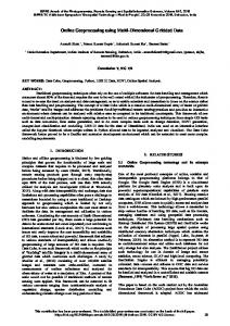
ISPRS Annals of the Photogrammetry, Remote Sensing and Spatial Information Sciences, Volume II-3/W2, 2013 ISA13 - The ISPRS Workshop on Image Sequence Analysis 2013, 11 November 2013, Antalya, Turkey In the following sequences, points that are being successfully tracked are marked as green, while those that are occluded or mismatched are marked as red. This determination is made using a normalized cross-correlation template match of the current tracked feature compared to a weighted average of its appearance in previously tracked frames. Sequence 1 - In Figure 2, tracking results are shown for a simple dataset taken in a parking lot. In this sequence, the photographer is walking, adding a significant amount of shaky movement and motion blur in the scene. As a result, KLT struggles to maintain quality correspondences. The proposed method struggles in some areas due to the jerky motion, but still provides vastly superior results to those from the appearance-based approach. Even when large displacements persist between two frames, the derived geometry is able to retain the feature tracking successfully. Sequence 2 – In Figure 3, tracking results are shown for an electronically captured aerial dataset of a model city. In this sequence, the aircraft is revolving around the scene with a relatively low frame-rate, thus causing feature perspectives to rapidly change. The proposed tracker provides acceptable tracking results thanks to its geometric constraints. The KLT tracker does not perform quite as well on this dataset. Almost immediately, KLT begins mismatching points due to the drastic appearance shifts. Points in the middle of the scene, where perspective doesn’t change as rapidly, are successfully tracked by both methods. Around the edges of the sequence, however, large appearance changes cause KLT to fail while the proposed method continues to track the features. Mean Error (pixels)

KLT Proposed (KLT Init.) Proposed (GT Init.)

0.9271 0.8490 0.2270

to multiple anomalies that have plagued tracking algorithms since their inception.

5. REFERENCES S.S. Beauchemin and J. L. Barron, 1995. The computation of optical flow. ACM Computing Surveys Vol. 27 No. 3 pp. 433-66. David J. Fleet and Yair Weiss, 2006. Optical flow estimation. Handbook of Mathematical Models in Computer Vision. By Nikos Paragios, Yunmei Chen, and Olivier Faugeras. New York: Springer. C. Hue, J.L. Cadre, and P. Prez, 2002. Sequential monte carlo methods for multiple target tracking and data fusion. IEEE Trans. on Signal Processing. Vol. 50. No. 2, pp 309–325 Bruce D. Lucas and Takeo Kanade, 1981. An iterative image registration technique with an application to stereo vision. Image Understanding Workshop. pp. 121-30. H. Schweitzer, J.W. Bell, and F. Wu, 2002. Very fast template matching. European Conf. on Computer Vision, pp. 358–372. K. Shafique and M. Shah. 2003. A non-iterative greedy algorithm for multi-frame point correspondence.” IEEE Int. Conf. on Computer Vision, pp. 110–115. Linda G. Shapiro and George C. Stockman, 2001. Computer Vision. Upper Saddle River, NJ. Prentice Hall. Carlo Tomasi and Takeo Kanade, 1991. Detection and tracking of point features. International Journal of Computer Vision. Carlo Tomasi and Takeo Kanade. 1992. Shape and motion from image streams under orthography: a factorization method. International Journal of Computer Vision. Vol. 9, No. 2, pp. 137-54.

Std. Dev. Error (pixels)

1.1125 1.2280 0.1138

Alper Yilmaz, Omar Javed, and Mubarak Shah, 2006. Object tracking – a survey. ACM Computing Surveys Vol. 38, No. 4

Table 1. Quantitative accuracy comparison between two implementations of the proposed method and the well-known KLT method shows a tracking improvement on the synthetic dataset.

Sequence 3 – In Figure 4, tracking results are shown for a dataset purposely captured to show the proposed algorithm’s resistance to point occlusion. In this sequence, a pedestrian walks through the scene from right to left, causing all features to become occluded and then reappear. KLT has no means of retaining or recovering the occluded points; once they become occluded they are lost forever. Meanwhile, the proposed method recognizes the points are occluded based on template matching comparisons and automatically begins tracking based on the object’s known shape. While points are occluded they remain correctly tracked by using the projection information provided by the non-occluded points. Once they reappear in the scene, the algorithm recognizes the change and automatically begins tracking them as before. 4. CONCLUSIONS This paper introduces a new method for geometrically constraining existing point tracking methods to promote continued improvement on tracking quality. This geometric component collaborates seamlessly with the existing appearance component to provide a checks-and-balances system to tracking features in a scene. As a result, when one component fails, the other is there to ensure quality is not lost. Our experiments have shown that the introduced component outperforms the existing KLT method in real-life datasets as well as provides robustness

This contribution has been peer-reviewed. The double-blind peer-review was conducted on the basis of the full paper.

29

ISPRS Annals of the Photogrammetry, Remote Sensing and Spatial Information Sciences, Volume II-3/W2, 2013 ISA13 - The ISPRS Workshop on Image Sequence Analysis 2013, 11 November 2013, Antalya, Turkey

Figure 2. Tracking comparison between the proposed method (top) and KLT (bottom) shows a significant tracking improvement when geometric constraints are added to the system. While KLT struggles with motion blur and large displacements, the object shape in the proposed method retains tracking accuracy.

Figure 3. Tracking comparison between the proposed method (top) and KLT (bottom) shows a significant tracking improvement on this aerial dataset, especially along image borders where the camera perspective drastically skews feature appearance.

Figure 4. Tracking comparison between the proposed method (top) and KLT (bottom) shows a significant tracking improvement when occlusion is present.

This contribution has been peer-reviewed. The double-blind peer-review was conducted on the basis of the full paper.

30