IEEE GEOSCIENCE & REMOTE SENSING LETTERS
1
Robust ground peak extraction with range error estimation using full-waveform LiDAR Andr´e Jalobeanu and Gil Gonc¸alves
Abstract—Topographic mapping is one of the main applications of airborne LiDAR. Waveform digitization and processing allow for both an improved accuracy and a higher ground detection rate compared to discrete return systems. Nevertheless, the quality of the ground peak estimation, based on last return extraction, strongly depends on the algorithm used. Bestperforming methods are too computationally intensive to be used on large datasets. We used Bayesian inference to develop a new ground extraction method whose most original feature is predictive uncertainty computation. It is also fast, and robust to ringing and peak overlaps. Obtaining consistent ranging uncertainties is essential for determining the spatial distribution of error on the final product, point cloud or DEM. The robustness is achieved by a partial deconvolution followed by a Bayesian Gaussian function regression on optimally truncated data, which helps reduce the impact of overlapping peaks from low vegetation. Results from real data are presented, and the gain with respect to classical Gaussian peak fitting is assessed and illustrated.
I. I NTRODUCTION Topographic mapping using laser ranging is rapidly expanding, as it provides dense and accurate measurements at a competitive cost [2]. Recently, full-waveform data have become more easily available, as most LiDAR systems now offer waveform digitization capabilities. This offers substantial benefits over discrete return systems, provided that one is able to process the large volumes of recorded data [3], [4]. In this paper, we focus on topographic mapping in vegetated areas. The main problem consists of recovering the last peak within each waveform. This peak corresponds to the ground return, when the vegetation allows for enough penetration and when there are no buildings. Here, we do not consider the filtering that might be necessary when the ground is not reached. In this paper we address a signal processing problem, treating each waveform independently. We mainly aim at the recovery of the peak position (or timing) and its error, and provide amplitude and other attributes as by-products. Range computation and georeferencing are out of the scope of this paper, despite being necessary to derive results from real data (see Sec. V). We adopt a probabilistic approach [5] to peak detection and extraction, based on Bayesian inference [6]. In this framework, all parameters are random variables, and we are interested in inferring their probability density function (pdf). Models are defined using available knowledge, which helps greatly to The data acquisition and part of the present study were funded by the Foundation for Science and Technology (FCT) of Portugal, in the framework of the AutoProbaDTM research project [1], with co-funding by FEDER (PTDC/EIA-CCO/102669/2008, FCOMP-01-0124-FEDER-010039). A. Jalobeanu is with University of Texas at Austin and works at NPS Monterey, CA, USA; contact:
[email protected] G. Gonc¸alves is with University of Coimbra and INESCC, Portugal
simplify the procedure; e.g. the peak shape and the noise properties are either known or derived from calibration. Inference consists of automatically estimating the pdf of the quantity of interest, which can be summarized by an optimal value and an uncertainty. We have reduced user-supplied parameters to a minimum, as only the false alarm rate has to be chosen. The predictive error estimate enables us to objectively quantify the expected quality of the result from available data only, and allows for rigorous error propagation through to the end product. It is therefore a product of remarkable added-value, not provided by existing methods. The algorithm presented here is original, as it provides an error estimate while existing methods do not. Also, the detection technique uses as much data samples as possible, unlike second-derivative zero-crossing or leading edge thresholding [2], whether applied to the original signal or a spline or wavelet representation. Differences with other methods that make use of all the data are explained in Sec. II through IV. The proposed method consists of two steps, and is presented as follows: step 1, seeking to reduce system response artifacts, is detailed in Sec. II. We introduce a robust estimator based on data truncation in Sec. III, then give the details of step 2, the automatic Bayesian detection and inference for a single Gaussian peak, in Sec. IV. To support our claims and illustrate our contributions, we show results from real data in Sec. V. II. PARTIAL DECONVOLUTION The first step of the processing is a partial deconvolution. It is partial as it does not try to fully invert the effect of the system impulse response (IR). Instead, it is designed to only correct the ringing artifacts and remove the trailing edge, thus aiming at a more convenient Gaussian IR. This reduces the number of false alarms (typically underground returns) by avoiding false detections arising from these artifacts [7]. Indeed, in this step we aim at the recovery of a waveform as a back-scatter cross-section convolved with a simple Gaussian IR function, so that the data can be further processed by assuming that the peak of interest is a Gaussian function. An alternative approach would have been to model this peak as the system IR in the Bayesian inference procedure (see Sec. III) but it would have resulted in an increased complexity, compared to the two-step approach we adopted. Complete deconvolution [8], [9], aiming at the correction of the full effect of the IR, is generally motivated by the determination of a physical target cross-section. However, it is inappropriate in our case, as we are only interested in the last scatterer. This is an ill-posed inverse problem as explained in
2
IEEE GEOSCIENCE & REMOTE SENSING LETTERS
i
The peaks have discrete locations to simplify the problem. This way, the waveform deconvolution is done with a discrete kernel H, which is sparse, and whose non-zero coefficients are i at time ⌧i (see Fig. 1 right). This only inverts the effect of the mixture, and not that of the Gaussian G; nothing is done if only the first coefficient is non-zero. The sparsity of the kernel and relative small amplitude of secondary coefficients enable us to implement a fast, efficient deconvolution that is well-posed, therefore it does not need any regularization or tuning of the related parameters. The deconvolution amounts to the inversion of the linear equation y = H ?Y where y is the recorded data and Y the deconvolved waveform. For the seven coefficients i we only need two iterations using a conjugate gradient algorithm, so the overhead introduced by this step is negligible. However, the benefits are considerable, especially for high-amplitude peaks where the ringing is significant. In this study, the IR was calibrated from the raw data acquired with a Riegl LMS-Q680i airborne scanner [12], assuming that it is not amplitude-dependent (linear system). This calibration needs to be done regularly for each sensor. The received peaks having the highest amplitudes were selected in order to maximize the quality. No outgoing pulses were used as they are not digitized by the same channel. In this study we only considered the low-power channel [13], as high power returns were extremely rare due to the flight parameters (see Sec. V). The calibration was done for amplitudes at which it matters most, so any amplitude-dependence would only affect weak returns, for which deconvolution is not as crucial. The faintest returns are not corrected, when secondary peak amplitude is less than one quantization unit. Fig. 1 (left)
shows 100 waveforms of amplitude above 70, normalized to a maximum amplitude of one and stacked, before and after deconvolution: notice both ringing and trailing edge reduction. We have w = 4 with 1 ns sampling interval. 0 1
coefficients κi
τi κi
digital number / raw amplitude
[8], especially since the waveform sampling rate exceeds twice the Nyquist rate [10] in most scanners. Therefore it requires strong prior knowledge, effective regularization and a good model in order to avoid reconstruction artifacts (even more ringing and noise amplification). Solving it is computationally intensive and the solution is sensitive to noise, parameter values and convergence issues as reported in [9]. There is a severe information loss due to the band-limiting (or lowpass) effect of the IR affecting the highest frequencies [10], which can only be addressed with proper prior modeling and complex optimization methods. Such effort would be mostly wasted as we are only interested in the last peak. In [11] the regularization issue is circumvented thanks to redundancy, as the parameter spacing is twice the sampling interval and the bandlimiting effects of the IR is taken into account through the use of B-Splines; the technique is reasonably fast. Due to this spacing, the technique has a behavior similar to the partial deconvolution that we advocate. Nevertheless, our method is simpler to implement and has a lower computational complexity. We model the system IR denoted by h as a mixture of Gaussians denoted by Gw , of full width at half maximum w (as an approximation, we assume that the secondary peaks have the same width as the main peak; it is justified by their small relative amplitude, less than 5% of the main). X 2 2 h(t) = i Gw (t ⌧i ) with Gw (t) = e (4 log 2) t /w (1)
time (ns)
times τi (ns)
5
11
16
20
24
28
0.030 0.045 0.015 0.012 0.008 0.005
Fig. 1. Left: received high amplitude waveforms (Riegl LMS-Q680i low channel), centered and normalized; original (red) and after partial deconvolution (blue). Right: discrete convolution kernel H, calibrated from the data.
III. ROBUST ESTIMATION OF PEAK TIMING We only use the deconvolved waveform data Y from now on. We choose to use a single Gaussian peak to model Y , rather than a mixture. To derive a method that is robust to overlaps (when the left side of the ground peak is contaminated by nearby peaks from low vegetation, animals or objects, received just before the ground return), it seems natural to perform a Gaussian decomposition, using techniques from [14] or [15], then keep the last peak. Unfortunately, not only are these methods complex, as they rely on nonlinear optimization, they are also unstable and lack robustness. Indeed, the number of estimated peaks, their width and location are sensitive to noise, and the decomposition suffers from inherent nonuniqueness even for high quality signals. Constraints are introduced to tackle these issues. Fully Bayesian techniques provide a mathematically optimal treatment, allowing for Bayesian model selection [16] and determination of the number of peaks. Usually a stochastic optimization is required, as in [17], which is time consuming, and significantly slower than the deterministic non-linear fitting methods mentioned above. Bayesian inference usually requires rigorous modeling of all the data; one cannot specify only the last peak (of interest) without explicitly modeling the left side of the signal, e.g. via a Gaussian mixture, with the issues mentioned above. To avoid that, we chose to truncate the data Y , assuming a single peak within a discrete time interval [tl , n 1] where n is the data size, regardless of the samples before tl . Although this approach may not be strictly Bayesian, it limits the number of unknown parameters and allows for deterministic and fast processing. We propose to extend the three-point estimator, consisting of using the last discrete maximum and its two neighbors; for Gaussian peaks, quadratic interpolation of the log of the data (after background subtraction) provides location, width and amplitude, as shown in [18]. The advantage is that it is insensitive to all the samples before the three used ones, which makes it more robust to overlapping peaks than a full Gaussian fit, however it yields lower performance for clean peaks as it only uses a small fraction of the data. We use all the following samples as well, and apply Bayesian inference to the truncated dataset defined by Dl ⌘ {Yt }tl t 34 w and comparable amplitudes, wich includes many realistic scenarios. A
and for convenience µ is subtracted from the raw waveforms before processing. Thanks to the independence assumption, the likelihood writes as a product over samples indexed by t: 2 Y 2 P (Dl | t0 , A, w) / e Yt A Gw (t t0 ) /2 n (4) tl t T . It is also implemented as a discrete search, but in the log space as log P is nearly quadratic near the optimum. We use a step 0.5 (half the sampling interval). Finally a Newton refinement iteration (using numerical derivatives) allows us to achieve a subsample accuracy. The algorithm consists of an outer loop defined by procedure 1, and two inner loops with tl equal to th and tf for the truncated and full estimators, respectively. The value of tf should be th wmax , allowing us to ignore peaks separated from the last by at least the maximum width. Regarding the definition of tf , just setting tf = 0 is equivalent, although slightly slower as more data samples might be used. The search within procedure 1 continues until a valid optimum has been found by procedure 2. All constraints, including minimum peak width and maximum timing uncertainty (see
4
IEEE GEOSCIENCE & REMOTE SENSING LETTERS
Sec. IV-C), are far more stringent than the condition on the discrete search. The optimal estimator is selected automatically (see Sec. IV-E). False alarm rates for procedure 1 are fixed by the user through the value of T and can be determined using simulations. For white noise for instance, T = 2.5 n ensures a rate lower than 10 6 (see Sec. IV-D for more practical details). Faint return recovery is possible if neighborhood information is available: we used a scanline-based predictive filtering to get the expected peak timing for ground returns hidden under vegetation. Relaxing the search conditions while using this prior knowledge allowed us to recover half of the waveforms otherwise rejected by the filtering algorithm [1]. C. Uncertainty estimation and proxies The predictive uncertainty is given by the width of the posterior marginal pdf of the parameters of interest [16], and can be approximated by assuming a Gaussian posterior and estimating its standard deviation. This is done by calculating second derivatives around the optimum tˆ0 . The sought uncertainty is denoted by t : ⇣h @ 2 i ⌘ 1/2 log P (t0 | Dl ) (7) t = @t0 t0 =tˆ0 Due to the limitations of the assumed noise model, and to the randomness of the data that impacts the computation of derivatives, we choose to define proxy functions f in order to provide a simpler, and especially more robust, uncertainty estimation procedure. In practice t should only depend on the noise properties, the peak shape, and the type of estimator denoted by m, with m 2 {h, f }. When noise correlation is significant, this allows us to update the uncertainty without changing the estimator. The following proxy (8) is derived from simulations with various peak shapes and noise levels. ⇢ is the correlation coefficient, K and p are constants, calibrated using simulations. A is the raw amplitude, A 2 [0, 255]. n
wpm,⇢ (8) A For instance, for a low amplitude A = 5, with n = 1, ⇢ = 0.75 and 1.5 widening (w = 6) and the truncated estimator, we have t = 1 ns, or 15 cm error (±30 cm accuracy [2]). t
' fm,⇢ (A,
n , w)
= Km,⇢
p / 1 + "Yt and the constant " is small enough so that n ⇠ is the same order of magnitude over the admissible amplitude range. The relative increase in uncertainty is significant only for high amplitudes, but then t becomes very low from (8) – so low that other factors have to be taken into account, such as GPS errors (0.5 cm at best), therefore the contribution of the ranging error, and the value of ", become irrelevant. n
E. Choosing the optimal estimator to achieve robustness We seek to minimize both bias and variance by choosing the best estimator [5] depending on the data, so a full peak model can be used when no overlap is detected. We propose to use a chi-squared test [5], checking the statistical significance of the residual error. The data interval is provided by the full estimator. The peak model is obtained from the truncated data Dl (so that the left side of the peak will exhibit residuals larger than n in case of overlap). Noise correlation is accounted for by correcting the residual threshold. We also test the significance of the bias reduction, so the full estimator is selected when the difference between timing estimators falls within a predefined confidence interval (e.g. 95%) given by the predictive uncertainty (7). Finally, the proposed approach is tested using simulations in the same configuration as in Fig. 2 but with noise added, and two ground peak amplitudes. Fig. 3 illustrates these tests. Predictive (A) and actual (B) uncertainties are compared, showing a good agreement except in a narrow region where t ' w, and peaks have comparable amplitude (uncertainty underestimation by a factor 2 at worst). Both timing accuracy and uncertainty prediction improve with higher peak amplitudes, as the SNR increases. As expected, full peak estimates tend to be selected when there is little overlap. This also occurs in narrow separation cases, as peaks become indistinguishable. The robustness of the overall approach clearly outperforms that of classical Gaussian fitting, as shown in Fig. 3 (we did not include bias and widening plots as they are very similar to Fig. 2). We also provide a comparison online [1] from real data, as a separate layer named ”range bias”, defined by the range difference between the two methods. A
D. Departure from simple noise assumptions
B
contaminant/main peak amplitude ratio
We modeled neither noise correlation, nor its dependence upon amplitude. In practice, we found a high correlation ⇢=0.75 on the Riegl LMS-Q680i. This is due to the hardware digitizer and not to our deconvolution step. No significant changes were observed before and after this step. As a consequence, the actual uncertainties might be higher than the ones predicted using the white noise assumption. Simulations confirmed this fact. Updating the estimators to take that into account is possible but the added complexity is not justified by the gain in variance or robustness, hence the use of the proxy (8). To achieve a false alarm rate of 10 6 we set T = 4 n . The dependence of n on Yt , due to the photon noise component, is not obvious from direct observations or fit residuals. The instrument is operated in a high photon-count regime and this effect might be negligible. If not, we have
peak separation (samples)
main peak amplitude = 10
main peak amplitude = 50
Fig. 3. Quality assessment of the robust estimator uncertainty t in various configurations of peak overlap (same as in Fig. 2), 500 simulated waveforms per point, white Gaussian noise of variance 1. A: computed mean predictive time uncertainty; B: empirical time uncertainty.
5
V. R ESULTS The AutoProbaDTM project focused on the development of new data processing methods for automated and largescale topographic mapping, using large full-waveform LiDAR datasets (see website [1] for more information, final results and DEM distribution). The data used to test the new algorithms were acquired in June 2011, over a 200 km2 area chosen for its geomorphological interest, NW of Arraiolos (Portugal). A Riegl LMS-Q680i was flown at 1500 m AGL. A return density between 3 and 4 pts/m2 was obtained and 5.60⇥108 waveforms were recorded. The processing required 3.5 hours (4 threads, Intel Core i7 2.67 MHz) including file decoding, emitted pulse timing and sorting, outlier rejection, geometric computations and gridding. Half of this time was spent on the original procedures required by our new method, indicating that it is only two times slower than single Gaussian fitting. Finally 5.30⇥108 points were obtained – with elevation uncertainty, intensity and pulse width attributes. The results were gridded at 1 m GSD and 1 km2 GeoTIFF tiles were distributed. Fig. 4 shows six waveforms after deconvolution, the inferred ground peaks using both full and truncated estimators, and the selected robust result, which is satisfactory even at low amplitudes. Correlated noise is visible as small oscillations or peaks after the ground peaks. Inspection of the final results showed no evidence of false alarms underground. However, there are significant false detections above ground that are mostly due to vegetation opacity, and for which independent waveform processing fails, thus requiring a filtering procedure. A preliminary consistency check of the uncertainties was done on water bodies, assumed flat. Therefore over a short interval the extracted points should lie on a straight line even without georeferencing. We found that the error bars are consistent with line fitting: see Fig. 5 for an illustration. Deconvolved wave Robust last peak extraction Truncated Gaussian peak estimator
digital number (multiples of 20 added for convenience)
Full Gaussian peak estimator
time (ns)
range
1m
Fig. 4. Examples of ground peak extraction from real waveforms. Full and truncated estimators (thin lines), and selected or robust estimator (thick line).
0.208 ms
time
Fig. 5. Range as a function of time, collected over a water body during a short interval. Extracted points with error bars (red) and line fitting (blue).
VI. C ONCLUSION The main contribution of this work is to provide the ability of extracting point clouds (and also derived products such as DEM) with spatially variable predictive uncertainties or error maps. As opposed to validation procedures [2] which only compute global error statistics, we provide one error estimate with each point. These spatial errors are required for the rigorous, quantitative analysis of topographic data [19], and are crucial for applications such as hydrology or change detection. This was made possible by applying Bayesian inference to waveform data processing, thus deriving a novel ground peak estimation algorithm that is both fast and robust to noise, sensor artifacts and overlaps from low vegetation. R EFERENCES [1] (2013). [Online]. Available: http://sites.google.com/site/autoprobadtm [2] J. Shan and C. K. Toth, Topographic laser ranging and scanning: principles and processing. CRC Press, 2008. [3] A. Chauve, C. Mallet, F. Bretar, S. Durrieu, M. P. Deseilligny, and W. Puech, “Processing full-waveform lidar data: modelling raw signals,” in ISPRS Archives, vol. XXXVI-3/W52, Espoo, Finland, 2007, pp. 102– 107. [4] C. Mallet and F. Bretar, “Full-waveform topographic lidar: State-of-theart,” ISPRS Journal of Photogrammetry and Remote Sensing, vol. 64, no. 1, pp. 1–16, 2009. [5] E. T. Jaynes, Probability Theory: The Logic of Science. Cambridge University Press, Jun. 2003. [6] J. M. Bernardo and A. F. M. Smith, Bayesian Theory, 1st ed. John Wiley & Sons, 1994. [7] A. Roncat, W. Wagner, T. Melzer, and A. Ullrich, “Echo detection and localization in full-waveform airborne laser scanner data using the averaged square difference function estimator,” The Photogrammetric Journal of Finland, vol. 21, no. 1, pp. 62–75, 2008. [8] Y. Wang, J. Zhang, A. Roncat, C. K¨unzer, and W. Wagner, “Regularizing method for the determination of the backscatter cross section in lidar data,” J. Opt. Soc. Am. A, vol. 26, no. 5, pp. 1071–1079, May 2009. [9] C. E. Parrish, I. Jeong, R. D. Nowak, and R. B. Smith, “Empirical comparison of full-waveform lidar algorithms: Range extraction and discrimination performance,” Photogrammetric Engineering and Remote Sensing, vol. 77, no. 8, pp. 824–838, 2011. [10] A. K. Jain, Fundamentals of digital image processing. Prentice-Hall Englewood Cliffs, 1989, vol. 3. [11] A. Roncat, G. Bergauer, and N. Pfeifer, “B-spline deconvolution for differential target cross-section determination in full-waveform laser scanning data,” ISPRS Journal of Photogrammetry and Remote Sensing, vol. 66, no. 4, pp. 418–428, 2011. [12] (2013). [Online]. Available: http://products.rieglusa.com/category/ airborne-scanners [13] A. Jalobeanu and G. R. Gonc¸alves, “The full-waveform LiDAR Riegl LMS-Q680i: from reverse engineering to sensor modeling,” in American Society of Photogrammetry and Remote Sensing Annual Conference, Sacramento, CA, USA, Mar 2012. [14] M. A. Hofton, J. B. Minster, and J. B. Blair, “Decomposition of laser altimeter waveforms,” Geoscience and Remote Sensing, IEEE Transactions on, vol. 38, no. 4, pp. 1989–1996, 2000. [15] W. Wagner, A. Ullrich, V. Ducic, T. Melzer, and N. Studnicka, “Gaussian decomposition and calibration of a novel small-footprint full-waveform digitising airborne laser scanner,” ISPRS Journal of Photogrammetry and Remote Sensing, vol. 60, no. 2, pp. 100–112, 2006. [16] D. S. Sivia, Data Analysis: A Bayesian Tutorial. Oxford University Press, 1996. [17] C. Mallet, F. Lafarge, M. Roux, U. Soergel, F. Bretar, and C. Heipke, “A marked point process for modeling lidar waveforms,” Image Processing, IEEE Transactions on, vol. 19, no. 12, pp. 3204–3221, 2010. [18] J. Li, J. D. Valentine, and A. E. Rana, “The modified three point gaussian method for determining gaussian peak parameters,” Nuclear Instruments and Methods in Physics Research Section A, vol. 422, no. 1, pp. 438– 443, 1999. [19] S. P. Wechsler and C. N. Kroll, “Quantifying dem uncertainty and its effect on topographic parameters,” Photogrammetric Engineering and Remote Sensing, vol. 72, no. 9, pp. 1081–1090, 2006.