Robust Inference for Generalized Linear Models Eva Cantoni and Elvezio Ronchetti
Department of Econometrics University of Geneva CH - 1211 Geneva 4, Switzerland May 1999 Revised January 2001 Abstract By starting from a natural class of robust estimators for generalized linear models based on the notion of quasi-likelihood, we define robust deviances that can be used for stepwise model selection as in the classical framework. We derive the asymptotic distribution of tests based on robust deviances and we investigate the stability of their asymptotic level under contamination. The binomial and Poisson models are treated in detail. Two applications to real data and a sensitivity analysis show that the inference obtained by means of the new techniques is more reliable than that obtained by classical estimation and testing procedures.
1
Introduction
Generalized linear models (McCullagh and Nelder, 1989) are a powerful and popular technique for modeling a large variety of data. In particular, generalized linear models allow to model the relationship between the predictors and a function of the mean of the response for continuous and discrete response variables. The response variables Yi , for i = 1, . . . , n are supposed to come from a distribution belonging to the exponential family, such that E[Yi ] = µi and V[Yi ] = V (µi ) for i = 1, . . . , n and ηi = g(µi ) = xTi β, i = 1, . . . , n,
(1)
where β ∈ IRp is the vector of parameters, xi ∈ IRp , and g(.) is the link function. The non-robustness of the maximum likelihood estimator for β has been studied extensively in the literature: cf. for instance the early work of Pregibon (1982) on logistic regression, Stefanski, Carroll, and Ruppert (1986), K¨ unsch, Stefanski, and Carroll (1989), Morgenthaler (1992), and Ruckstuhl and Welsh (1999). In more recent work, Preisser and Qaqish (1999) consider a class of robust estimators in the general framework of generalized estimating equations. The quasi-likelihood estimator of the parameter of model (1) (see Wedderburn, 1974, McCullagh and Nelder, 1989, and Heyde, 1997) shares the same non-robustness properties. This estimator is the solution of the system of estimating equations n n X X (yi − µi ) 0 ∂ Q(yi , µi ) = µi = 0, ∂β V (µ ) i i=1 i=1
where µ0i =
∂ µ, ∂β i
(2)
and Q(yi , µi ) is the quasi-likelihood function. The solution of (2) is
an M-estimator (see Huber, 1981, and Hampel, Ronchetti, Rousseeuw, and Stahel, ˜ i , µi ) = 1986) defined by the score function ψ(y
(yi −µi ) 0 µ. V (µi ) i
Its influence function
(Hampel, 1974 and Hampel et al., 1986) is proportional to ψ˜ and is unbounded. 1
Therefore, large deviations of the response from its mean or outlying points in the explanatory variables xi can have a large influence on the estimator. Thus, the quasi-likelihood estimator – as well as the maximum likelihood estimator – is not robust. Several robust alternatives have been proposed in the literature; see the references given above. However, in spite of the fair amount of existing literature, robust inference for generalized linear models seems to be very limited. Moreover, only the logistic regression situation is usually considered in detail, and the problem of developing robust alternatives to classical tests is not addressed globally for the whole class of generalized linear models. In this paper we propose a robust approach to inference based on robust deviances which are natural generalizations of quasi-likelihood functions. Our robust deviances are based on the same class of robust estimators as that proposed by Preisser and Qaqish (1999) in the more general setup of generalized estimating equations. Although these estimators are not optimally robust, they form a class of M-estimators easy to deal with, and which admits handy inference not only for logistic regression but for the whole class of generalized linear models. One could argue that two alternative approaches could be considered. A first possibility would be to view variable selection as a parametric hypothesis and to use Wald, score or likelihood ratio tests for which robust versions are available; see e.g. Heritier and Ronchetti (1994) and Markatou and He (1994). While this would in principle be feasible, Wald and score tests do not seem to be used much in the classical analysis of generalized linear models. Moreover, robust likelihood ratio tests cannot be proposed in this case, because the optimal robust score function does not admit an analytic primitive function and numerical integration in the space
2
of parameters for computing such a primitive is generally unfeasible. A second approach would be to rely on the robust model selection based on Akaike Criterion, Mallows’ Cp or similar techniques; see e.g. Ronchetti and Staudte (1994), Sommer and Huggins (1996) and Ronchetti (1997) for a review. This approach has the advantage to perform a full model search. However, when the number of variables is moderate to large such a full search is impossible and a stepwise selection is the only feasible alternative. For these reasons and in view of the importance of the notion of deviance for model building in generalized linear models, we propose robust deviances based on generalizations of quasi-likelihood functions. The general structure of the classical approach by quasi-likelihood is preserved, which offers the advantage of having robust tools playing the same role as deviances, anova tables, stepwise procedures, and so on. The paper is organized as follows. In the next section we discuss robust estimators of a generalized linear model based on quasi-likelihood. As an illustration, we focus in particular on the estimation of binomial and Poisson models. In Section 3, we discuss inference and propose a family of test statistics for model selection. We derive their asymptotic distribution through the development of an asymptotically equivalent quadratic form and we study their robustness properties through the influence function. Section 4 presents some computational aspects and Section 5 gives two applications. Finally, in Section 6 we discuss some potential research directions.
3
2
Robust Estimation Based on Quasi-likelihood
2.1
General Definition
We consider a general class of M-estimators of Mallows’s type, where the influence of deviations on y and on x are bounded separately. The estimator is the solution of the estimating equations:
n X
ψ(yi , µi ) = 0,
(3)
i=1
where ψ(y, µ) = ν(y, µ)w(x)µ0 − a(β), a(β) =
1 n
Pn
i=1
E[ν(yi , µi )]w(xi )µ0i with the
expectation taken with respect to the conditional distribution of y|x, ν(·, ·), w(x)
are weight functions defined below, and µi = µi (β) = g −1 (xTi β). The constant
a(β) ensures the Fisher consistency of the estimator. The estimating equation (3) for generalized linear models is a special case of equation (1) p. 575 for generalized estimating equations in Preisser and Qaqish (1999), where our function ν(y, µ)w(x) is (in their notation) V −1 (µ)w(x, y, β)(y − µ) and a(β) = µ0 V −1 (µ) c.
Let y = (y1 , . . . , yn )T and µ = (µ1 , . . . , µn )T . The estimating equation (3)
corresponds to the minimization of the quantity QM (y, µ) =
n X
QM (yi , µi ),
(4)
i=1
with respect to β, where the functions QM (yi , µi ) can be written as Z µi n Z ¤ 1 X µj £ QM (yi , µi ) = ν(yi , t)w(xi )dt − E ν(yj , t)w(xj ) dt, n j=1 t˜ s˜
(5)
with s˜ such that ν(yi , s˜) = 0, and t˜ such that E[ν(yi , t˜)] = 0. Note that differences of deviances, as the test statistic (8), are independent of s˜ and t˜. The structure of (3) is suggested by the classical quasi-likelihood equations. The estimator defined by equation (3) is an M-estimator characterized by the score func4
tion ψ(yi , µi ) = ν(yi , µi )w(xi )µ0i − a(β). Its influence function is then IF(y; ψ, F ) =
∂ M (ψ, F )−1 ψ(y, µ), where M (ψ, F ) = −E[ ∂β ψ(y, µ)]; cf. Hampel et al. (1986).
Moreover, the estimator has an asymptotic normal distribution with asymptotic variance Ω = M (ψ, F )−1 Q(ψ, F )M (ψ, F )−1 , where Q(ψ, F ) = E[ψ(y, µ)ψ(y, µ)T ]. It is then clear that the choice of a bounded function ψ ensures robustness by putting a bound on the influence function. Therefore, a bounded function ν(y, µ) is introduced to control deviations in the y-space, and leverage points are down-weighted by the weights w(x). Simple choices for ν(·, ·) and w(·) suggested by robust estimators √ in linear models are ν(yi , µi ) = ψc (ri ) V 1/21(µi ) (see (6) below) and w(xi ) = 1 − hi , where hi is the i-th diagonal element of the hat matrix H = X(X T X)−1 X T . More
sophisticated choices for w(·) are available (see Staudte and Sheather, 1990, p. 258, for a discussion in linear regression or Carroll and Welsh, 1988). Weights defined on H do not have high breakdown properties, and from this point of view, other choices of w(xi ) are more suitable. For example, w(xi ) can be chosen as the inverse of the Mahalanobis distance defined through a high breakdown estimate of the center and of the covariance matrix of the xi (see, for example, the minimum volume ellipsoid estimator or the minimum covariance determinant estimator in Rousseeuw and Leroy, 1987, p. 258 ff.). Finally notice that the choice of ν(yi , µi ) =
yi −µi V (µi )
and
w(xi ) = 1 for all i, recovers the classical quasi-likelihood estimator, so that for a judicious choice of ν(yi , µi ) and of the weights w(xi ), the function QM (y, µ) can be seen as the robust counterpart of the classical quasi-likelihood function. The form of this estimator is attractive because the estimating equation (3) corresponds to the minimization of (4) and this leads to a natural definition of robust deviance; see Section 3.1.
5
2.2
Robust Estimation for Binomial and Poisson Models
We consider here the particular case of (3), defined by ν(yi , µi ) = ψc (ri ) V 1/21(µi ) , where ri =
yi −µi V 1/2 (µi )
are the Pearson residuals and ψc is the Huber function defined
by
r | r |≤ c, ψc (r) = c sign(r) | r |> c.
(6)
We call the estimator defined in this way, the Mallows quasi-likelihood estimator. It solves the set of estimating equations n h X
ψc (ri )w(xi )
i=1
where a(β) =
1 n
Pn
i=1
i 1 0 µ − a(β) = 0, V 1/2 (µi ) i
(7)
E[ψc (ri )]w(xi ) V 1/21(µi ) µ0i . Using the same notation as in the
linear regression case, when w(xi ) = 1 we call this estimator Huber quasi-likelihood estimator. The tuning constant c is typically chosen to ensure a given level of asymptotic efficiency. In Section 3.2 we propose an alternative procedure for the choice of the tuning constant. a(β) is a correction term to ensure Fisher consistency; see Hampel et al. (1986) for general parametric models and He and Simpson (1993), Section 4.1, for power series distributions. Note that a(β) can be computed explicitly for binomial and Poisson models and does not require numerical integration; cf. Appendix A. The matrices M (ψ c , F ) and Q(ψ c , F ) can also be easily computed for the Mallows quasi-likelihood estimator: Q(ψ c , F ) =
1 T X AX − a(β)a(β)T , n
1 where A is a diagonal matrix with elements ai = E[ψc (ri )2 ]w2 (xi ) V (µ ( ∂µi )2 , and i ) ∂ηi
M (ψ c , F ) = 6
1 T X BX, n
i 2 where B is a diagonal matrix with elements bi = E[ψc (ri ) ∂µ∂ i log h(yi |xi , µi )] V 1/21(µi ) w(xi )( ∂µ ), ∂ηi
and h(·) is the conditional density or probability of yi |xi . We refer to Appendix B for further details and for the computation of these matrices for binomial and Poisson models.
3
Robust Inference
3.1
Model Selection Based on Robust Deviances
The function QM (y, µ) defined in (4) and (5) allows to develop robust tools for inference and model selection based on robust quasi-deviances. Denote by a = (aT(1) , aT(2) )T the partition of a vector a into (p − q) and q components and the corresponding partition of a matrix A by A11 A12 , A= A21 A22 where A11 ∈ IR(p−q)×(p−q) , A12 ∈ IR(p−q)×q , A21 ∈ IRq×(p−q) and A22 ∈ IRq×q . To evaluate the adequacy of a model, we define a robust goodness-of-fit measure — called robust quasi-deviance — based on the notion of robust quasi-likelihood function, i.e. DQM (y, µ) = −2QM (y, µ) = −2
n X
QM (yi , µi ),
i=1
where QM is defined by (4) and (5). DQM (y, µ) describes the quality of a fit and will be used to define a statistic for model selection. Let us consider the model Mp , with p parameters. Suppose that the corresponding set of parameters is β = (β1 , . . . , βp )T = (β T(1) , β T(2) )T . We are interested in testing the null hypothesis H0 : β (2) = 0. This is equivalent to 7
consider a nested model Mp−q ⊂ Mp with (p − q) parameters, and testing whether the sub-model Mp−q holds. We estimate the vector of parameters by solving (3) for the complete model, and ˆ of β. Under the null hypothesis, the same procedure yields we obtain an estimator β ˆ and µ˙ for the estimated linear predictors an estimator β˙ of (β (1) , 0). We write µ ˆ and β˙ respectively. Then, we define a robust measure associated to the estimate β of discrepancy between two nested models by h i ˙ − DQM (y, µ) ˆ ΛQM = DQM (y, µ) = 2
n hX i=1
QM (yi , µ ˆi ) −
n X i=1
i
QM (yi , µ˙ i ) ,
(8)
where the function QM (yi , µi ) is defined by (5). The statistic (8) is in fact a generalization of the quasi-deviance test for generalR µ −t ized linear models, which is recovered by taking QM (yi , µi ) = yi i yVi(t) dt. Moreover,
when the link function is the identity (linear regression), (8) becomes the τ -test statistic defined in Hampel et al. (1986), Chapter 7.
The same forms for the functions ν(yi , µi ) and w(xi ) as in the estimation problem can be considered here. In particular, a Mallows quasi-deviance statistic can be defined by taking ν(yi , µi ) = ψc (ri )/V 1/2 (µi ). The following Proposition establishes the asymptotic distribution of the test statistic (8). We assume the conditions for the existence, consistency, and asymptotic normality of M-estimators as given by (A.1)-(A.9) in Heritier and Ronchetti (1994), p. 902. These conditions have been studied by Huber (1967, 1981), Clarke (1986) and Bednarski (1993). Proposition 1 Under conditions (A.1)-(A.9) in Heritier and Ronchetti (1994), [C1], [C2] of Appendix C, and under H0 : β (2) = 0, the test statistic ΛQM defined 8
by (8) equals nLTn C(ψ, F )Ln + oP (1) = nRTn(2) M (ψ, F )22.1 Rn(2) + oP (1),
(9)
¡ ¢ ˜ + (ψ, F ), √nLn is normally distributed N 0, Q(ψ, F ) , where C(ψ, F ) = M −1 (ψ, F )−M √ M (ψ, F )22.1 = M (ψ, F )22 − M (ψ, F )T12 M (ψ, F )−1 nRn is nor11 M (ψ, F )12 , and ¡ ¢ mally distributed N 0, M −1 (ψ, F )Q(ψ, F )M −1 (ψ, F ) . Moreover, ΛQM is asymptotically distributed as q X
di Ni2 ,
i=1
where N1 , . . . , Nq are independent standard normal variables, d1 , . . . , dq are the q ¡ ¢ ˜ + (ψ, F ) , and M ˜ + (ψ, F ) positive eigenvalues of the matrix Q(ψ, F ) M −1 (ψ, F )− M
˜ + (ψ, F )11 = M (ψ, F )−1 ˜+ ˜+ is such that M 11 and M (ψ, F )12 = 0, M (ψ, F )21 = 0,
˜ + (ψ, F )22 = 0. M The proof is given in Appendix D. A similar result can be obtained for the distribution of ΛQM under contiguous alternatives β (2) = n−1/2 ∆. In such a case P 1/2 ΛQM is asymptotically distributed as qi=1 (di Ni + S T ∆)2 , where S is such that SS T = M22.1 and S T (M −1 (ψ, Fβ0 )Q(ψ, Fβ0 )M −1 (ψ, Fβ0 ))22 S = D and D is the
diagonal matrix with elements d1 , . . . , dq .
3.2
Robustness Properties and Choice of the Tuning Constant
The robustness properties of the test based on (8) can be investigated by showing that a small amount of contamination at a point z has bounded influence on the asymptotic level and power of the test. This ensures the local stability of the test. 9
The global reliability (or robustness against large deviations) could be measured by the breakdown point as defined in He, Simpson, and Portnoy (1990). However, we focus here on small deviations which are probably the main concern at the inference stage of a statistical analysis. We consider the sequence of ²-contaminations ¡ ² ¢ ² F²,n = 1 − √ Fβ0 + √ G, n n
(10)
where G is an arbitrary distribution (see Heritier and Ronchetti, 1994) and investigate the asymptotic level of the test under (10). Proposition 2 Consider a parametric model Fβ0 and the null hypothesis H0 : β (2) = 0. Denote by F (n) the empirical distribution and by Un the functional U(F (n) ) such that U(Fβ0 ) = 0, IF(z; U, Fβ0 ) is bounded and √
n(Un − U(F²,n )) ∼ N (0, Σ)
(11)
uniformly over the ²-contamination F²,n . Let α(F ) be the level of the test based on the quadratic form nUTn AUn when the underlying distribution is F . The nominal level is α(Fβ0 ) = α0 . Then, under the ²-contamination F²,n , we have lim α(F²,n ) = α0 + ´T ´ ´ ³Z ³ ³Z 2 T IF(z;U, Fβ0 )dG(z) P T + o(²2 ), IF(z;U, Fβ0 )dG(z) ² κ · diag P
n→∞
¯
¯ ∂ − ∂λ Hd1 ,...,dq (η1−α0 ; λ)¯ , λ=0
λ = (λ1 , . . . , λq )T = (ξ12 , . . . , ξq2 )T , Hd1 ,...,dq (.; λ) P is the c.d.f. of the random variable qi=1 di χ21 (ξi2 ), η1−α0 is the (1 − α0 )-quantile of Pq 2 T i=1 di χ1 (0), P is an orthogonal matrix such that P DP = ΣA, and D is the diwhere κ =
agonal matrix with elements d1 , . . . , dq , the eigenvalues of ΣA. Moreover, diag(R) indicates the vector with components the diagonal elements of the matrix R. 10
If the influence function of the functional U is bounded, then the asymptotic level under contamination is also bounded. The proof of this proposition is presented in Appendix E. A similar result can be obtained for the power, showing that the asymptotic power is stable under contamination. Note that this proposition generalizes the result of Proposition 4 in Heritier and Ronchetti (1994), which can be recovered by taking λ = λ1 = δ(²) and A = Iq . The general result of Proposition 2 can be applied to the robust quasi-likelihood test statistic (8) and in the special case of a point mass contamination G(z) = ∆ z . This gives the following Corollary. Corollary 1 Under conditions (A.1)-(A.9) in Heritier and Ronchetti (1994), and ˆ (2) with bounded influence function, the asymptotic level of the for any M-estimator β robust quasi-likelihood test statistic (8) under a point mass contamination is given by lim α(F²,n ) = α0 + ³ ´ ˆ , Fβ )IF(z; β ˆ , Fβ )T P T + o(²2 ), ²2 κT · diag P IF(z; β (2) (2) 0 0
n→∞
where P is an orthogonal matrix such that P T DP = Ω22 M22.1 , Ω is the asymptotic ˆ defined in Section 2.1, and D is the diagonal matrix with elements variance of β d1 , . . . , dq defined in Proposition 1. ˆ (2) , The result is obtained by applying Proposition 2 with G(z) = ∆z , U = β ˆ (2) ; see Heritier Σ = Ω22 , A = M22.1 , and by using the Fr´echet differentiability of β and Ronchetti (1994). ˆ (2) ensures a bound on the asymptotic Hence, a bounded influence M-estimator β level of the robust quasi-likelihood test under contamination. 11
We can now undertake a complete robust analysis of a generalized linear model: the estimation of parameters can be performed via M-estimation according to (3), and the test statistic (8) allows us to make inference and model choice. The function ν(yi , µi ) which appears in the definition of QM (yi , µi ), is often tuned by a constant; cf. for instance (6). As suggested in Ronchetti and Trojani (2001), we can consider the problem from the point of view of inference and choose the constant that controls the maximal bias on the asymptotic level of the test in a neighborhood of the model. To serve this last purpose, one can use the Corollary above. The maximal level α of the robust quasi-likelihood test statistic in a neighborhood of the model of radius ² is given by ³ ´ ˆ , Fβ )2 κT diag P 11T P T , α = α0 + ²2 γ(β (2) 0
(12)
ˆ (2) , Fβ ) = supz ||IF(z; β ˆ (2) , Fβ )|| and 1 = (1, . . . , 1)T . where γ(β 0 0 By (12), we can write 1 b= ²
r
κT
α − α0 , diag(P 11T P T )
(13)
ˆ (2) . Then, for a where b is the bound on the influence function of the estimator β fixed amount of contamination ² and by imposing a maximal error on the level of the test α−α0 , one can determine the bound b on the influence function of the estimator, ˆ (2) , Fβ ) = γc with respect to c. and hence the tuning constant by solving b = γ(β 0 For example, if q = 1 we have P = 1, diag(P 11T P T ) = 1, and κ = 0.1145, see Ronchetti and Trojani (2001). In practice, the supremum on z = (y, x) is taken as the maximum over the sample of the supremum on y|x. Note also that the solution depends on the unknown parameter β 0 ; our experience shows that it does not vary much for different values of β, so that one can safely plug-in a reasonable (robust) estimate. This is valid for a single test. However, in a stepwise procedure (as in 12
Section 5) several tests are performed, and one would have to choose a different value of c for each test. Since this is unreasonable from a practical point of view, ˆ Fβ )||, based we suggest to choose a global value of c by solving b = supz ||IF(z; β, 0
ˆ (2) , Fβ ) = supz ||IF(z; β ˆ (2) , Fβ )|| ≤ || supz IF(z; β, ˆ Fβ )||. on the fact that γ(β 0 0 0
4
Computational Aspects
The solution of equation (3) can be obtained numerically by a Newton-Raphson procedure or by a Fisher scoring procedure. In the latter case, the algorithm is also known as the influence algorithm; cf. for instance Hampel et al. (1986), p. 263. However, there is a potential problem with multiple roots of equation (3). In this case, we recommend to use a bootstrap root search as proposed in Markatou, Basu, and Lindsay (1998), p. 743-744, based on the objective function QM defined in (4) as a selection rule; see also Hanfelt and Liang (1995). The test statistic ΛQM of equation (8), can be computed directly. It involves n one-dimensional integrations, which are performed numerically. Our experience shows that it works well for binomial and Poisson models. To avoid these numerical integrations – especially in the case when n is large – one can consider using the asymptotic quadratic forms of Proposition 1 given by (9) which are asymptotically equivalent to the test statistic ΛQM . A systematic study on the comparison of (8) with the asymptotic equivalent quadratic forms (9) is left for further work. Moreover, critical regions or p-values for the test statistic ΛQM are easy to obtain. In fact, linear combinations of χ21 variables have been well studied in the literature. Algorithms for the computation of these p-values have been proposed among others by Davies (1980) and by Farebrother (1990). Analytical approximations of these distributions
13
were studied by Pearson (1959) and Imhof (1961). S-PLUS (MathSoft, Seattle) routines for estimation and inference based on robust quasi-likelihood are collected in a library and are available from the authors.
5
Applications
5.1
Binomial models
In this section, we analyze the damaged carrots dataset. It is taken from Phelps (1982) and is discussed by Williams (1987) and used in McCullagh and Nelder (1989) to illustrate techniques for checking for isolated departures from the model, because of the presence of an outlier in the y-space. The data are issued from a soil experiment and give the proportion of carrots showing insect damage in a trial with three blocks and eight dose levels of insecticide. The logarithm of the dose ranges from 1.52 to 2.36 in an equally spaced grid. The sample size is 24. We assume a binomial model with logit link log
¡
µ ¢ = β0 + β1 log(dose) + β2 block2 + β3 block1, m−µ
where µ = E[Y ] = E[number of damaged carrots], blocki, i = 1, 2 are indicators variables taking the value of 1 if measures are taken in block i and 0 otherwise. Different techniques — plot of deviance residuals, plot of Pearson residuals and Cook’s distance — show that there is a single large outlier, namely observation 14 (dose level 6 and block2). On the other hand, this observation does not appear as a leverage point because its hi value is small. In the following we compare the classical and the robust analysis. The classical estimates are obtained by maximum likelihood. The robust estimates are based on 14
the Huber quasi-likelihood estimator defined by (7) with w(xi ) = 1 for all i. The tuning constant of the Huber function is chosen to be 1.2, which is obtained by the procedure described at the end of Section 3.2 with α − α0 = 0.02, ² = 0.04 and κ = 0.1145. [Table 1 about here.] Table 1 shows the effect of observation 14: it seems to increase the value of β2 corresponding to the variable block2. The robust technique automatically takes into account the particularity of observation 14: in the estimation procedure, most of the observations receive a weight equal to 1, or at least greater than 0.70, whereas observation 14 receives a weight equal to 0.26. Also, the effect of observation 14 is clear on the value of the deviance. This seems dangerous because the deviance is used for assessing the significance of the variables used for modeling the response. This is confirmed by Table 2, where the results of a classical and robust stepwise procedure are compared. [Table 2 about here.] The classical analysis shows that all the variables, added sequentially, are highly significant on the basis of their deviance value. Model selection via a robust stepwise procedure based on the Huber quasi-deviance defined by equation (8) with ν(yi , µi ) = ψc (ri )/V 1/2 (µi ) and c = 1.2 shows that the variable block1 is not significant.
5.2
Poisson models
We use a dataset issued from a study of the diversity of arboreal marsupials in the Montane ash forest (Australia). This dataset was collected in view of the man15
agement of hardwood forest to take conservation and recreation values, as well as wood production, into account. The study is fully described in Lindenmayer et al. (1990, 1991). The number of different species of arboreal marsupials (possum) was observed on 151 different 3ha sites with uniform vegetation. For each site the following measures were recorded: number of shrubs, number of cut stumps from past logging operations, number of stags (hollow-bearing trees), a bark index reflecting the quantity of decorticating bark, a habitat score indicating the suitability of nesting and foraging habitat for Leadbeater’s possum, the basal area of acacia species, the species of eucalypt with the greatest stand basal area (Eucalyptus regnans, Eucalyptus delegatensis, Eucalyptus nitens), and the aspect of the site. The problem is to model the relationship between diversity and these other variables. Weisberg and Welsh (1993) used these data to investigate by nonparametric techniques the shape of the link function. Their conclusion was that the canonical link fits this dataset well. Therefore, we consider a Poisson generalized linear models with log-link to describe diversity as a function of shrubs + stumps + stags + bark + habitat + acacia + eucalyptus + aspect, where eucalyptus is a factor with three levels and aspect is a factor with four levels. Hence, the model involves the estimation of a parameter of dimension 12. The robust estimation of parameters via a Mallows quasi-likelihood estimator √ defined by (7) with tuning constant c = 1.6 and weights w(xi ) = 1 − hi gives the result of Table 3. In the same table, we report within parentheses the results obtained by means of classical quasi-likelihood. It has to be noticed that 4 observations, namely observations 59, 110, 133, 139, receive a weight with respect to their residual between 0.68 and 0.88. This shows that these 4 observations are potentially influential not only for the estimation procedure, but also for inference and model 16
selection. As one can see from Table 3, based on the asymptotic confidence intervals, many explanatory variables do not enter significantly in the model, and a reduction of the number of variables in the model is necessary. [Table 3 about here.] We applied a forward stepwise procedure based on quasi-likelihood and on the robust version of it. Starting from the null model where only the constant term is fitted, we tested whether it is appropriate to add the next explanatory variable. We chose to retain a variable if the p-value was smaller than 5%. Table 4 shows the p-value obtained at each step of the procedure. Bold p-values indicate the variables which have been retained in the model. [Table 4 about here.] As one can see from the table, the models chosen by the classical and the robust analysis are essentially the same, even if the p-values involved are sometimes quite different. The variable habitat is at the border of the decision rule and external consideration may be used to judge if it has to be kept in the model. It has to be noticed that the correlation between habitat and acacia is high (0.54) and one of these variables can be dropped. [Table 5 about here.] In the robust final fit, observations 59, 110, 133, 139 receive a weights with respect to their residuals between 0.68 and 0.86, as it was already the case in the full model. On the other hand, with respect to the influence of position, the only observations receiving a weight less than 0.9 is the first one. There were three other 17
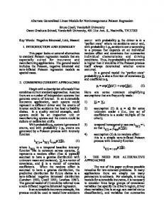
observations which seemed to be potentially dangerous in the model containing the whole set of variables. Probably, this outlyingness was due to some explanatory variables, which were not retained in the final model. For the final model as presented in Table 5, we investigate the sensitivity of Mallows quasi-likelihood tests compared to classical tests by considering the following procedure: we let the response of the observation receiving the lowest weight in the estimation of the final model, namely observation 110, span the range of values from 0 to 6. These values cover the range of the response in the sample. In each situation, we test the null hypothesis that the coefficient corresponding to the variable habitat is equal to 0. The p-values of these tests are represented in Figure 1. [Figure 1 about here.] The p-value of the robust test (c = 1.6) is stable, irrespective to the response value taken by observation 110. This p-value ranges from 2.6 to 3.3%. On the other hand, the p-value of the classical test (c = ∞), varies much more: from 2.3 to 6.5%, giving rise to a different model choice, if the decision rule is set at 5%. Moreover, by letting observation 110 take arbitrarily large values, the p-value of the robust test is bounded, whereas the p-value of the classical test continues to increase.
6
Conclusion
In this paper we proposed a natural class of robust testing procedures for generalized linear models. They are a valuable complement to classical techniques and are more reliable in the presence of outlying points and other deviations from the assumed model. Further research includes the extension of these procedures to generalized estimating equations and to nonparametric models like generalized additive models. 18
A
Fisher consistency correction
We derive the constant n
1 X £ ¡ Yi − µi ¢¤ 1 a(β) = E ψc 1/2 µ0i , 1/2 n i=1 V (µi ) V (µi ) £ ¡ i −µi ¢¤ . for binomial and Poisson models, which reduces to the computation of E ψc VY1/2 (µi ) Let us define j1 = bµi − cV 1/2 (µi )c, and j2 = bµi + cV 1/2 (µi )c.
The binomial model states that Yi ∼ B(mi , pi ), so that E[Yi ] = µi = mi pi and
i −µi . Then we have V[Yi ] = µi mm i
∞ X £ ¡ Yi − µi ¢¤ ¡ j − µi ¢ E ψc 1/2 = P(Yi = j)1I{j∈[0,mi ]} ψc 1/2 V (µi ) V (µi ) j=−∞ ¡ ¢ = c P(Yi ≥ j2 + 1) − P(Yi ≤ j1 ) ¤ µi £ ˜i ≤ j2 − 1) − P(j1 + 1 ≤ Yi ≤ j2 ) , + P(j ≤ Y 1 V 1/2 (µi )
with Y˜i ∼ B(mi − 1, pi ).
The Poisson model states that Yi ∼ P(µi ), and hence E[Yi ] = V (µi ) = µi . Then,
∞ X ¡ j − µi ¢ £ ¡ Yi − µi ¢¤ = P(Yi = j)1I{j≥0} ψc 1/2 E ψc 1/2 V (µi ) V (µ ) i j=−∞ ¡ ¢ ¤ µi £ = c P(Yi ≥ j2 + 1) − P(Yi ≤ j1 ) + 1/2 P(Yi = j1 ) − P(Yi = j2 ) . V (µi )
B
Asymptotic variance
We first determine the matrix Q(ψ c , F ) in the particular situation of Mallows quasilikelihood estimator. Using its definition, we have £¡ Q(ψ c , F ) = E ψc (r)w(x) =
1 V
1/2 (µ)
¢¡ µ0 − a(β) ψc (r)w(x)
1 T X AX − a(β)a(β)T , n
19
1 V
1/2 (µ)
µ0 − a(β)
¢T ¤
1 where A is the diagonal matrix with elements ai = E[ψc (ri )2 ]w2 (xi ) V (µ ( ∂µi )2 , since i ) ∂ηi ¡ i¢ ∂ xi . In the same manner, writing s(y, x, β) = ∂β µ0i = ∂µ log h(yi |xi , µi ), we derive ∂ηi
the expression of M (ψ c , F ),
£¡ M (ψ c , F ) = E ψc (r)w(x) = =
1 n
n X i=1
1 V
1/2 (µ)
¢ ¤ µ0 − a(β) s(y, x, β)T
£ ¤ ∂ 1 E ψc (ri ) log h(yi |xi , µi ) 1/2 w(xi )µ0i µ0T i ∂µi V (µi )
1 T X BX, n
i 2 ). where B is the diagonal matrix with elements bi = E[ψc (ri ) ∂µ∂ i log h(yi |xi , µi )] V 1/21(µi ) w(xi )( ∂µ ∂ηi
So, the determination of the asymptotic variance of a Mallows quasi-likelihood estimator involves the computation of the diagonal terms of the matrices A and B. We determine the three terms:
∂ −1 g (ηi ), ∂ηi
E[ψc (ri )2 ], and E[ψc (ri ) ∂µ∂ i log h(yi |xi , µi )]
for binomial and Poisson models. For the binomial model with logit link exp(ηi ) ∂ −1 , g (ηi ) = mi ∂ηi (1 + exp(ηi ))2 and ¡ ¢ £ ¡ Yi − µi ¢¤ = c2 P(Y ≤ j1 ) + P(Y ≥ j2 + 1) + E ψc2 1/2 V (µi ) 1 h 2 + π mi (mi − 1)P(j1 − 1 ≤ Y˜˜ ≤ j2 − 2) + V (µi ) i + (µi − 2µ2i )P(j1 ≤ Y˜ ≤ j2 − 1) + i 2 + µi P(j1 + 1 ≤ Y ≤ j2 ) , with Y ∼ B(mi , πi ), Y˜ ∼ B(mi − 1, πi ) and Y˜˜ ∼ B(mi − 2, πi ).
20
∂ ∂µi
log h(yi |xi , µi ) being equal to
Yi −µi , V (µi )
we have
£ ¤ £ ¡ Yi − µ i ¢ Yi − µ i ¤ ∂ E ψc (ri ) log h(yi |xi , µi ) = E ψc 1/2 = ∂µi V (µi ) V (µi ) i cµi h ˜ ˜ P(Yi ≤ j1 ) − P(Yi ≤ j1 − 1) + P(Yi ≥ j2 ) − P(Yi ≥ j2 + 1) + = V (µi ) h 1 + 3/2 π 2 mi (mi − 1)P(j1 − 1 ≤ Y˜˜i ≤ j2 − 2) V (µi ) i i 2 2 ˜ +(µi − 2µ )P(j1 ≤ Yi ≤ j2 − 1) + µ P(j1 + 1 ≤ Yi ≤ j2 ) . i
i
For the Poisson model, we use the log-link ηi = g(µi ) = log(µi ) which leads to ∂ −1 g (ηi ) ∂ηi
= exp(ηi ). We also have
¡ ¢ £ ¡ Yi − µi ¢¤ = c2 P(Yi ≤ j1 ) + P(Yi ≥ j2 + 1) + E ψc2 1/2 V (µi ) 1 h 2 + µ P(j1 − 1 ≤ Yi ≤ j2 − 2) + (µ − 2µ2 )P(j1 ≤ Yi ≤ j2 − 1) V (µ) i + µ2 P(j1 + 1 ≤ Yi ≤ j2 ) . The score function equals
∂ ∂µi
log h(yi |xi , µi ) =
Yi −µi µi
=
Yi −µi , V (µi )
so that
¤ £ ¡ Yi − µ i ¢ Yi − µ i ¤ £ ∂ E ψc (ri ) log h(yi |xi , µi ) = E ψc 1/2 = ∂µi V (µi ) V (µi ) ¡ ¢ = c P(Yi = j1 ) + P(Yi = j2 ) + ¡ ¢ 1 2 + P(Y = j − 1) − P(Y = j ) − P(Y = j − 1) + P(Y = j ) + µ i 1 i 1 i 2 i 2 i V 3/2 (µi ) + µi P(j1 ≤ Yi ≤ j2 − 1).
C
Conditions for Robust Quasi-deviance Tests
[C1]: Denote by Dn the set of all sample points zi , i = 1, . . . , n for which the secondorder derivatives ∂ 2 QM (zi , β)/∂βj ∂βk , i = 1, . . . , n; j, k = 1, . . . , p exist and are continuous functions of β. It is assumed that limn→∞ Pβ (Dn ) = 1. 21
[C2]: For any z ∈ Dn , any positive value δ, and any β 1 denote by ηjk (z, β 1 , δ) the
least upper bound and by γjk (z, β 1 , δ) the greatest lower bound of ∂ 2 QM (z, β)/∂βj ∂βk , with respect to β in the β interval ||β 1 − β|| ≤ δ. Moreover, assume that for any sequence {δn } for which limn→∞ δn = 0, £ ¤ £ ¤ £ ¤ lim Eβ ηjk (z, β, δn ) = lim Eβ γjk (z, β, δn ) = Eβ ∂ 2 QM (z, β)/∂βj ∂βk ,
n→∞
n→∞
£ 2 ¤ and that there exists a positive ² such that the expectations Eβ ηjk (z, β, δ) £ 2 ¤ and Eβ γjk (z, β, δ) are bounded functions of β and δ for all β and δ < ². These conditions are obtained by replacing log f (z, β) by QM (z, β) in the corresponding classical results for the likelihood ratio test; cf. Rao (1973), Wald (1943).
D
Proof of Proposition 1
First, we derive the asymptotic equivalent quadratic form of ΛQM . The proof follows the same lines as in the classical theory. The first step of the proof consists in approximating ΛQM under conditions [C1][C2] by √
√ ˆ − β) ˙ T M (ψ, F ) n(β ˆ − β), ˙ n(β
(14)
via a Taylor expansion and by making use of Slutsky’s theorem. Then, under H0 and by the asymptotic properties of M-estimators which hold under conditions (A.1)(A.9) of Heritier and Ronchetti (1994), the following distribution equality holds asymptotically √
D ˆ − β) ˙ ∼ n(β
¢ √ ¡ −1 ˜ + (ψ, F ) Ln , n M (ψ, F ) − M 22
(15)
where Ln =
1 n
Pn
i=1
ψ(yi , µi ) is such that
√
¡ ¢ nLn ∼ N 0, Q(ψ, F ) . Putting (15)
in (14), and taking into account the symmetry of M (ψ, F ), we finally have, as n → ∞,
D
ΛQM ∼ nLTn C(ψ, F )Ln .
(16)
(16) can be rewritten as D
ΛQM ∼ nRTn(2) M (ψ, F )22.1 Rn(2) , where M (ψ, F )22.1 = M (ψ, F )22 − M (ψ, F )12 M (ψ, F )−1 11 M (ψ, F )12 , and ¡ ¢ distributed according to N 0, M −1 (ψ, F )Q(ψ, F )M −1 (ψ, F ) .
√
nRn is
Finally, from (16) we conclude that
ΛQM ∼
q X
di Ni2 ,
i=1
where di are the q positive eigenvalues of Q(ψ, F )C(ψ, F ) and N1 , . . . , Nq are independent standard normal variables. Thus, the distribution of ΛQM is a linear combination of χ2 random variables with 1 degree of freedom.
E
Proof of Proposition 2
By using (11) and by standard results on the distribution of quadratic forms in normal variables, we can say that the statistic nUTn AUn is asymptotically distributed P √ as qi=1 di χ21 (ξi2 ), with ξ(²) = (ξ1 (²), . . . , ξq (²))T = nP U(F²,n ). Notice that the
distribution depends only on the ξi2 (²) (see Johnson and Kotz (1970), Chapter 29).
Moreover, up to O(1/n), we have that α(F²,n ) = 1 − Hd1 ,...,dq (η1−α0 ; λ(²)), with ¡ ¢ λ(²) = diag(ξ(²)ξ(²)T ) = n diag P U(F²,n )U(F²,n )T P T . 23
Let b(²) = −Hd1 ,...,dq (η1−α0 ; λ(²)). Then, up to O(1/n), we have 1 α(F²,n ) − α0 = b(²) − b(0) = ²b0 (0) + ²2 b00 (0) + o(²2 ). 2 But b0 (0) = κT ·
³ h∂ i ´ ∂ ¯¯ λ¯ = 2nκT · diag P U(F²,n ) U(Fβ0 )P T = 0, ∂² ²=0 ∂² ²=0
because U(Fβ0 ) = 0.
We also have that ´ i ³ h∂ ∂ 2 ¯¯ ∂ T T T λ P U(F ) U(F ) = κ · 2n diag P ¯ ²,n ²,n ∂²2 ²=0 Z ∂² ∂² ²=0 ´T ´ ´ ³Z ³ ³ T IF(z;U, Fβ0 )dG(z) P T , IF(z;U, Fβ0 )dG(z) = 2κ · diag P
b00 (0) = κT ·
by using again the fact that U(Fβ0 ) = 0 and because
¯
∂ U(F²,n )¯²=0 ∂²
(see Hampel et al., 1986, p. 83). This completes the proof.
=
R
IF(z; U, Fβ0 ) √1n dG(z)
Acknowledgments Eva Cantoni (
[email protected]) is maˆıtre-assistante and Elvezio Ronchetti (
[email protected]) is Professor, Department of Econometrics, CH-1211 Geneva 4, Switzerland. The authors would like to thank the Editor, the Associate Editor, the referees, P. Rousseeuw and M.-P. Victoria-Feser for their valuable suggestions, and A. Welsh for providing the data analyzed in Section 5.2. The hospitality of Stanford (E. C.) and MIT (E. R.) during the revision of the manuscript is gratefully acknowledged.
24
References Bednarski, T. (1993), “Fr´echet Differentiability of Statistical Functionals and Implications to Robust Statistics,” in New Directions in Statistical Data Analysis and Robustness, eds. Morgenthaler, S., Ronchetti, E., and Stahel, W. A., Basel/Cambridge, MA: Birkhaeuser, pp. 25–34. Carroll, R. J. and Welsh, A. H. (1988), “A Note on Asymmetry and Robustness in Linear Regression,” The American Statistician, 42, 285–287. Clarke, B. R. (1986), “Nonsmooth Analysis and Frechet Differentiability of M functionals,” Probability Theory and Related Fields, 73, 197–209. Davies, R. B. (1980), “[Algorithm AS 155] The Distribution of a Linear Combination of χ2 Random Variables (AS R53: 84V33 P366- 369),” Applied Statistics, 29, 323– 333. Farebrother, R. W. (1990), “[Algorithm AS 256] The Distribution of a Quadratic Form in Normal Variables,” Applied Statistics, 39, 294–309. Hampel, F. R. (1974), “The Influence Curve and Its Role in Robust Estimation,” Journal of the American Statistical Association, 69, 383–393. Hampel, F. R., Ronchetti, E. M., Rousseeuw, P. J., and Stahel, W. A. (1986), Robust Statistics: The Approach Based on Influence Functions, New York: Wiley. Hanfelt, J. J. and Liang, K.-Y. (1995), “Approximate Likelihood Ratios for General Estimating Functions,” Biometrika, 82, 461–477.
25
He, X. and Simpson, D. G. (1993), “Lower Bounds for Contamination Bias: Globally Minimax Versus Locally Linear Estimation,” The Annals of Statistics, 21, 314– 337. He, X., Simpson, D. G., and Portnoy, S. L. (1990), “Breakdown Robustness of Tests,” Journal of the American Statistical Association, 85, 446–452. Heritier, S. and Ronchetti, E. (1994), “Robust Bounded-influence Tests in General Parametric Models,” Journal of the American Statistical Association, 89, 897–904. Heyde, C. C. (1997), Quasi-Likelihood and its Application, Berlin/New York: Springer-Verlag. Huber, P. J. (1967), “The Behavior of the Maximum Likelihood Estimates under Nonstandard Conditions,” in Proceedings of the Fifth Berkeley Symposium on Mathematical Statistics and Probability, pp. 221–233. — (1981), Robust Statistics, New York: Wiley. Imhof, J. P. (1961), “Computing the Distribution of Quadratic Forms in Normal Variables,” Biometrika, 48, 352–363. Johnson, N. L. and Kotz, S. (1970), Continuous Univariate Distributions, vol. 2, Boston; Geneva, IL: Houghton-Mifflin. K¨ unsch, H. R., Stefanski, L. A., and Carroll, R. J. (1989), “Conditionally Unbiased Bounded-influence Estimation in General Regression Models, With Applications to Generalized Linear Models,” Journal of the American Statistical Association, 84, 460–466.
26
Lindenmayer, D. B., Cunningham, R. B., Tanton, M. T., Nix, H. A., and Smith, A. P. (1991), “The Conservation of Arboreal Marsupials in the Montane Ash Forests of the Central Highlands of Victoria, South-East Australia: III. The Habitat Requirements of Leadbeater’s Possum Gymnobelideus leadbeateri and Models of the Diversity and Abundance of Arboreal Marsupials,” Biological Conservation, 56, 295–315. Lindenmayer, D. B., Cunningham, R. B., Tanton, M. T., Smith, A. P., and Nix, H. A. (1990), “The Conservation of Arboreal Marsupials in the Montane Ash Forests of the Victoria, South-East Australia, I. Factors Influencing the Occupancy of Trees with Hollows,” Biological Conservation, 54, 111–131. Markatou, M., Basu, A., and Lindsay, B. G. (1998), “Weighted Likelihood Equations With Bootstrap Root Search,” Journal of the American Statistical Association, 93, 740–750. Markatou, M. and He, X. (1994), “Bounded Influence and High Breakdown Point Testing Procedures in Linear Models,” Journal of the American Statistical Association, 89, 543–549. McCullagh, P. and Nelder, J. A. (1989), Generalized Linear Models, London: Chapman & Hall, 2nd ed. Morgenthaler, S. (1992), “Least-absolute-deviations Fits for Generalized Linear Models,” Biometrika, 79, 747–754. Pearson, E. S. (1959), “Note on the Distribution of Non-central χ2 ,” Biometrika, 46, 364.
27
Phelps, K. (1982), “Use of the Complementary log-log Function to Describe Doseresponse Relationships in Insecticide Evaluation Field Trials,” in Lecture Notes in Statistics, No. 14. GLIM.82: Proceedings of the International Conference on Generalized Linear Models, ed. Gilchrist, R., Berlin/New York: Springer-Verlag. Pregibon, D. (1982), “Resistant Fits for Some Commonly Used Logistic Models With Medical Applications,” Biometrics, 38, 485–498. Preisser, J. S. and Qaqish, B. F. (1999), “Robust Regression for Clustered Data with Applications to Binary Regression,” Biometrics, 55, 574–579. Rao, C. R. (1973), Linear Statistical Inference, New York: Wiley, 2nd ed. Ronchetti, E. (1997), “Robustness Aspects of Model Choice,” Statistica Sinica, 7, 327–338. Ronchetti, E. and Staudte, R. G. (1994), “A Robust Version of Mallows’ C p ,” Journal of the American Statistical Association, 89, 550–559. Ronchetti, E. and Trojani, F. (2001), “Robust Inference with GMM Estimators,” Journal of Econometrics, 101, 36–79. Rousseeuw, P. J. and Leroy, A. M. (1987), Robust Regression and Outlier Detection, New York: Wiley. Ruckstuhl, A. F. and Welsh, A. H. (1999), “Robust Fitting of the Binomial Model,” Manuscript. Sommer, S. and Huggins, R. (1996), “Variable Selection using the Wald Test and a Robust Cp ,” Applied Statistics, 45, 15–29. 28
Staudte, R. G. and Sheather, S. J. (1990), Robust Estimation and Testing, New York: Wiley. Stefanski, L. A., Carroll, R. J., and Ruppert, D. (1986), “Optimally Bounded Score Functions for Generalized Linear Models With Applications to Logistic Regression,” Biometrika, 73, 413–424. Wald, A. (1943), “Test for Statistical Hypotheses Concerning Several Parameters when the Number of Observations is Large.” Transactions of the American Mathematical Society, 54, 426–482. Wedderburn, R. W. M. (1974), “Quasi-likelihood Functions, Generalized Linear Models, and the Gauss-Newton Method,” Biometrika, 61, 439–447. Weisberg, S. and Welsh, A. H. (1993), “Missing Links,” in New Directions in Statistical Data Analysis and Robustness, eds. Morgenthaler, S., Ronchetti, E., and Stahel, W. A., Basel/Cambridge, MA: Birkhaeuser, pp. 275–284. Williams, D. A. (1987), “Generalized Linear Model Diagnostics Using the Deviance and Single Case Deletions,” Applied Statistics, 36, 181–191.
29
0.06 0.03
pvalue 0.04
0.05
c=1.6 c=Inf
0
1
2
3 y110
4
5
6
Figure 1: Sensitivity curves of the p-value for Mallows quasi-likelihood tests with c = 1.6 (solid line) and c = ∞ (dashed line).
30
Intercept logdose block2 block1
Max. likelihood 1.480 (0.66) -1.817 (0.34) 0.843 (0.23) 0.542 (0.23)
Huber quasi-likelihood 1.939 (0.70) -2.049 (0.37) 0.685 (0.24) 0.450 (0.24)
Table 1: Estimation of β by maximum likelihood and by the Huber quasi-likelihood estimator with c = 1.2. Standard errors are indicated within parentheses.
31
NULL logdose block2 block1
Resid. Deviance 83.34 54.73 (0.000) 45.59 (0.003) 39.98 (0.018)
Resid. Huber quasi-deviance 60.46 39.94 (0.000) 35.21 (0.017) 32.74 (0.085)
Table 2: Residual deviance and residual Huber quasi-deviance with c = 1.2. p-values are indicated within parentheses.
32
Variable Intercept shrubs stumps stags bark acacia habitat eucalyptus nitens eucalyptus regnans eucalyptus delegatensis aspect NW-NE aspect NW-SE aspect SE-SW aspect SW-NW
Coefficient -0.8978 (-0.947) 0.0099 (0.012) -0.2514 (-0.272) 0.0402 (0.040) 0.0400 (0.040) 0.0178 (0.018) 0.0714 (0.072) 0 (0) -0.020 (-0.015) 0.127 (0.115) 0 (0) 0.0601 (0.067) 0.0949 (0.117) -0.5079 (-0.489)
Standard Error 0.2682 (0.265) 0.0222 (0.022) 0.2876 (0.286) 0.0113 (0.011) 0.0145 (0.014) 0.0107 (0.011) 0.0385 (0.038) (-) 0.1938 (0.192) 0.2738 (0.272) (-) 0.1913 (0.190) 0.1920 (0.190) 0.2505 (0.247)
Table 3: Coefficients estimation and corresponding standard errors for the Poisson model with log-link of the possum dataset.
33
shrubs stumps stags bark acacia habitat eucalyptus regnans eucalyptus delegatensis eucalyptus nitens aspect NW-NE aspect NW-SE aspect SE-SW aspect SW-NW
Classical QL Robust QL 0.0871 0.3642 0.0646 0.2988 0.0000 0.0000 0.0035 0.0039 0.0002 0.0009 0.0500 0.0443 0.8754 0.8030 0.8591 0.8074 0.5681 0.6461 0.8336 0.9100 0.2612 0.3462 0.1996 0.1646 0.0012 0.0023
Table 4: p-values of a forward stepwise procedure for the Poisson model with log-link of the possum dataset.
34
Variable Coefficient Intercept -0.7981 (-0.8213) stags 0.0406 (0.0410) bark 0.0410 (0.0406) habitat 0.0143 (0.0136) acacia 0.0776 (0.0782) aspect SW-NW -0.6044 (-0.5968)
Standard Error 0.2030 (0.2000) 0.0104 (0.0103) 0.0126 (0.0125) 0.0098 (0.0097) 0.0371 (0.0367) 0.2121 (0.2086)
Table 5: Coefficients estimation and corresponding standard errors for the final Poisson model with log-link of the possum dataset.
35