Arun Ayyarâ, Michael Lentmaierâ , K. Giridharâ and Gerhard Fettweisâ . âDepartment. of ... order approximation of the Middleton model is an Ç«-Gaussian.
Robust Initial LLRs for Iterative Decoders in Presence of Non-Gaussian Noise Arun Ayyar∗, Michael Lentmaier† , K. Giridhar∗ and Gerhard Fettweis† ∗ Department.
of Electrical. Engg, Indian Institute of Technology Madras, Chennai-600036, India. Email: {arun ayyar, giri}@tenet.res.in † Vodafone Chair, Mobile Communications Systems, Technische Universit¨at Dresden, Germany. Email: {michael.lentmaier, fettweis}@ifn.et.tu-dresden.de
Abstract—We consider the decoding of LDPC codes in presence of non-Gaussian noise, especially a set of ǫ-mixture models. For each of these models, the optimal LLRs are presented. We study the performance degradation due to the use of incorrect LLR in presence of a given noise model. Without modifying the existing LDPC decoder, we propose robust initial LLR which require minimum knowledge about the underlying noise model and are computationally less complex. Since BER simulations are computationally heavy, we use density evolution to compare the thresholds of different LLRs.
I. I NTRODUCTION In communication systems, noise is usually modeled as a Gaussian process. However some systems experience interference which is better characterised as impulsive noise. One example of such an environment is co-channel interference in reuse-1 OFDM systems such as 802.16d/e and LTE. In reuse-1 cellular systems, the main source of interference is the use of same sub-carriers at the same time in the neighboring cells/sectors. In 802.16d/e, the base stations are frequency synchronised and hence the subcarriers of the interfering user will fall exactly on the subcarrier of the desired user. The fraction of affected sub carriers depends on number of users, the geographical distance between the desired user and the interfering user, the channel between them and the channel between desired user and the base station. Hence only some of the subcarriers will be affected by the co-channel interference. Such noise will appear as impulsive noise in the frequency domain. Several models have been proposed for the impulsive noise in the literature. The most commonly used model is the Middleton class A model [1] which is composed of the mixture of a Rayleigh distribution for the impulse amplitude with Poisson distribution for occurrence of the impulses. A first order approximation of the Middleton model is an ǫ-Gaussian mixture model[2]. Another candidate for modelling impulsive noise are the symmetric alpha stable noise models. [3] proposes to use Cauchy-Gaussian(CGM) mixture model, which inspite of being simple can capture the algebraic tail. CGMs can be used to fit the Middleton Class B impulsive noise model, which includes alpha-stable noise as a special case [4]. The ǫ-mixture model with the contaminating pdf being double exponential is a limiting case of the Mertz model, which is
used to model impulsive noise in a telephone plant [5]. Low Density Parity-Check (LDPC) codes, invented by Gallager[6], achieve near capacity performance in a wide class of channels. In the present work, we consider the decoding of the LDPC codes in presence of the above mentioned noise models. Several approaches have been proposed in the literature for decoding of turbo codes. In presence of impulsive noise if the initial LLR (Log-likelihood Ratio)s are generated using the Gaussian assumption the performance degradation is significant [7]. If the true noise pdf is known, we can construct the initial LLRs based on the pdf. However, there are 3 different noise models available for the impulsive noise and even if the pdf is known estimation of the other parameters of the pdf is not an easy task. Several robust1 LLRs in presence of the above mentioned models have been studied in the literature in the context of turbo decoding without incorporating change in the existing decoders. In [8], authors propose Parametric-Cauchy LLR (PC-LLR) which was based on the Cauchy-Gaussian mixture model. [9] reduces the complexity of PC-LLR by applying the generalised likelihood principle [10]. We analyse the different initial LLRs for LDPC codes using the density evolution technique. The organisation of the paper is as follows: In Section II, we discuss the different noise models. Section III discusses different optimal initial LLRs. In Section IV we use density evolution to analyse the performance of the optimal LLRs in different noise models, in section V we study the performance of different robust LLRs and also propose a new LLR and finally in Section VI, we present conclusions. II. I MPULSIVE NOISE MODELS In this section we present the different noise models that we consider in this paper Contaminated Gaussian PDF(CG) 2
2
n − n2 ǫ 1 − ǫ − 2σ 2 e 2σnb e 1 +p fg (n) = p 2 2 2πσnb 2πσ1
(1)
2 where σnb > σ12 .
1 Robust is used to mean that the LLRs do not need the knowledge of the underlying pdf and all its parameters
where fn (x) can be any of the above mentioned noise models. The expressions for LLRs in presence of the above mentioned noise models for BPSK modulation can be written as follows:
Contaminated Laplacian PDF(CL) 2
x − ǫ 1 − ǫ − 2σ 2 fl (x) = p e 1 +p 2 e 2 2σnb 2πσ1
r
2 σ2 nb
|x|
(2)
Gaussian LLR (GLLR)
Contaminated Cauchy PDF(CC)
Considering fn (x) = √ 1
2πσ12
e
−
x2 2 2σ1
2
x 1 − ǫ − 2σ ǫγ 2 fc (x) = p e 1 + 2 2 π(γ + x2 ) 2πσ1
LG (yk ) =
(3)
−
(yk −1)
−
(yk −1)
2 2 e 2σ1 + √ ǫ 2 e 2σnb √1−ǫ 2πσnb 2πσ12 LCG (yk ) = log 2 (y +1)2 1−ǫ − (yk2σ+1) − k2 2 √ 2e 1 + √ ǫ 2 e 2σnb
2πσnb
2πσ1
(8)
Contaminated Laplacian LLR (CLLLR)
2Cg
Considering (2) as the noise, optimal LLR is r 2
Hence all the three noise models can be represented as : + ǫH
(7)
If the assumed noise pdf has distribution as in (1), then the optimal LLR for this noise is 2 2
where Cg = eCe = 1.78 is the exponential of the Euler constant Ce = 0.5772. Here, S0 is the geometric power of symmetric α-stable pdf. To keep the GSNR of the Cauchy pdf and the Gaussian pdf, we choose γ= √σnb [8]. 1−ǫ fn (x) = e 2πσ12
2y σ12
Contaminated Gaussian LLR (CGLLR)
Since the variance is not defined for the Cauchy pdf, as an alternate estimate of noise power,we chose Geometric-Signalto-Noise Ratio (GSNR). GSNR is defined as [7] � �2 A 1 (4) GSN R = 2Cg S0
2 − x2 2σ 1
,
(5)
LCL (yk ) = log
where H is any symmetric pdf. The considered choices of H are Gaussian, Laplacian and Cauchy pdfs. As seen from (5) the ǫ-mixture model has four unknowns • The contaminating pdf H • The variance σ1 Gaussian part of the pdf • The variance(or equivalent parameter) σnb of the contaminating heavy-tailed pdf • Percentage of samples ǫ from the heavy-tailed pdf For the co channel interference scenario, since all the factors are time varying, ǫ and σnb are time varying, hence difficult to estimate. The fraction of subcarriers ǫ affected can range from 0 ≤ ǫ < 0.5 with values greater than 0.3 occurring with very low probability. Chosen ranges for parameters are 2 1.0 ≤ σnb ≤ 4.0 and 0 < ǫ ≤ 0.3. We assume the knowledge 2 of σ1 .
− √1−ǫ 2 e 2πσ1
√1−ǫ 2 e
−
(yk −1) 2 2σ1
(yk +1)2 2σ2 1
+
√ǫ2 e 2σnb
+ √ǫ2 e 2σnb
2πσ1
−
−
r
2 σ2 nb
2 σ2 nb
|yk −1|
|yk +1|
(9)
Contaminated Cauchy LLR (CCLLR)
LCC (yk ) = log
√1−ǫ 2 e
−
(yk −1)2 2σ2 1
2πσ1
√1−ǫ 2 e 2πσ1
(y +1)2 − k 2 2σ 1
+ +
ǫγ π(γ 2 +(yk −1)2 ) ǫγ π(γ 2 +(yk +1)2 )
(10)
is the optimal LLR if (3) is the assumed noise pdf. Fig. 1 illustrates the ineffectiveness of the GLLR in the considered noise models. Assumed noise model is contami2 nated Gaussian noise with σnb = 4.0 and ǫ = 0.1. The ideal LLR in this case would be CGLLR with the true parameters. We use regular (3,6) LDPC convolutional codes [11],[12] with memory length of 1025 for simulation. The decoding algorithm used is belief propagation with 100 iterations. From Fig. 1 it is clear that GLLR cannot be used for the considered noise models. We shall study the performance of other optimal LLRs when the assumed noise pdf is not the same as the pdf assumed for the LLR. E.g. let us assume that the actual noise pdf is 2 Contaminated Gaussian pdf with parameters σnb = 4.0 and ǫ = 0.1. We would like to quantify the performance degradation when we use CLLLR or CCLLR instead of CGLLR, which is the optimal LLR in this case. BER simulations for all the combinations of noise and LLRs would take a lot of time. Performance of the LDPC codes can also be analysed using the density evolution. We shall use density evolution
III. O PTIMAL I NITIAL LLR S Let xk be the k th transmitted M-QAM symbol. nk be samples from any of the above mentioned noise pdfs fn . At the receiver the received symbol yk is yk = xk +nk . Let S = s0 , s1 , .., sn , where n = 2M − 1, be the set of all M-QAM constellation points. s+ j is subset of S containing constellation points with 1 in the j th position s− j is subset of S containing constellation points with 0 in the j th position The log-likelihood ratio of the j th coded bit in the k th symbol is defined as P ! fn (yk − xk ) xk ∈s+ j (6) L(yk,j ) = log P xk ∈s− fn (yk + xk ) j
2
0
10
CGLLR GLLR
1 2
0.12
2
−1
10
0.1 0.08
p(L(yk))
−2
BER
10
0.06
1
−3
10
0.04 −4
Threshold
10
0.02 0 −5
−5
10
0
0.5
1
1.5
2
2.5
3
3.5
−4
−3
−2
SNR 2 = 4.0, regular (3,6) Fig. 1. Contaminated Gaussian noise, ǫ = 0.1, σnb LDPC convolutional codes with ms = 1025. Decoding algorithm is belief propagation with iterations = 100. The threshold for regular (3,6) LDPC convolutional codes is at 2.45 dB shown by the vertical line.
−1
0
L(yk)
1
2
3
4
5
Fig. 2. Pdf of the CLLLR for Contaminated Laplacian noise with parameters 2 = 4.0 , σ 2 = 0.5 ǫ = 0.1, σnb 1
and a candidate LLR, the threshold is defined as: σ1∗ = max(σ1 ) :
for comparing the performance of different LLRs for a given noise pdf.
Pb (σ1 ) → 0
We have tabulated thresholds for regular (3,6) LDPC codes for different combinations of the above mentioned LLR and noises. Since our main objective is to compare different LLRs, the thresholds are accurate up to only two decimal places Eb ∗ in dB after the decimal point. All tables contain the N 0 corresponding to σ1∗ The approximate thresholds for Contaminated Gaussian noise are as below:
IV. D ENSITY E VOLUTION For the LDPC codes, it has been observed that as the blocklength tends to infinity, arbitrarily low probability of error can be achieved if the variance of the noise is less than a certain value, called the threshold. If the variance of noise is more than the threshold, the probability of error will be greater than a positive constant. Richardson and Urbanke calculated the threshold for a variety of channels [13],[14] for message passing algorithms, using density evolution. Calculating thresholds for most channels other than Binary Erasure Channel(BEC) is a computationally expensive task. [15] proposed discrete density evolution for reducing the computational complexity of density evolution technique. The Extrinsic Information Transfer(EXIT) charts[16] are based on the assumption that the the extrinsic information exchanged between the two decoders has a Gaussian distribution. Density evolution technique does not make any assumption about the distribution of the messages passed between the check nodes and bit nodes. Pdfs of the initial LLRs in presence of the ǫ−mixture noise models will most likely not be Gaussian. Fig.2 shows the initial pdf of LLRs when the input noise is Contaminated Laplacian and CLLLR is used for decoding. The 2 = 4.0 and ǫ = 0.1 parameters of the pdf are σnb T HRESHOLDS FOR THE ǫ- MIXTURE
lim
iterations→∞
TABLE I A PPROXIMATE THRESHOLDS FOR C ONTAMINATED G AUSSIAN (CG) NOISE 2 σnb 1 1 2 2 4 4
ǫ 0.1 0.3 0.1 0.3 0.1 0.3
LCG 1.25 1.68 1.84 4.43 2.46 7.99
LCL 1.26 1.75 1.86 4.65 2.49 8.45
LCC 1.29 1.94 1.90 5.05 2.53 9.14
TABLE II A PPROXIMATE THRESHOLDS FOR C ONTAMINATED L APLACIAN NOISE 2 σnb 1 1 2 2 4 4
MODELS
ǫ 0.1 0.3 0.1 0.3 0.1 0.3
LCG 1.22 1.59 1.63 3.21 2.04 5.03
LCL 1.20 1.45 1.59 2.99 2.01 4.79
LCC 1.23 1.54 1.61 3.06 2.02 4.89
From Table I, the threshold for CGLLR in presence of 2 contaminated Gaussian noise with σnb = 4.0 and ǫ = 0.1 is 2.45 dB. Fig.1 shows that the simulation of the regular (3,6) LDPC convolutional codes with same noise parameters and CGLLR is quite close to the calculated threshold at BER = 10−5 .
Density evolution can be used to find the maximum variance of channel noise which is likely to be corrected by a particular ensemble using the message-passing algorithm. For the above mentioned models, we define threshold as following: For a given ensemble with block length → ∞, for a fixed σnb , ǫ 3
Parametric Cauchy LLR (PCLLR) 8 6 4
1 2 3 4
CGLLR CLLLR GLLR CCLLR
3
4
2
|yk −1|2
2πσ1
k
L(y )
2
−
0.7 2σ2 1 + √2πσ12 e LP C (yk ) = log 2 (y +1) − k √0.7 2 e 2σ12 +
1
0
0.3∗1.06 π((1.06)2 +(yk −1)2 ) 0.3∗1.06 π((1.06)2 +(yk +1)2 )
(11)
[9] reduces the dependence on γ and ǫ in (10) by using the generalised likelihood principle.
−2 −4
Generalised Likelihood Metric (GLR)
−6 −6
−5
−4
Fig. 3.
−3
−2
−1
0 yk
1
2
3
4
5
LGLR (yk ) = log
6
TABLE III A PPROXIMATE THRESHOLDS FOR C ONTAMINATED C AUCHY NOISE ǫ 0.1 0.3 0.1 0.3 0.1 0.3
LCL 1.49 2.41 1.68 3.22 1.91 4.28
!
(12)
Hence GLR does not need any of the 4 afore mentioned parameters. However seen from (12) it is clear that when yk → ±1, LGLR(yk ) → ∞. Since knowledge of σ1 is assumed, [17] reintroduces σ1 into (12) as shown below.
L(yk )vs yk for different optimal initial LLRs
2 σnb 1 1 2 2 4 4
1 π(yk −1)2 1 π(yk +1)2
LCC 1.40 2.07 1.63 2.99 1.89 4.15
Parametric Generalised Log Likelihood Ratio (PGLLR)
LP G (yk ) = log
�
P (yk /xk = 1) P (yk /xk = −1)
�
(13)
where t = πσ1 2 P (yk /xk = i) = π(yk1−i)2 , 0 < π(yk1−i)2 < t 1 P (yk /xk = i) = t , π(yk −i)2 > t for i∈{1, −1} Here t limits the value of numerator and the denominator in (13). It was shown in [17] that PGLLR is has better performance than GLR, so we consider only PGLLR. We present the approximate thresholds in dB for all the three noise models in presence of PCLLR and PGLLR. In each case, PCLLR and PGLLR are compared with the optimal LLR for the given noise with true parameters.
As seen from Table I, CLLLR and CCLLR are within 1.5 dB from CGLLR, which is the optimal LLR for Contaminated Gaussian noise. From Table II it is seen that CGLLR and CCLLR are within 1 dB from CLLLR. Hence in the CG and CL noises, all the three optimal LLRs show a maximum degradation about 1 dB. However, in CC noise, for some of 2 the σnb and ǫ combinations the Pb does not tend to zero as iterations → ∞. Hence we could not find threshold in these cases. As seen from Fig.3 the shape of LG (yk ) vs yk is a straight line. Hence larger values of yk are assigned higher reliability. While in case of CCLLR yk → ∞ , L(yk ) → 0, i.e, larger values of yk are given lower reliability. So GLLR does not perform well in these noise cases. In case of CGLLR we see that yk → ∞, L(yk ) is a straight line. So it does not perform well in heavier tailed pdf like contaminated Cauchy. So from Table I, II and III we can conclude that, either CLLLR or CCLLR with the correct parameter values can be used in the other noise cases too with some performance degradation.
TABLE IV A PPROXIMATE THRESHOLDS FOR PCLLR AND PGLLR IN C ONTAMINATED G AUSSIAN (CG), C ONTAMINATED L APLACIAN (CL) AND C ONTAMINATED C AUCHY (CC) NOISES CG 2 σnb 1 1 2 2 4 4
V. ROBUST I NITIAL LLR S In this section we shall study the performance of some of the LLRs which do not need the true value of the parameters of the underlying noise pdf. We assume that out of the 4 parameters of the ǫ-mixture models, only σ12 can be estimated. Hence we study other alternative LLRs which need true value of σ12 . In [8] the author proposes Parametric Cauchy LLR by fixing the parameters of CCLLR.
ǫ 0.1 0.3 0.1 0.3 0.1 0.3
LP C 1.55 2.07 2.04 4.97 2.53 9.13
CL LP G 2.21 2.79 2.59 4.89 2.95 9.15
LP C 1.46 1.67 1.77 3.08 2.11 4.89
CC LP G 2.11 2.38 2.36 3.47 2.63 5.26
LP C 1.58 2.15 1.78 3.01 2.01 4.15
LP G 2.20 2.74 2.37 3.45 2.56 4.41
Table IV shows the thresholds for PCLLR and PGLLR. Comapring with Table I, II and III, it is seen that PGLLR is within 1.5dB from CGLLR, within 0.5 dB from CLLLR and within 0.3 dB from CCLLR. PCLLR and PGLLR don’t need 2 the knowledge of the thick-tailed pdf, ǫ and σnb . Moreover PGLR has a simpler expression than PCLLR. 4
PGLLR-2
by the LLRs is the variance of the Gaussian noise. Without requiring any estimation of the interference pdfs and their parameters, the thresholds of the robust LLR are within 0.51 dB in all the three considered noise models for regular (3,6) LDPC codes. For iterative interference cancellation, these LLRs can be used as replacement of the standard GLLR to improve the initial iterations. Although we have considered only LDPC codes in this paper, the proposed LLRs can be used for other iterative decoders too.
σ12
In (13),which is a modification of (12), is used as a limiting value. We propose another method of incorporating σ12 in (12). ! 1 LP G−2 (yk ) = log
π(yk −1)2 +σ12 1 π(yk +1)2 +σ12
Threshold comparison for PGLR and PGLR-2 for Contaminated Laplacian and Contaminated Cauchy noises is given in Table VII. TABLE V C OMPARISON OF APPROXIMATE THRESHOLDS BETWEEN LP G LP G−2 FOR C ONTAMINATED L APLACIAN NOISE 2 σnb 1 1 2 2 4 4
ǫ 0.1 0.3 0.1 0.3 0.1 0.3
Cont. Lap LP G LP G−2 2.11 2.09 2.38 2.06 2.36 2.10 3.47 3.33 2.63 2.39 5.26 4.99
R EFERENCES [1] D. Middleton, “Statistical-Physical Models of Electromagnetic Interference,” Electromagnetic Compatibility, IEEE Transactions on, pp. 106– 127, 1977. [2] K. Vastola, “Threshold Detection in Narrow-Band Non-Gaussian Noise,” IEEE Transactions on Communications, vol. 32, no. 2, pp. 134–139, 1984. [3] A. Swami, “Non-gaussian mixture models for detection and estimation in heavy-tailed noise,” Acoustics, Speech, and Signal Processing, 2000. ICASSP’00. Proceedings. 2000 IEEE International Conference on, vol. 6, 2000. [4] D. Middleton, “Non-Gaussian noise models in signal processing for telecommunications: New methods an results for class A and class B noise models,” Information Theory, IEEE Transactions on, vol. 45, no. 4, pp. 1129–1149, 1999. [5] J. Miller and J. Thomas, “Detectors for discrete-time signals in nongaussian noise,” Information Theory, IEEE Transactions on, vol. 18, no. 2, pp. 241–250, 1972. [6] R. G. Gallager, “Low-Density Parity-Check Codes,” Ph.D. dissertation, MIT, 1963. [7] T.C.Chuah, “Robust iterative decoding of turbo codes in heavy-tailed noise,” vol. 152. IEE, Feb 2005, pp. 29–38. [8] S. Kalyani and K.Giridhar, “Interference Mitigation in Turbo-Coded OFDM Systems Using Robust LLRs.” IEEE, May 2008, pp. 646–651. [9] A. Ayyar and K.Giridhar, “Robust LLRs using the Generalised Likelihood Principle,” selected for publication at National Communications Conference’09, Guwahati, Jan 2009. [10] B. Peric, M. Souryal, E. Larsson, and B. Vojcic, “Soft decision metrics for turbo-coded FH M-FSK ad hoc packet radio networks,” Vehicular Technology Conference, 2005. VTC 2005-Spring. 2005 IEEE 61st, vol. 2, pp. 724–727 Vol. 2, May-1 June 2005. [11] A. Jimenez Felstrom and K. Zigangirov, “Time-varying periodic convolutional codes with low-density parity-check matrix,” Information Theory, IEEE Transactions on, vol. 45, no. 6, pp. 2181–2191, Sep 1999. [12] A. Pusane, A. Feltstrom, A. Sridharan, M. Lentmaier, K. Zigangirov, and D. Costello, “Implementation aspects of LDPC convolutional codes,” Communications, IEEE Transactions on, vol. 56, no. 7, pp. 1060–1069, July 2008. [13] T. J. Richardson and R. L. Urbanke, “The capacity of low-density paritycheck codes under message-passing decoding,” IEEE Transactions on Information Theory, vol. 47, no. 2, pp. 599–618, 2001. [14] T. Richardson, M. Shokrollahi, and R. Urbanke, “Design of capacityapproaching irregular low-density parity-check codes,” Information Theory, IEEE Transactions on, vol. 47, no. 2, pp. 619–637, Feb 2001. [15] S.-Y. Chung, J. Forney, G.D., T. Richardson, and R. Urbanke, “On the design of low-density parity-check codes within 0.0045 dB of the Shannon limit,” Communications Letters, IEEE, vol. 5, no. 2, pp. 58–60, Feb 2001. [16] S. ten Brink, “Convergence behavior of iteratively decoded parallel concatenated codes,” Communications, IEEE Transactions on, vol. 49, no. 10, pp. 1727–1737, 2001. [17] A. Ayyar and K.Giridhar, “Robust, Low Complexity LLRs for Interference Mitigation in Reuse-1 OFDM,” World Wireless Research Forum, Stockholm , Oct, 2008.
AND
Cont Cauchy LP G LP G−2 2.20 1.90 2.74 2.39 2.37 2.08 3.45 3.20 2.56 2.29 4.41 4.33
We can see that the threshold of PGLR-2 is better than PGLR by about 0.1-0.3 dB. From Table II,IV and V, we 0
10
PGLLR−2 PGLLR PCLLR CLLLR
1 2 3
−1
10
4
−2
BER
10
4 3
−3
10
2 1
−4
10
−5
10
1
1.5
2
2.5
3
3.5
Eb/No Fig. 4. BER comparison for CLLLR,PCLLR,PGLLR and PGLLR-2 for CL 2 = 4.0, regular (3,6) LDPC convolutional noise with parameters ǫ = .1, σnb codes with ms = 1025
see that BER curves shown in Fig. 4 are consistent with the approximate threshold values presented for CL noise with 2 parameters ǫ = 0.1, σnb = 4.0. VI. C ONCLUSIONS In the co-channel interference scenario, the approach of robust LLRs is only one of many options and certainly suboptimal. However, this approach does not need any modification of the existing LDPC decoders and the only parameter needed 5