Robust k-DNF Learning via Inductive Belief Merging Fr´ed´eric Koriche and Jo¨el Quinqueton LIRMM, UMR 5506, Universit´e Montpellier II CNRS 161, rue Ada 34392 Montpellier Cedex 5, France
[email protected],
[email protected]
Abstract. A central issue in logical concept induction is the prospect of inconsistency. This problem may arise due to noise in the training data, or because the target concept does not fit the underlying concept class. In this paper, we introduce the paradigm of inductive belief merging which handles this issue within a uniform framework. The key idea is to base learning on a belief merging operator that selects the concepts which are as close as possible to the set of training examples. From a computational perspective, we apply this paradigm to robust k-DNF learning. To this end, we develop a greedy algorithm which approximates the optimal concepts to within a logarithmic factor. The time complexity of the algorithm is polynomial in the size of k. Moreover, the method bidirectional and returns one maximally specific concept and one maximally general concept. We present experimental results showing the effectiveness of our algorithm on both nominal and numerical datasets.
1
Introduction
The problem of logical concept induction has occupied a central position in machine learning [1, 2]. Informally, a concept is a formula defined over some knowledge representation language called the concept class, and an example is a description of an instance together with a label, positive if the instance belongs to the unknown target concept and negative otherwise. The problem is to extrapolate or induce from a collection of examples called the training set, a concept in the concept class that accurately classifies future, unlabelled instances. A useful paradigm for studying this issue is the notion of version space introduced by Mitchell in [1]. Given some concept class, the version space for a training set is simply the set of concepts in the concept class that are consistent with the data. Probably, the most salient feature of this paradigm lies in the property of bidirectional learning [3]. Namely, for admissible concept classes like k-DNF, k-CNF or Horn theories, every concept in a version space can be factorized from below by a maximally specific concept and from above by a maximally general concept. Thus, a version space incorporates two dual strategies for learning a target concept, one from a specific viewpoint (allowing errors of omission) and the other from a general viewpoint (allowing errors of commission). This bidirectional approach is particularly useful when the available data is not sufficient
to converge to the unique identity of the target concept. From this perspective, Mitchell proposed to generate the set S of all maximally specific concepts and the set G of all maximally general concepts, using the so-called Candidate Elimination algorithm [1]. Since these sets are often expensive in space [4], Sablon and his colleagues [5] proposed to maintain only one maximally specific and one maximally general concept. Although their learning algorithm does not pretend to capture the whole solution set, it guarantees a linear space-complexity. Unfortunately, the version-space paradigm have proven fundamentally limited in practice due to its inability to handle inconsistency. A set of examples is said to be inconsistent with respect to a given concept class if no concept in the class is able to distinguish the positive from the negative examples. In presence of inconsistency, any version space becomes empty (it is said to collapse) and hence, the learning algorithm can fail into trivialization. In fact, as noticed by Clark and Niblett [6], very few real world problems operate under consistent conditions. Inconsistency may arise due to the imperfectness of the “training set”. For example, some observations may contain noise due to imperfect measuring equipments, or the available data can be collected from several, not necessarily agreeing sources. Inconsistency may also occur due the incompleteness of the “concept class”. In practice, the target concept class is not known in advance, so the learner can use a hypothesis language which is inappropriate for the target concept. Nonetheless, even inconsistent environments may contain a great deal of valid information. Therefore, it seems important to develop alternative paradigms for robust learners that should allow to learn as much as possible given the training data and the concept class available. Several authors have attempted to handle this issue by generalizing the standard paradigm of version spaces. Notably, Hirsh and Cohen [7, 8] consider inconsistency has a problem of reasoning about uncertainty. Informally, each example which is assumed to be corrupted gives rise to a set of supposed instances. The learner computes all version spaces consistent with at least one supposed instance originated from any observed example and then returns their intersection. As mentioned by the authors, this approach asks the question of how sets of supposed instances are acquired in practice. Moreover, consistency is not guaranteed to be recovered: if the sets of supposed instances are chosen inappropriately then the resulting version space may collapse, as in the standard case. Last, this scheme is basically limited because the number of version spaces maintained in parallel during the learning phase can grow exponentially. In another line of research, Sebag [9, 10] develops a model of disjunctive version spaces which deals with inconsistency by using a voting mechanism. A separate classifier is learned for each positive training example taken with the set of all negative examples, then new instances are classified by combining the votes of these different hypothesis. The complexity of induction is shown to be polynomial in the number of instances. However, an important inconvenient of the approach is the poor comprehensibility of the resulting concept (typically a disjunction of conjunctions of disjunctions). Moreover, we loose the bidirectional property of version spaces since only maximally general concepts are learned.
In this study, we adopt a radically different approach inspired from belief merging, a research field that has received increasing attention in the database and the knowledge representation communities [11–13]. The aim of belief merging is to infer from a set of theories, expressed in some logical formalism, a new theory considered as the overall knowledge of the different sources. When the initial theories are consistent together, the result is simply the intersection of their models. However, in presence of inconsistency, a nontrivial operator must be elaborated. The key idea of the so-called “distance-based” merging operators is to select those models that are close as possible to the initial theories, using an appropriate metric in the space of all possible interpretations. The main insight underlying our study is to base learning on a merging operator that selects the concepts which are as close as possible to the set of training examples. In the present paper, we apply this idea to robust k-DNF learning. As argued by Valiant [14, 15], the DNF family is a natural class for expressing and understanding real concepts in propositional learning. In section 2, we present the paradigm of inductive belief merging. In this setting, we define a distance-based merging operator that introduces a preference bias in the k-DNF class, induced by the sum of the distances d(ϕ, e) between a concept ϕ and each example e in the training set. The resulting “robust version space” is the set of all concepts whose distance to the training set is minimal. In section 3, we show that every concept in this version space can be characterized by a corresponding “minimal weighted cover” defined from the training set and the concept class. This establishes a close relationship between the learning problem and the so-called weighted set cover problem [16, 17]. Based on this correspondence, we develop in section 4 a greedy algorithm which builds a cover that approximates the optimum to within a logarithmic factor. The algorithm is bidirectional and returns the maximally specific k-DNF and the maximally general k-DNF generated from the approximate cover. The method is guaranteed to be polynomial in time and only uses a linear space. From a conceptual point of view, a benefit of our paradigm is that it allows to characterize robust learning in terms of three distinguished biases, namely, the restriction bias imposed by the concept class, the preference bias defined by the merging operator, and the search bias given by the approximation algorithm. From an empirical point of view, we report in section 5 experiments on twenty datasets that show diversity in size, number of attributes and type of attributes. For almost all domains, we show that robust k-DNF learning is equal or superior to the popular C4.5 decision-tree learning algorithm [18, 19].
2
Inductive Belief Merging
In this section, we present the logical aspects of our framework. We begin to introduce some usual definitions in concept learning and then, we detail the notion of inductive belief merging.
2.1
Preliminaries
We consider a finite set V of boolean variables. A literal is either a variable v or its negation ¬v. A term is a conjunction of literals and a DNF formula is a disjunction of terms. In the following, we shall represent DNF as sets of terms and terms as sets of literals. Given a positive integer k, a k-term is a term that contains at most k literals and a k-DNF concept is a DNF composed of k-terms. Given two k-DNF concepts ϕ and ψ, we say that ϕ is more specific than ψ (or equivalently ψ is more general than ϕ) if ϕ is a subset of ψ. An instance is a map x from V to {0, 1}. Given an instance x and a formula ϕ, we say that x is consistent with ϕ if x is a logical model of ϕ. Otherwise, we say that x is inconsistent with ϕ. An example e is a pair (xe , ve ) where xe is an instance and ve is a boolean variable. An example e is called positive if ve = 1 and negative if ve = 0. Given an example e and a formula ϕ, we say that e is consistent (resp. inconsistent) with ϕ if xe is consistent (resp. inconsistent) with ϕ. Given a positive integer k and a positive (resp. negative) example e, the atomic version space of e with respect to k, denoted Ck (e), is set of all kDNF concepts that are consistent (resp. inconsistent) with e. Now, given a set of examples E, the version space of E with respect to k, denoted Ck (E), is the set of all k-DNF concepts that are consistent with every positive example in E and that are inconsistent with every negative example in E. As observed by Hirsh in [8], the overall version space of E is simply the intersection of the atomic version spaces defined for each example in E: \ Ck (E) = Ck (e). e∈E
A training set E is called consistent with respect to the k-DNF class if Ck (E) is not empty, and inconsistent otherwise. When E is consistent, the aim of concept learning is then to find a concept ϕ in Ck (E). However, in case of inconsistency, Ck (E) collapses and the problem fails into triviality. So, it is necessary to generalize the notion of version space in order to handle this issue. 2.2
Learning via Merging
The key idea underlying our framework is to replace the “intersection” operator by a “merging” operator. To this end, we need some additional definitions. Given two DNF formulas ϕ and ψ, the term distance between ϕ and ψ, denoted d(ϕ, ψ), is defined as the number of terms the two concepts differ: d(ϕ, ψ) = |(ϕ ∪ ψ) − (ϕ ∩ ψ)|. This notion of distance can be seen as the number elementary operations needed to transform the first concept into the second one. Now, given a k-DNF concept ϕ and an example e, the distance between ϕ and e with respect to k, denoted dk (ϕ, e), is defined by the minimum distance between this concept and the atomic version space of e: dk (ϕ, e) = min{d(ϕ, ψ) : ψ ∈ Ck (e)}.
Intuitively, the distance between ϕ and e is the minimal number of k-terms that need to be added or deleted in order to correctly cover e. Specifically, if e is positive, then the distance between ϕ and e is the minimal number of k-terms that need to be added in ϕ in order to be consistent with xe . From a dual point of view, if e is negative, then the distance is the minimal number of k-terms that need to be deleted in ϕ in order to be inconsistent with xe . Finally, given a k-DNF concept ϕ and a set of examples E, the distance between ϕ and E with respect to k, denoted dk (ϕ, E) is the sum of the distances between this concept and the examples that occur in E: X dk (ϕ, E) = dk (ϕ, e). e∈E
Interestingly, we observe that this distance induces a preference ordering over the k-DNF class defined by the following condition: ϕ is more preferred than ψ for E with respect to k if dk (ϕ, E) ≤ dk (ψ, E). It is easy to see that the preference relation is a total pre-order. Thus, we say that ϕ is a most preferred concept for E with respect to k if dk (ϕ, E) is minimal, that is, for every k-DNF formula ψ we have dk (ϕ, E) ≤ dk (ψ, E). Now, we have all elements in hand to capture the solution set of “learning via merging”. Given a positive integer k and a training set E, the inductive merging of E with respect to k, denoted 4k (E), is the set of all most preferred concepts for E in the k-DNF class: 4k (E) = {ϕ : ϕ is a k-DNF concept and dk (ϕ, E) is minimal}. This model of robust induction embodies two important properties. First, it is guaranteed to never collapse. This is a direct consequence of the above definition. Second, inductive merging is a generalization of the standard notion of version space. Namely, if E is consistent with respect to the k-DNF concept class, then 4k (E) = Ck (E). This lies in the fact that d(ϕ, E) = 0 iff ϕ ∈ Ck (E). Example 1. Suppose that the training set E is defined by the following examples: e1 = ({v1 , v2 }, 1), e2 = ({v1 , ¬v2 }, 1), e3 = ({¬v1 , ¬v2 }, 1), e4 = ({v1 , ¬v2 }, 0) and e5 = ({¬v1 , v2 }, 0). Suppose further that the concept class is the set of all 1-DNF (simple disjuncts). Clearly, the version space C1 (E) would collapse here. Now, consider the distances reported on the table below (we only examine non trivial disjuncts). We observe that 4k (E) includes two maximally specific concepts {v1 } and {¬v2 }, and one maximally general concept {v1 , ¬v2 }. c {} {v1 } {v2 } {¬v2 } {¬v1 } {v1 , v2 } {v1 , ¬v2 } {¬v1 , v2 } {¬v1 , ¬v2 }
e1 e2 e3 e4 e5 1 1 1 0 0 0 0 1 1 0 0 1 1 0 1 1 0 0 1 0 1 1 0 0 1 0 0 1 1 1 0 0 0 2 0 0 1 0 0 2 1 0 0 1 1
Σ 3 2 3 2 3 3 2 3 3
3
A Representation Theorem
After an excursion into the logical aspects of the framework, we now provide a representation theorem that enables to characterize solutions in 4k (E) in terms of minimal weighted covers. As we shall see in the next section, this representation is particularly useful for constructing efficient approximation algorithms. To this end, we need some additional definitions. Given a set of examples E and a k-term t, the extension of t in E, denoted E(t) is the set of examples in E that are consistent with t. The weight of t in E, denoted w(t, E) is the size of the extension of t in E. Given a set of examples E, a cover of E is a list of k-terms π = (t1 , · · · , tn ) such that every positive example e in E is consistent with at least one term ti in π. Intuitively, the index i denotes the priority of the term ti in the cover π, with the underlying assumption that 1 is the highest priority and n is the lowest priority. Given a cover π of E and a k-term t, the extension of t in E with respect to π is inductively defined by the following conditions: if t = t1 E(t) E(t, π) = E(t) − ∪{E(tj , π) : 1 ≤ j < i} if t = ti for 1 < i ≤ n ∅ otherwise The weight of a k-term t in E with respect to π, denoted w(t, π, E) is given by the size of E(t, π). We notice that if t is not a member of the cover π then its weight is simply set to 0. Now, given a training set E, let En be the set of negative examples in E and let Ep be the set of positive examples in E. The following lemma states that the distance between a concept and a training set can be characterized in terms of weights. Lemma 1. For every k-DNF concept ϕ and every set of examples E: X d(ϕ, En ) = w(t, En ), and t∈ϕ
d(ϕ, Ep ) = min{d(ϕ, π) : π is a cover of E} where d(ϕ, π) =
X
w(t, π, Ep ).
t6∈ϕ
Proof. The first property can be easily derived from the fact that, for every negative example e, d(ϕ, e) is the number of terms t in ϕ which are consistent with e. Let us examine the second property. Let Ep = Ep0 ∪ {e} and suppose by induction hypothesis that π 0 is a cover of Ep0 such that d(ϕ, π 0 ) is minimal. We know that d(ϕ, Ep ) = d(ϕ, Ep0 ) + d(ϕ, e). To this point, we remark that d(ϕ, e) = 0 if e is consistent with at least one term t in ϕ and 1 otherwise. First, assume that d(ϕ, e) = 0 and let t be a term in ϕ which is consistent with e. The 0 0 cover π is defined as follows: π = π 0 ∪ {t} otherwise. P π = π , if π covers P Ep , and 0 In both cases we have t6∈ϕ w(t, π, Ep ) = t6∈ϕ w(t, π , Ep0 ). Since d(ϕ, e) = 0, it follows that d(ϕ, Ep ) = d(ϕ, π), as desired. Second, assume that d(ϕ, e) = 1. Let t be an arbitrary k-term that is consistent with e. As previously, the cover 0 π π 0 covers e and π 0 ∪ {t}, otherwise. In both cases, we have Pis defined by π if P 0 0 t6∈ϕ w(t, π, Ep ) = t6∈ϕ w(t, π , Ep ) + 1. Since the right-hand side is the sum 0 of d(ϕ, Ep ) and d(ϕ, e), we obtain d(ϕ, Ep ) = d(ϕ, π), as desired.
Now, we turn to the notion of “minimal weighted cover”. Let Tk be the set of all k-terms generated from the boolean variables and let κ be the cardinality of Tk . Given a set of examples E and a cover π of E, the weight of π in E, denoted w(π, E) is defined as follows: w(π, E) =
κ X
min(w(ti , En ), w(ti , π, Ep ))
i=1
A cover π is called minimal if its weight is minimal, that is, for every other cover π 0 of E, we have w(π, E) ≤ w(π 0 , E). Informally, the weight of a minimal cover corresponds to the optimal distance of the concepts in 4k (E). Furthermore, a minimal cover embodies a whole “lattice” of most preferred concepts. In particular, the maximally specific concept of π, denoted Sπ is the set of all k-terms t in Tk such that w(t, π, Ep ) < w(t, En ) and dually, the maximally general concept of π, denoted Gπ , is the set of all k-terms t in Tk such that w(ti , En ) 6> w(ti , π, Ep ). With these notions in hand, we are in position to give the representation theorem. Theorem 1. For every k-DNF concept ϕ and every set of examples E: ϕ ∈ 4k (E) iff there exists a minimal cover π of E such that Sπ ⊆ ϕ ⊆ Gπ . Proof. Let π be a cover of E such that d(ϕ, π) is minimal and let µ(t, π) be an abbreviation of min(w(t, En ), w(t, π, Ep )). Based on lemma 1, we can derive that d(ϕ, E) is the sum of three parts: X X d(ϕ, E) = (w(t, En ) − µ(t, π)) + (w(t, π, Ep ) − µ(t, π)) + w(π, E). t∈ϕ
t6∈ϕ
Let ϕ0 be a concept such that ϕ0 ∈ 4k (E). Based on the above result, we have d(ϕ0 , E) ≥ w(π 0 , E) where π 0 is a cover of E such that d(ϕ0 , π 0 ) is minimal. Dually, let ϕ be a concept such that Sπ ⊆ ϕ ⊆ Gπ for some minimal cover π of E. We may observe that d(Sπ , E) = d(Gπ , E) = w(π, E) since, in both cases, the first part and the second part of the above equation are set to 0. Thus, d(ϕ, E) ≤ w(π, E). Therefore, we have w(π, E) ≤ w(π 0 , E). Now, suppose that ϕ 6∈ 4k (E). It follows that d(ϕ, E) > d(ϕ0 E). Therefore, we derive w(π, E) > w(π 0 , E), but this contradicts the above result. On the other hand, assume that ϕ0 is not factorized by Sπ0 and Gπ0 . As w(π, E) ≤ w(π 0 , E), there are two cases. First, if d(π 0 , E) > w(π, E), we then obtain d(ϕ0 , E) > d(ϕ, E). Therefore ϕ0 6∈ 4k (E), but this contradicts the initial assumption. Second, if d(π 0 , E) = d(π, E), then π 0 is a minimal cover of E. It follows that Sπ0 6⊆ ϕ0 or ϕ0 6⊆ Gπ0 . In both situations, it is easy to derive d(ϕ0 , E) > w(π 0 E). Thus, we obtain d(ϕ0 , E) > d(ϕ, E). Therefore ϕ0 6∈ 4k (E), hence contradiction. Example 2. Let us examine the training set E given in example 1. Based on the 1-DNF concept class, we may generate eight covers of E. Notably, we observe that π = (v1 , ¬v2 ) and π 0 = (¬v2 , v1 ) are minimal covers of E. The weight of these covers is 2. In the first case, Sπ = {v1 } and in the second case Sπ0 = {¬v2 }. Furthermore, we have Gπ = Gπ0 = {v1 , ¬v2 }.
4
An Approximation Algorithm
As demonstrated in the previous section, the concept learning problem has close similarities with the so-called “weighted set cover” problem. This last problem is known to be NP-hard in the general case, yet efficient approximation algorithms have been proposed in the literature [16]. Based on these considerations, we develop in this section an approximation method that returns a cover which is as close as possible to the optimal distance. The algorithm is detailed in figure 1. The intuitive idea underlying the algorithm is to select terms in a “greedy” manner, by choosing at each iteration the term that covers the most positive examples and the least negative ones.
Input: A training set E and an integer k ≥ 1. Output: The most specific concept Sπ and the most general concept Gπ of a k-DNF cover π of E. 1. Set T = {t : t is a k-term}. Set P = Ep . Set π = ∅; 2. If P = ∅ then stop and output Sπ and Gπ . n ),w(t,P )) , for 3. Find a term t ∈ T that minimizes the quotient min(w(t,E w(t,P ) w(t, P ) 6= 0. In case of a tie, take t which maximizes w(t, P );
4. Append t at the end of π. Set P = P − P (t). Return to step 2. Figure 1: MergeDnf(E, k)
An important feature of this algorithm is that it bidirectional: it returns a maximally specific concept and a maximally general concept, with respect to the cover that has been found. Furthermore the algorithm has the additional property that, while it does not always find a “minimal” cover, it tends to approximate such a cover to within a logarithmic factor. Theorem 2. For every k-DNF concept class and every training set E, if m is the number of positive examples and w∗ is the weight of a minimal cover, then MergeDnf(E, k) is guaranteed to find a cover of weight at most (w∗ + 1) ln(m). Proof. The demonstration is a variant of the proof given in [16]. In any iteration i, let ei be a positive example that has not yet been covered by the algorithm. Let t be the first term to cover ei . The cost of ei , denoted cost(ei ), is given n ),w(t,P )) . Let P − P (t) the set of remaining elements. by the quotient min(w(t,E w(t,P ) The size of this set is bounded by m − i + 1. In this case, the optimal solution can cover the remaining elements of at a weight at most w∗ + 1. Therefore, w∗ +1 we obtain cost(e) ≤ m−i+1 . It follows that the weight of the cover generated Pm Pm ∗ by the algorithm is at most i=1 cost(e) ≤ i=1 w i+1 = (w∗ + 1)Hm . Since ∗ Hm ∼ ln(m), we obtain (w + 1) ln(m), as desired.
As a corollary of this proposition, we may determine that the worst-case time complexity of the algorithm is linear in the number of k-terms and polynomial in the number of examples. Let n be the number of boolean variables. For sake of simplicity, let us assume that E contains m positive examples and m negative examples. Step 1 of the algorithm requires only O(mnk ) time. Moreover, the number of iterations of the algorithm is bounded by O((m + 1) ln(m)). This corresponds to the worst case where the optimal weight is given by the number of positive examples. Therefore, since step 3 requires O(mnk ) time, the overall time bound of the algorithm is O(m2 nk ln(m)).
5
Experiments
This section reports experimental validations of our learning scheme on a representative collection of datasets from the UCI Machine Learning Repository. Based on the bidirectional property of the algorithm, the learner can choose between two classifiers for classifying test data, namely, the maximally specific concept and the maximally general concept generated from the cover. From this viewpoint, each training set was split into a learning set used to induce concepts from data and a test set used to select the best classifier. In all the experiments, the fraction of the training set used as internal test data was set to 5%. Each experiment was then decomposed into three stages: 1) learn the two concepts from the learning set, 2) select the best concept on the internal test set, and 3) validate the resulting concept on the remaining, external test set. The twenty datasets are summarized in Table 1. For each benchmark problem, the first section gives the number of examples, the number of continuous and discrete attributes, the number of classes, and the percentage of examples in the majority class. The datasets are taken without modification from the UCI repository with one exception: in the “waveform” problem, a 300-example dataset was generated, as suggested in [19]. The last two sections provide an empirical comparison of our learning scheme with the C4.5 decision-tree learner. To measure generalization error, we ran ten different 10-fold cross validations for each dataset and averaged the results. The second section details the accuracy results obtained by MergeDNF on 2-DNF formulas. Since the algorithm has been designed for two-class problems, the goal was to separate the most frequent class from the remaining classes. In case of tie, the target class was selected in a random way. Continuous data was discretized using the “equal-width binning method” [20]. The number of bins b was set to b = max(1, 2 · log(l)) where l is the number of distinct observed values for each attribute. Finally, the last column reports accuracy results obtained the C4.5 algorithm. We used C4.5 Release 8 that deals with noise by incorporating (by default) an error-based pruning technique and that handles continuous data using a method inspired by the Minimum Description Length principle. For all domains, the algorithm was run with the same default settings for all the parameters; no attempt was made to tune the system for these problems. Notice that the results are very similar to those reported by Quinlan in [19].
Dataset
size attributes classes cont disc nb majority breast-w 699 9 − 2 65.52 colic 368 10 12 2 60.00 credit-a 690 6 9 2 55.51 credit-g 1000 7 13 2 70.00 diabetes 768 8 − 2 65.10 glass 214 9 − 6 35.51 heart-c 303 8 5 2 54.12 heart-h 294 8 5 2 63.95 heart-s 123 8 5 2 93.50 heart-v 200 8 5 2 74.50 hepatisis 155 6 13 2 54.84 hypo 3772 7 22 5 95.23 iris 150 4 − 3 33.33 labor 57 8 8 2 64.91 sick 3772 7 22 2 90.74 sonar 208 60 − 2 53.37 splice 3190 − 62 3 51.88 vehicule 846 18 − 4 25.77 voting 435 − 16 2 61.38 waveform 300 21 − 3 33.92
MergeDNF (k = 2) 97.55 ± 1.05 85.07 ± 2.29 88.39 ± 2.46 82.52 ± 2.48 76.03 ± 2.72 82.33 ± 5.49 84.00 ± 3.87 93.07 ± 4.19 95.50 ± 3.51 88.30 ± 4.50 88.67 ± 5.13 97.22 ± 0.53 97.37 ± 2.63 88.60 ± 7.11 95.85 ± 0.72 86.55 ± 5.82 97.39 ± 1.05 91.45 ± 1.40 97.40 ± 1.32 89.03 ± 3.05
C4.5 Release 8 94.76 ± 1.94 85.08 ± 2.85 85.16 ± 2.24 71.40 ± 2.94 74.46 ± 2.87 67.12 ± 7.18 76.72 ± 4.91 80.17 ± 3.12 93.12 ± 4.52 72.74 ± 6.02 80.81 ± 5.91 99.49 ± 0.08 95.02 ± 1.92 82.55 ± 9.73 98.64 ± 0.33 73.09 ± 6.57 94.18 ± 0.83 72.13 ± 0.40 94.83 ± 2.72 74.16 ± 2.10
Table 1: Comparison of MergeDNF with C4.5 Of course, the comparison of MergeDNF with C4.5 is biased since, notably, the two learners actually use different techniques for handling continuous data. Nevertheless, it is clear that, over these datasets, the inductive merging scheme is competitive with pruned-based decision-tree learning. Specifically, the accuracy results reveal that MergeDNF, for 2-DNF formulas, is approximatively equal or superior to C4.5 Release 8 on 18 of the 20 datasets. The performance of the algorithm is particularly significant on noisy datasets like the “heart disease” family. In all these domains, MergeDNF outperforms C4.5 even when pruning was employed. Furthermore, we observe that the algorithm is very effective on continuous datasets. The “glass”, “sonar” and “waveform” domains are particularly notable examples. These benchmark problems are known to be difficult for machine-learning algorithms, due to overlapping classes and numerical noise. In these datasets, MergeDNF also outperforms C4.5. From a computational point of view, we observed that in our learning scheme the 2-DNF family offers an interesting compromise between the effectiveness of the learner and the time spent to generate covers. For almost all domains, the learning time was inferior to 10 seconds, using a Pentium IV-1.5GHz. For datasets containing a small number of attributes (e.g. “glass” or “iris”), the learning time was even smaller than 1 second. The only notable exception is the “splice” domain which needed approximatively 110 seconds.
In table 2, we briefly illustrated how the performance of the learner depends upon the choice of the parameter k. CPU times are given in seconds. Interestingly, we remark that the accuracy of the learner does not necessarily increase with k. On-going research investigates the use of model selection methods [21] in order to choose the appropriate value of k during the learning phase. Dataset glass heart-c heart-h heart-s heart-v iris
1-DNF accuracy 75.33 ± 6.02 83.23 ± 3.62 91.27 ± 5.21 95.83 ± 3.15 73.75 ± 5.19 97.40 ± 3.30
cpu 0.007 0.013 0.021 0.006 0.012 0.002
2-DNF accuracy 82.33 ± 5.49 84.00 ± 3.57 93.07 ± 4.19 95.50 ± 3.51 88.30 ± 4.50 97.37 ± 2.63
cpu 0.462 0.462 0.471 0.121 0.284 0.013
3-DNF accuracy cpu 85.33 ± 4.60 2.740 89.70 ± 3.13 5.950 92.72 ± 4.57 5.615 95.50 ± 3.25 1.235 90.30 ± 3.82 3.175 97.31 ± 2.44 0.041
Table 2: Dependence among k for the MergeDNF algorithm
6
Conclusion
This study lies at the intersection of two research fields: concept learning and belief merging. On the one hand, the aim of concept learning is to induce from a set of examples a concept in an hypothesis language that is consistent with the examples. On the other hand, the aim of belief merging is to infer from a set of belief bases a new theory which is as consistent as possible with the initial beliefs. The main insight underlying this study has been to base induction on a belief merging operator that selects the concepts which are as close as possible from the training examples, using an appropriate distance measure. Several directions of future research are possible. In this paper, we have restricted the paradigm of inductive merging to k-DNF concepts. An important issue is to extend this paradigm to other concept classes in both the propositional setting and the first-order setting. A first question here is whether an appropriate distance measure can be defined on these concept classes. A second question is whether an algorithm can be designed for generating concepts of minimal distance or, at least, approximating this optimum to within a small factor. Some classes, like k-CNF, are quite immediate. However, solving these questions for other concept classes, like Horn theories or first-order clausal theories, is more demanding. Another line of research is to generalize further the idea of inductive merging. To this end, a wide variety of aggregation operators have been proposed in the belief merging literature. Some authors use a “weightedsum” for capturing the level of confidence of belief theories [11]. Other authors advocate “max” functions in order to satisfy some principles of arbitration [12]. To this point, it would be interesting to examine these operators in the setting of robust concept learning. For example, a “weighted-sum” would be particularly relevant for training examples that do not have the same level of confidence.
References 1. Mitchell, T.M.: Generalization as search. Artificial Intelligence 18 (1982) 203–226 2. Raedt, L.D.: Logical settings for concept-learning. Artificial Intelligence 95 (1997) 187–201 3. Bundy, A., Silver, B., Plummer, D.: An analytical comparison of some rule-learning programs. Artificial Intelligence 27 (1985) 137–181 4. Haussler, D.: Quantifying inductive bias: AI learning algorithms and Valiant’s learning framework. Artificial Intelligence 36 (1988) 177–221 5. Sablon, G., Readt, L.D., Bruynooghe, M.: Iterative version spaces. Artificial Intelligence 69 (1994) 393–409 6. Clark, P., Niblett, T.: Induction in noisy domains. In: Proceedings of the 2nd European Working Session on Learning, Sigma Press (1987) 11–30 7. Hirsh, H., Cohen, W.W.: 12. In: Learning from data with bounded inconsistency: theoretical and experimental results. Volume I: Constraints and Prospects. MIT Press (1994) 355–380 8. Hirsh, H.: Generalizing version spaces. Machine Learning 17 (1994) 5–46 9. Sebag, M.: Delaying the choice of bias: a disjunctive version space approach. In: Proceedings of the 13th International Conference on Machine Learning, Morgan Kaufmann (1996) 444–452 10. Sebag, M.: Constructive induction: A version space-based approach. In: Proceedings of the 16th International Joint Conference on Artificial Intelligence, Morgan Kaufmann (1999) 708–713 11. Lin, J.: Integration of weighted knowledge bases. Artificial Intelligence 83 (1996) 363–378 12. Revesz, P.Z.: On the semantics of arbitration. Journal of Algebra and Computation 7(2) (1997) 133–160 13. Konieczny, S., Lang, J., Marquis, P.: Distance based merging: A general framework and some complexity results. In: Proceedings of the 8th International Conference on Principles of Knowledge Representation and Reasoning, Morgan Kaufmann (2002) 97–108 14. Valiant, L.G.: Learning disjuctions of conjunctions. In: Proceedings of the 9th International Joint Conference on Artificial Intelligence. (1985) 207–232 15. Valiant, L.G.: Circuits of the Mind. Oxford University Press (1994) 16. Chvatal, V.: A greedy heuristic for the set covering problem. Mathematics of Operation Research 4 (1979) 233–235 17. Lund, C., Yannakakis, M.: On the hardness of approximating minimization problems. In: Proceedings of the 25th ACM Symposium on the Theory of Computing, ACM Press (1993) 286–295 18. Quinlan, J.R.: C4.5: Programs for Machine Learning. Morgan Kaufmann (1993) 19. Quinlan, J.R.: Improved use of continuous attributes in C4.5. Journal of Artificial Intelligence Research 4 (1996) 77–90 20. Dougherty, J., Kohavi, R., Sahami, M.: Supervised and unsupervised discretization of continuous features. In: Proceedings of the 12th International Conference on Machine Learning, Morgan Kaufmann (1995) 194–202 21. Kearns, M., Mansour, Y., Ng, A.Y., Ron, D.: An experimental and theoretical comparison of model selection methods. Machine Learning 27 (1997) 7–50