ROBUST MULTI-CRITERIA DESIGN OPTIMISATION IN BUILDING ...

Hopfe, C. J., Emmerich, M. T. M., Marijt, R., and Hensen, J. L. M., 2012. Robust multi-criteria design optimization in building design. BSO12, Proceedings of the 1st IBPSA-England Conference Building Simulation and Optimization, 10-11 September, Loughborough, UK, International Building Performance Simulation Association, pp. 118-125.

ROBUST MULTI-CRITERIA DESIGN OPTIMISATION IN BUILDING DESIGN Christina J Hopfe1, Michael T.M. Emmerich2, Robert Marijt2 and Jan Hensen3 1 Cardiff University, UK 2 Leiden University, Netherlands 3 Eindhoven University of Technology, Netherlands

ABSTRACT This paper’s contribution is to increase the ability to predict the impact of design variables using statistical sensitivity analysis on top of building performance simulation (BPS), and based on this find Pareto optimal solutions. To perform the optimisation an evolutionary multi-objective optimisation algorithm (SMS EMOA) was equipped with robustness estimation/uncertainty handling. To allow the optimisation under uncertatiny, Kriging metamodels are used. The design optimisation of an office building located in the Netherlands serves to validate the method. The building is an ideal case study as it combines spacial flexibility (in terms of the office layout) and function.

INTRODUCTION The building industry in contrast to other industries (e.g., car or ship industry) is very traditional. Rarely are building prototypes tried and tested before manufacturing. Almost all buildings are unique, thereby excluding mass production. Nevertheless, during the design process a great number of decisions need to be taken. Typical design assessment criteria are spatial flexibility, energy efficiency, environmental impact as well as thermal and visual comfort, and productivity amongst others. The design decisions taken are often suboptimal because not all consequences are studied. The reasons can be insufficient knowledge of the consequences (i.e. uncertainty) but also insufficient knowledge of the use of the object (i.e. unknowns). This has a large consequence over time as the variations due to different building occupants, climate change, etc. are significant. As a consequence, we face uncertainty in climate, occupant behavior, building operation, which increases the complexity of the tools and methods needed to support design decisions. It is therefore necessary to constantly be aware of this complexity and improve our ability to predict the impact of changes and the consequences (e.g. risks) that may result. In doing so, the level of quality assurance of simulation results need to be increased. Robust design optimisation or optimisation under uncertainty becomes increasingly important as multiple sources of uncertainties can be defined (Hopfe and Hensen, 2011). It is of major importance to achieve solutions that are not only fulfilling the

requirements with respect to performance (i.e., energy and comfort) but that also perform well under variations due to uncertainties. Solutions embedding those variations caused by uncertainty are defined as ‘robust optimum solutions’ and lead to a robust design. Maystre et al. (1994) define robustness analysis as a method that “tries to determine the variation domain of some parameters in which the sorting of solutions or the choice of a solution remains stable.” Early attempts in looking for robust design solutions trace back to Taguchi who was using design of experiments (DoE) to evaluate different designs (1989). However, as stated in Schueller and Jensen (2008) this method lacks the benefit of optimisation efficiency and does not tackle the issue of uncertainty. Sources of uncertainty in optimisation can be divided into four main groups (Kruisselbrink, 2008): 1. Uncertainties in design variables. 2. Uncertainties in environmental parameters. 3. Uncertainties due to noise in the output. 4. Uncertainties due to vagueness of constraints. Furthermore we can split the determination for stating/ predicting the robustness of a solution in three categories (Hopfe, 2009): 1. Using sampling methods as Monte Carlo or space filling designs such as Latinhypercube sampling. 2. Using gradients to achieve an approximation for the optimisation function by, e.g., Taylor-series. 3. Using previous evaluations by employing metamodels and estimating the robustness (this technique can be combined with 1 and 2). A metamodel (or surrogate) is a function of the design variables that emulates functions based on expensive computer models and thereby approximates the objective function (Sacks et al. 1989). Here, it will be utilized to quickly assess the robustness for a given design point. Metamodels are built from the information gathered in previous evaluations of the objective functions. They are beneficial, because they are much faster to evaluate than the original function. Common metamodelling techniques are Kriging models (Kruisselbrink et al., 2010; Sacks et al. 1989, El Bethagy et al. 1999,

Kleijnen and Beers, 2004), neural networks (Magnier and Haghighat, 2010; Badiru and Sieger, 1998, Jin 2005), and response surface methodology (Ng et al., 2008). Among these techniques Kriging is considered to be a technique of high accuracy (Kruisselbrink et al., 2010). As opposed to other techniques, it features a built-in mechanism for the prediction of its accuracy, and can be used to enforce re-sampling in underrepresented regions. In this paper, Kriging models are used in conjunction with a sampler to generate an initial response surface. One of the limiting issues with the use of BPS is the simulation time that increases as the number of parameters gets higher and the results become more detailed. A single simulation of a nine-storey office building can easily take 3-9 minutes on an Intel CoreDuo processor. As a consequence the use of techniques like uncertainty/ sensitivity analysis, what- if analysis, and design optimisation become infeasible as the processing of a minimum of 100, and up to 1000, simulation evaluations becomes too time consuming. Hence, the motivation of using Kriging metamodels is to allow optimisation under uncertainty with reduced simulation time demands.

the objective function values. The goal of robust optimisation is not only to optimize the objectives based on deterministic inputs, but also to take care of deviations of objective function values caused by small or large changes or fluctuations in the input variables. For multi-objective optimisation, this means that instead of looking for the global nonrobust Pareto front, one is looking for the global robust Pareto front.

Without metamodels, the number of simulation runs in an optimisation is the number of optimizer iterations, the number of evaluations per iteration multiplied with the number of Monte Carlo or Latin hypercube samples. With the use of Kriging metamodels the number of runs is reduced to the seeding runs and extra runs for online adaptation of the metamodel. Using this approach, the total number of runs is reduced to a small percentage (5% to 20%) of those otherwise required by the original algorithm. The paper is structured as follows: In the initial section we discuss the relationship between robustness and optimisation. Thereafter, metamodelling techniques are introduced, followed by a detailed description of the robust multi-criteria optimisation algorithm. A case study addressing a test problem and a real world design problem will be introduced, and results of the optimisation will be assessed.

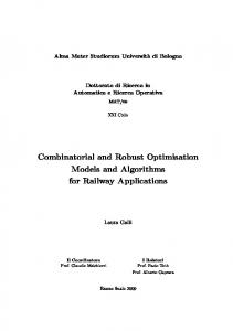
Figure 1 Quality-stability trade off in robust optimisation of a maximization problem.

ROBUSTNESS AND OPTIMISATION Many real-world optimisation problems are subject to uncertainties and noise. These uncertainties and noise are caused by manufacturing errors, measurement errors and external factors, e.g. the unpredictability of weather changes. The uncertainties emerge in different parts of the optimisation process. This makes it necessary to make a distinction between these different sources of uncertainties. Although manufacturing errors and measurements errors may be within an acceptable range, they can have a great influence on the characteristics of the building. Some minor deviations in the input variables of a system may result in great deviations in



Figure 1 illustrates an example of a simple onedimensional optimisation problem with the objective function f(x) and δ for uncertainties arising in design variables. This example is for a continuous function with one design variable, where the consideration of robustness leads to a different global optimum if a worst-case scenario is executed or performance fluctuation is fatal. If one is searching for the global optimum x1 is the preferred solution above x2, which forms a local optimum. However if the design variables x1 and x2 are subject to a deterministic quantified uncertainty this should have an effect on the function value of x1 much more than the function value of x2. Variable x2 has a nearly constant performance with respect to all possible variations around this variable. Variations around x1 on the other hand result in relatively higher performance drops and in the worst case the performance drops (at the first standard deviation) below the worst objective function value possible for x2. If guaranteed performance is required, one should select object x2. If instability of the objective function is not a problem, one can choose solutions for object x1. To understand the idea of a (partially) shifting Pareto front in robust optimisation, the example of a twodimensional minimization problem is given in Figure 2. Consider two design variables x1 and x2 and two objectives f1 and f2. The grey areas around the points in the x1 and x2 diagram represent the uncertainty of the design variables. Labels A and B connect the two objects with their corresponding objective function values. In this case, B has fewer declines regarding the average performance than A. If one thinks of an

imaginary Pareto front through the points (black dots) in the f1 and f2 diagram and thinks of another one though the worst-case points, one can see a shift in the direction of the upper right corner of the robust Pareto front. However, the domination of the two objects does not change in this case. Objective function vectors of the uncertainty sets A and B are mutually incomparable. It might be that a nondominated object in the Pareto front is dominated by another object in the robust Pareto front. In this case, this object is not of much interest anymore and is possibly replaced by a non-dominated solution.

  Figure 2 Quality-stability trade off in robust twodimensional optimisation. Figure 3 demonstrates the case. There is a considerable chance that either B or C gets dominated in the robust Pareto front. Two different main methods can be used to achieve robustness in the solutions (Deb & Gupta, 2006). The first method replaces the objective function with a mean effective function. Instead of choosing a best solution for the next generations an average solution is chosen. For this method it is required to have access to the objective function. The second method calculates a normalized difference between f and the perturbed function value fp.

Figure 3 Pareto front shift. In this paper a variant of the first method is proposed. Around a solution x 201 perturbations are generated. This number is based on Breesch (2004), who suggests that the number of simulations should be 1.5 times the number of input variables taken into consideration in order to achieve reliable results. The initial setup contains more than 130 parameters. The objective function value is obtained for each

perturbation and the worst solution, which is used to indicate a robust solution, is selected.

METAMODELS The meta-model or surrogate is a function of the design variables that approximates the objective function, thus, helping in fast assessing the robustness. Meta-models are built from the information gathered in previous evaluations of the objective functions. Meta-models are beneficial, because whenever applied they are much faster to evaluate than the original function. Some examples of techniques are, e.g., Kriging models (Kleijnen and Beers, 2004), neural networks (Badiru and Sieger, 1998), and response surface methodology (Ng et al., 2008). Kriging models in this research are used in conjunction with a sampler to generate an initial response surface. One issue of building performance simulation is the simulation time that increases whilst the amount of parameters gets higher and the results become more detailed. The motivation of using Kriging meta-models is to allow optimisation under uncertainty in a lower/ reduced time demand. Without meta-models the number of simulation runs in an optimisation is the number of optimizer iterations, the number of evaluations per iteration multiplied with the number of Latin hypercube samplings. With the use of Kriging meta-models the number of runs is reduced to the seeding runs and extra runs for online adaptation of the meta-model. In total, the number is reduced to a fraction of 5% to 20% of runs needed of the original algorithm. When an algorithm requires a large number of objective function calls to a computationally expensive function, this function can be partially replaced with a model used to compute the objective function faster, but approximated. For the problem in this work, where Monte Carlo sampling is used to allow robust optimisation and the objective function is computationally time expensive it is preferable and even necessary to partially replace evaluations with metamodels to achieve an acceptable runtime for the optimisations. Metamodels are an important class of surrogate models. They are based on the data of previous evaluations with the original model, which in most cases they interpolate. The model must be capable of spatial interpolation and is able to deal with multi-objective problems. Kriging (see also Figure 4) has its theoretical motivation in the theory of spatial random processes, so-called Gaussian random fields or briefly Gaussian processes. A Gaussian random field assigns a random variable Rx to each point in a d-dimensional Euclidean space. The random variables are normally distributed. A correlation between the random variables is given by a correlation function that depends on the distance; typical choices are the exponential correlation function, and the Gaussian correlation function. The estimation of the parameter

is done based on the given data maximum likelihood estimation.

Figure 4 Illustration of a Kriging metamodel of a one-dimensional objective function. The importance factor is a simple weight factor for each dimension in the search space. It is calculated as follows: for nf objectives and d design variables, take for each variable the minimum and maximum value in their range, while the remaining variables are attributed their mean values. For the variables xi with Gaussian distributed uncertainties the ranges are defined by their mean values E(xi) plus/minus three times the standard deviation S(xi). This covers at least 99% of the Gaussian distribution.

DESCRIPTION OF THE ALGORITHM As a multicriteria optimisation algorithm, we will use the SMS-EMOA (Beume et al. 2002). First, we will present it in its basic version, and second, we will introduce new features of the algorithm for finding robust solutions. The SMS-EMOA is based on the principle of hypervolume maximization. To understand this, let us first introduce the concept of the hypervolume measure as introduced by (Zitzler and Thiele, 1999) as a quality indicator for Pareto front approximations. Fleischer (2003) has shown that the maximization of the hypervolume measure leads to a set of points with each one of them positioned on the Pareto front. For discrete problems with a finite number of Pareto optima, he proved that the set that maximizes the hypervolume corresponds in the objective space with the Pareto front, given a sufficiently large reference point. While it is an open research question, how points distribute on higher dimensional Pareto front it has been found that they distribute in a favourable way in the 2-D case, provided the reference point coordinates are much larger than the highest values of the objective functions on the Pareto front (Auger et al. 2008). Hence, by maximizing the hypervolume of the objective function vectors of a set, a well

distributed approximation of the Pareto front can be achieved. This is the idea used in the SMS-EMOA. The basic loop of SMS-EMOA (Beume et al. 2002) looks as follows: The metamodel supported robust (¹ +1)-SMS-EMOA has to find robust solutions. As a robust fitness the worst sample out of 201 evaluations on the metamodel in a Monte Carlo simulation of the noise distribution is considered. An outline of the algorithm is given in the following: Algorithm: Metamodel-Assisted Robust SMSEMOA Input: problem dimension, variable bounds, objective functions Output: set of  solutions on (or close to) the Pareto front 1. Initialize population P(1) of  individuals. Each individual is a real-valued solution vector initialized randomly within the variable bounds. 2. Determine objective function vectors for all solutions in P(1) by evaluating  times black-box functions f1, …, fm and store all results in the archive A(1) 3. Set t = 1 4. Do until termination criterion fulfilled 4.1. Generate new child solution q(t) by applying recombination and random mutation operators based on the population P(t), evaluate its fitness f1, …, fm and store solution in archive 4.2. Determine the robust objective function vector for q(t) based on metamodel from archive 4.3. Select the set P(t+1) of  individuals from P(t) {q(t)} with maximal hypervolume measure of the corresponding objective function vectors 4.4. t=t+1 4.5. loop 5. Return P(t+1) Each parent is perturbed with a Monte Carlo sampling of 201 samples. For each perturbed point the objective function value is estimated with a metamodel. Non-dominated sorting is executed to partition the fronts in an increasing order. The worst front is the front that is dominated by all remaining fronts. For each point in the worst front the hypervolume contribution of this point is calculated. For the sample with the smallest hypervolume contribution the precise value is computed by the objective function. For the calculation of the correlation parameters a maximum likelihood heuristics is used. For the maximization of this likelihood term in Kriging meta-models a Covariance Matrix Adaptation Evolution Strategy (CMA-ES) is applied (Hansen et al., 2003). CMA-ES is a stochastic, population-based, iterative optimisation method belonging to the class

of evolutionary algorithms for continuous function optimisation.

CASE STUDY For the simulation we use a case study entitled “Het Bouwhuis” that is a building located in Zoetermeer, the Netherlands, between The Hague and Gouda, and is shown in Figure 5. It is the headquarters of Bouwend Nederland, the Dutch organisation of construction companies. The building is an ideal case study because it combines flexibility and function. Up to and including the detailed design phase, it was unclear whether to build option 1 (without double facade and cavity, less glazing and smaller office layout) or design option 2 as shown in Figure 6 and Figure 7. In both cases, the building has characteristics as follows.  Office building with 11 floors in a T-shaped plan.  Two levels/ stories underground parking (7000m²).  Flexible office concepts/ dispositions dividable from separate rooms up to open floor plan office solutions.

Figure 5 Illustration of ”Het Bouwhuis” 1.85m 12.00m 16.50m 0.85m

Figure 6 Illustration of the footprint for design option 2 of ”Het Bouwhuis”. In option 2, the building has a high percentage of glazing in the transparent facades: from the second floor up to the eleventh floor the building is on its “crosscut” sides provided with a double façade (see Figure 5 and Figure 6). The double skin is built one meter apart from the façade of the building; hence a magnifying cavity is created.

Figure 7 Illustration of the summer and winter case for design option 2 of ”Het Bouwhuis” (Nelissen, 2008). In winter, the ventilation air is drawn via the double skin façade where it is naturally pre-heated, then supplied as external air to the air handling unit. This method can be regarded as a heat-recovery system. In summer the double façade forms an extra barrier for solar radiation to enter the spaces as heat is removed from the façade air cavity through natural buoyancy driven ventilation to the outside. Another advantage is the increased noise barrier performance of the façade. The building is provided with a heat pump in combination with a heating-cooling storage. Both systems (summer and winter) are demonstrated in Figure 7. The double glass façade is designed to have a positive influence on energy savings and to provide superior comfort. For the assessment, the following characteristics are constituted:  Internal heat gains: equipments (20W/m²); people (10 W/m²) and lighting (15 W/m²).  Zoning: the assessment is conducted for the standard floor level comprising five zones (see Figure 6).  The assessment is based on the simulation of one room. All presented results relate to the smaller office room. The cavity space is located at the south- facing surface of the building (see Figure 6).  Set Points: The indoor set point in the office is 27°C for cooling and 21°C for heating. Table 1 Input parameters (maximum and minimum boundary conditions) for the optimisation with SMSEMOA algorithm. Min Glass area on two sides (m²)

Max 10

20

160

260

Internal gains: People (W/m²)

6

25

Internal gains: Lighting (W/m²) Internal gains: Equipment (W/m²)

6

35

6

30

Size room (m²)

To allow the optimisation under uncertainty, Kriging metamodels are used. Besides, the parameters varied for the optimisation, the distributions for uncertain parameters have to be defined. For the Kriging

metamodeling five variables for the optimisation shown in Table 1 (geometry room, window/ wall ratio, internal heat gains for people, equipment and lighting) and five variables for the uncertainty analysis (thickness wall layer, conductivity floor layer, infiltration rate, switch between double and single glazing) have been selected (cf Table 2). The optimisation parameters have been identified based on design team meetings by the project team and represent variations of the two different design options. The uncertainty parameters on the other hand have been identified in a pre conducteduncertainty and sensitivity study (cf. Hopfe and Hensen, 2011) where the five most sensitive ones have been selected. Table 2 Overview of Kriging meta-model input parameters for the optimisation and uncertainty analysis Thickness outside wall layer three t(m) μ 0.2 concrete block σ 0.02 Conductivity floor construction layer four λ(W/mK) μ 0.025 dense eps slab ins σ 0.00875 Conductivity roof construction layer two λ(W/mK) μ 0.5 felt/bitumen layer σ 0.25

algorithm. Important to note is the frequency of calls to the metamodel and the update of the metamodel with new points in the archive. To give an impression of the performance of the robust optimisation the following is carried out. From the initial population of a run with twenty parents a point is taken out. Around this point 50 perturbations (based on the decreased number of uncertain parameters) are randomly created and calculated by the objective function. The differences between the objective function values of the point and the objective function values of the perturbations is summed and divided by the number of perturbations. This results in an average deviation of the fifty calculated perturbations around the original point. This is repeated for all points in the populations. The same method is applied to all points in the final population after four hundred rounds of optimisation starting with the initial population. The initial population is shown as circles in the following Figures 9 -12, with the other dots indicating the different perturbations. For objective one (energy consumption), the solutions in the initial population show a better average robustness than the solutions in the final populations, in other words, the robustness has been declined. It is objective two (over- and underheating hours) that profits from the robust optimisation.

switch between double and single glazing Infiltration rate (ACH) between 0.5-1.0 The objective is to build a robust algorithm which finds a series of solutions for a two-objective minimization problem within a defined search space and within time constraints and where the objective function is a BPS tool (VA114) which acts as a black box. The Figure 8 presents a global overview of how the system will work.

Figure 8 System overview.

RESULTS Robust optimisation results for VA114 In Figure 9-12 are all optimisation results when using VA114 with a global metamodel supported

Figure 9 Scatter plot of the initial population (before optimisation) with its perturbations for a worst case scenario. Because the problem is two-dimensional it is the combination of the two objectives that is supposed to be robust. This is better explained with figures that show the objective functions values of the initial and final population together with the objective function values of the perturbations. Figure 9 involves the initial population and perturbations. The figure clearly shows the instability caused by the uncertainty in the design variables. It is not always the case that perturbed objection function values are worse compared to their original unperturbed objective function values, but it is impossible to guarantee the output values in a small range of the objective space. Figure 10 shows the

final population and their perturbations. This is certainly much more robust than it was in the initial situation.

robust optimisation. Again, the initial population and final population are given. Figure 12 clearly shows that after four hundred optimisation rounds the Pareto front is better than in the worst case, but with much more instability involved, caused by the uncertainty in the design variables.

CONCLUSION

Figure 10 Scatter plot of the final population (after optimisation) and its perturbations for a worst case scenario.

Figure 11 Scatter plot of the initial population (before optimisation) with its perturbations for a best case scenario.

Kriging metamodeling is an approach to reduce the number of objective function evaluations which becomes indispensable when the robustness of solutions needs to be tested in order to compare their performance. The results for the best, the mean, and the worst case give good insights to the behaviour of the objective function under consideration of only five variables for uncertainty. It is shown that it is possible to support a multiobjective algorithm with a metamodel and to optimize the problem to a robust Pareto front. Estimating the parameters of the metamodel with a maximum likelihood function does not result in the best possible result and slows down the optimisation. An importance factor makes a clear difference for the quality of the estimation of one of the objective function values. A local metamodel supported algorithm is working within the time constraint of one night of runtime. A disadvantage of Kriging is the limitation in the number of design variables (1-20) at which the metamodel still does quality estimations. This problem can be circumvented by reducing the number of parameters with the help of uncertainty and sensitivity analysis to identify the most sensitive variables. A local search method to fine tune the convergence to a local or global optimum is another task for the future. An idea is to compare a metamodel Assisted EA to an EA that uses parallel computing. With the increasing number of cores in processors these days, this is not that expensive anymore.

REFERENCES

Figure 12 Scatter plot of the final population (after optimisation) with its perturbations for a best case scenario. In the robust optimisation for this paper, a worst case scenario is chosen, that means that the worst solution out of 201 perturbations is compared with the current parent population. In Figure and Figure 12 it is demonstrated how a best scenario case performs in a

Auger, A., Bader, J., Brockhoff, D., Zitzler, E., 2008, Theory of the hypervolume indicator: optimal μ-distributions and the choice of the reference point, Proceedings of the tenth ACM SIGEVO workshop on Foundations of genetic algorithms, January 09-11, 2009, Orlando, Florida, USA Badiru, Adedeji B., and David B. Sieger. 1998. Neural network as a simulation metamodel in economic analysis of risky projects. European Journal of Operational Research 105, no. 1 (February 16): 130-142. El-Beltagy, M. A., Nair, P. B. and Keane, A. J., 1999. Metamodeling Techniques For Evolutionary Optimisation of Computationally Expensive Problems:

Promises and Limitations, Proceedings of the Genetic and Evolutionary Computation Conference, pp. 196-203, vol. 1 Beume, Nicola, Boris Naujoks, and Michael Emmerich. 2007. SMS-EMOA: Multiobjective selection based on dominated hypervolume. European Journal of Operational Research 181, no. 3 (September 16): 1653-1669. Breesch, H., and A. Janssens. 2004. Uncertainty and Sensitivity Analysis of the Performances of Natural Night Ventilation. In Proceedings of Roomvent 2004. Coimbra, Portugal.Deb, K. and Gupta, H., 2006. Introducing robustness in multi-objective optimisation. Evolutionary Computation, Vol. 14(4):463-494, December 2006. Emmerich, M.T.M., Hopfe, C.J., Marijt, R., Hensen, J.L.M., Struck, C. and Stoelinga, P., 2008. Evaluating optimisation methodologies for future integration in building performance tools. In Ian Parmee, editor, Proceedings of the 8th Int. Conf. on Adaptive Computing in Design and Manufacture (ACDM), 29 April - 1 May, Bristol, April 2008. Fleischer, M., 2003. The Measure of Pareto Optima Applications to Multi-objective Metaheuristics, C.M. Fonseca et al. (Eds.): EMO 2003, LNCS 2632, pp. 519–533, 2003. Springer, Heidelberg Hansen , N., S. D. Muller, and P. Koumoutsakos. 2003. Reducing the Time Complexity of the Derandomized Evolution Strategy with Covariance Matrix Adaptation (CMA-ES). Evolutionary Computation 11, no. 1: 1-18. Hopfe, C.J. & Hensen, J.L.M., 2011. Uncertainty analysis in building performance simulation for design support. Energy and Buildings, 43(10), pp.2798–2805. Hopfe, C.J., 2009. Uncertainty and sensitivity analysis in building performance simulation for decision support and design optimisation. PhD thesis, University of Eindhoven, Department of Building Engineering, 2009. Jin Yaochu, 2005: A comprehensive survey of fitness approximation in evolutionary computation. Soft Computing 9(1): 3-12 (2005) Kleijnen, J. P. C., and W. C. M. van Beers. 2004. Application-driven sequential designs for simulation experiments: Kriging metamodelling. Journal of the Operational Research Society 55, no. 8: 876–883.

Kruisselbrink, J.W. 2008. Robust optmization. March 17. Kruisselbrink, J.W., Emmerich, M.T.M, Baeck, T, 2010.: A Robust Optimisation Approach Using Kriging Metamodels for Robustness Approximation in the CMA-ES, IEEE Congress on Evolutionary Computation (CEC 2010), Barcelona, IEEE-Press, 2010. Magnier, L. & Haghighat, F., 2010. Multiobjective optimisation of building design using TRNSYS simulations, genetic algorithm, and Artificial Neural Network. Building and Environment, 45(3), pp.739–746. Marques, Michel, J.F. Pignatel, P. Saignes, F. D'Auria, L. Burgazzi, C. Muller, R. BoladoLavin, C. Kirchsteiger, V. La Lumia, and I. Ivanov. 2005. Methodology for the reliability evaluation of a passive system and its integration into a Probabilistic Safety Assessment. Nuclear Engineering and Design 235, no. 24 (December): 2612-2631. Ng, K.C., K. Kadirgama, and E.Y.K. Ng. 2008. Response surface models for CFD predictions of air diffusion performance index in a displacement ventilated office. Energy and Buildings 40, no. 5: 774-781. Sacks, J., Welch, W. J., Mitchell, W. J. and Wynn, H.-P. 1989. Design and analysis of computer experiments. Statistical Science, 4(4):409-435, 1989. Schueller, G.I., and H.A. Jensen. 2008. Computational methods in optimisation considering uncertainties - An overview. Computer Methods in Applied Mechanics and Engineering 198, no. 1 (November 15): 2-13. Taguchi, G. 1989. Introduction to Quality Engineering. American Supplier Institute. VABI. Handleiding, 2009. http://www.vabi.nl/downloads/. Wright, J., Zhang, Y., Angelov, P.P. and Buswell, R.A.. Building system design synthesis and optimisation. In Final Report to ASHRAE on Research Project 1049-RP, 2004. Zitzler, E. and Thiele, L., 1998. Multiobjective optimisation using evolutionary algorithms a comparative case study. In A. E. Eiben et al, editor, Parallel Problem Solving from Nature - PPSN V, Amsterdam, pages 292301, Berlin, 1998. Springer.