Robust numerical methods for robust control Peter Benner∗∗‡
Ralph Byers§¶
Volker Mehrmann††‡
Hongguo Xu§k April 14, 2004
Abstract We present numerical methods for the solution of the optimal H∞ control problem. In particular, we investigate the iterative part often called the γ-iteration. We derive a method with better robustness in the presence of rounding errors than other existing methods. It remains robust in the presence of rounding errors even as γ approaches its optimal value. For the computation of a suboptimal controller, we avoid solving algebraic Riccati equations with their problematic matrix inverses and matrix products by adapting recently suggested methods for the computation of deflating subspaces of skew-Hamiltonian/Hamiltonian pencils. These methods are applicable even if the pencil has eigenvalues on the imaginary axis. We compare the new method with older methods and present several examples.
Keywords. H∞ control, algebraic Riccati equation, CS decomposition, Lagrangian subspaces, skew-Hamiltonian/Hamiltonian pencil, AMS subject classification. 93B40, 93B36, 65F15, 93B52, 93C05. ∗∗
Fakult¨ at f¨ ur Mathematik, TU Chemnitz, D-09107 Chemnitz, FRG;
[email protected] § Department of Mathematics, University of Kansas, Lawrence, Kansas, USA; {byers,xu}@math.ukans.edu. †† Institut f¨ ur Mathematik, TU Berlin, Straße des 17. Juni 136, D-10623 Berlin, FRG;
[email protected]. ¶ This author was partially supported by National Science Foundation grants 0098150, 0112375, and 9977352. k This author was partially supported by National Science Foundation grant 0314427, and the University of Kansas General Research Fund allocation # 2301717. ‡ These authors were partially supported by Deutsche Forschungsgemeinschaft, Research Grants Me 790/11-3, Bu 687/12-1, Be 2174/4-1, and the DFG Research Center “Mathematics for Key Technologies” (FZT86) in Berlin.
1
1
Introduction
The optimal infinite-horizon output (or measurement) feedback H∞ control problem is one of the central tasks in robust control, see, e.g., [20, 30, 38, 41], but the development of robust numerical methods for the H∞ control is unusually difficult [37] and remains a major open problem [12]. This paper derives a numerical method with better robustness in the presence of rounding errors than other methods. The H∞ norm of a matrix valued rational function F (s) that is analytic and bounded in the open right-half plane is kF k∞ = supω∈R σmax [F (iω)], where σmax [F (iω)] denotes the maximal singular value of the matrix F (iω). In robust control, the H∞ norm of a transfer function from disturbance inputs to error outputs is a measure of the worst case influence of disturbances. The optimal H∞ control problem is the task of designing a dynamic controller that minimizes this measure. Consider the linear system x˙ = Ax + B1 w + B2 u,
x(t0 ) = x0 ,
z = C1 x + D11 w + D12 u,
(1)
y = C2 x + D21 w + D22 u, where A ∈ Rn,n , Bi ∈ Rn,mi , Ci ∈ Rpi ,n , and Dij ∈ Rpi ,mj for i, j = 1, 2. (By Rn,k we denote the set of real n × k matrices.) As usual, see [20, 41], we assume p1 ≥ m2 and m1 ≥ p2 . In this system, x(t) ∈ Rn is the state vector, u(t) ∈ Rm2 is the control input vector, and w(t) ∈ Rm1 is an exogenous input that may include noise, linearization errors and unmodeled dynamics. The vector y(t) ∈ Rp2 contains measured outputs, while z(t) ∈ Rp1 is a regulated output or an estimation error. Definition 1.1 The Optimal H∞ control problem: Determine a controller (dynamic compensator) ˆx + By, ˆ x ˆ˙ = Aˆ ˆ ˆ u = Cx ˆ + Dy,
(2)
ˆ ∈ Rm2 ,p2 and transfer function ˆ ∈ RN,p2 , Cˆ ∈ Rm2 ,N , D with Aˆ ∈ RN,N , B −1 ˆ ˆ ˆ ˆ K(s) = C(sI − A) B + D such that the closed-loop system resulting from (1) and (2), ˆ 1 C2 )x + (B2 Z2 C)ˆ ˆ x + (B1 + B2 DZ ˆ 1 D21 )w, x˙ = (A + B2 DZ ˆ 1 D22 C)ˆ ˆ 1 C2 x + (Aˆ + BZ ˆ x + BZ ˆ 1 D21 w, x ˆ˙ = BZ ˆ 2 )x + D12 Z2 Cˆ x ˆ 1 D21 )w, z = (C1 + D12 Z2 DC ˆ + (D11 + D12 DZ 2
(3)
ˆ −1 and Z2 = (I − DD ˆ 22 )−1 , is internally stable, (i.e., with Z1 = (I − D22 D) the solution of the system with w ≡ 0 is asymptotically stable), and the closed-loop transfer function Tzw (s) from w to z is minimized in the H∞ norm. The solution of the problem is, in general, difficult. Solving the H∞ control problem by directly minimizing kTzw k∞ over the complicated set of internally stabilizing controllers (2) is intractable by conventional optimization methods. It is often unclear whether a minimizing controller exists [41, p.414]. When a minimizing controller or an approximately minimizing controller does exist, it is typically not unique. Nevertheless, the well-known state-space solution to the H∞ control problem [15], relating H∞ control to algebraic Riccati equations, provides a way to solve many H∞ control problems despite the above difficulties. We review this solution as presented in [41] as Theorem 3.5 in Section 3. However, in summary, for each number γ > 0, the theorem gives an explicit computational test the existence of an internally stabilizing dynamic controller (3) whose closed-loop transfer function Tzw (s) satisfies γ > kTzw k∞ . Explicit but complicated formulas in terms of γ for a dynamic controller that achieves γ > kTzw k∞ (when one exists) appear, e.g., in [21, 41] and are discussed in [6]. Hence, at least in principle, the theorem can be used to solve the H∞ control problem by bisection on γ. Here, we view the theorem as a tool to divide the optimal H∞ problem into two subproblems that we call the modified optimal H∞ control problem and the suboptimal H∞ control problem. Definition 1.2 The Modified optimal H∞ control problem: Let Γ be the set of numbers γ > 0 for which there exists an internally stabilizing dynamic controller with transfer function Tzw (s) satisfying γ > kTzw k∞ . Determine γmo = inf Γ. (If no internally stabilizing controller exists, then Γ = ∅ and γmo = ∞.) The modified optimal H∞ control problem is an optimization in the single independent variable γ, while the optimal H∞ control problem requires optimization over the complicated set of stabilizing controllers. Because it may be impractical or unnecessary to determine γmo to high precision and because there may be no dynamic controller whose transfer function actually achieves H∞ norm equal to γmo , in general, is is necessary to use a controller whose transfer function has larger H∞ norm, i.e., a suboptimal controller.
3
Definition 1.3 The Suboptimal H∞ control problem: For a given value γ ∈ Γ, find an internally stabilizing dynamic controller such that the closed loop transfer function satisfies kTzw k∞ < γ. The process of solving the modified optimal H∞ control problem is sometimes called the γ-iteration. Once a sufficiently accurate approximation to γmo has been determined, a suboptimal controller may be constructed using the formulas suggested in [21, 41] or by the more robust formula in [6]. In this paper we present rounding-error robust numerical methods for the γ-iteration. The modified optimal H∞ control problem is well analyzed, [20, 30, 38, 41] and numerical methods have been implemented in several software packages [7, 18, 13, 31]. The accuracy of conventional methods like these is limited by the empirical fact that as γ approaches γmo , the Riccati equations and other subproblems tend to become so ill-conditioned that rounding errors make it impossible to use the test in Theorem 3.5. The procedures may fail before an accurate approximation of γmo is obtained. This paper presents numerical methods that (mostly) overcome this problem.
2
Preliminaries
In this section we introduce some notation and definitions. By Rn,k we denote the set of real n × k matrices. For symmetric matrices A and B, A ≥ B and A > B mean that A − B is positive semidefinite and positive definite, respectively. By A† ∈ Rk,n we denote the Moore-Penrose inverse of the matrix A ∈ Rn,k . An eigenvalue λ of a square matrix A is stable (semi-stable) if its real part is negative (zero). A square matrix A is stable (semi-stable) if all the eigenvalues of A are in the open (closed) left half complex plane. i h Definition 2.1 Let J := −I0 n I0n , where In is the n × n identity matrix. a) A matrix H ∈ R2n,2n is Hamiltonian if (HJ )T = HJ and H ∈ R2n,2n is skew-Hamiltonian if (HJ )T = −HJ .
b) A matrix Z ∈ R2n,2n is symplectic if ZJ Z T = J and U ∈ R2n,2n is orthogonal symplectic if UJ U T = J and U T U = I2n . c) An invariant subspace L of a Hamiltonian matrix H ∈ R2n,2n is Lagrangian if it is n-dimensional and xH Jy = 0, for all x, y ∈ L. 4
d) An invariant subspace L of a Hamiltonian matrix H ∈ R2n,2n is stable (semi-stable) Lagrangian if it is Lagrangian and corresponds to the eigenvalues of H in the open (closed) left half complex plane. Real Hamiltonian matrices take the form ¸ · F −G , H= −K −F T
(4)
where F, G, K ∈ Rn,k , G = GT and K = K T . To each Hamiltonian matrix there corresponds an algebraic Riccati equation F T X + XF + K − XGX = 0,
(5)
which is often encountered in control design. Definition 2.2 A matrix X is a stabilizing (semi-stabilizing) solution of (5) if X = X T and F − GX is stable (semi-stable). It is well known [23, 27] and easy to verify that if X is a stabilizing (semistabilizing) solution of the algebraic Riccati equation (5), then the columns h i In of X span a stable (semi-stable) Lagrangian invariant subspace of the h i 1 Hamiltonian matrix (4). Conversely, if the columns of X X2 span a stable (semi-stable) Lagrangian invariant subspace of the Hamiltonian matrix (4) and X1 is nonsingular, then X = X2 X1−1 is a stabilizing (semi-stabilizing) solution of the algebraic Riccati equation (5). Example 2.3 The one-dimensional algebraic Riccati equation 0x2 + 2x + 1 = 0 has no positive solution, but the corresponding Hamili h semidefinite 1 0 tonian matrix H = 1 −1 has the unique Lagrangian invariant subspace £ ¤ L = span 01 , corresponding to the eigenvalue −1. In this example K = [1], F = [1] and G = [0], so the pair (K, G) is not stabilizable. Example 2.4 The one dimensional algebraic Riccati equation x2 +3x+2 = 0 has no positive semidefinite solution, but its corresponding Hamiltonian h i 1.5 −1 matrix H = 2 −1.5 has the unique Lagrangian invariant subspace L = £1¤ 2 corresponding to the eigenvalue −1/2. In this example G = [−1] which is not positive semidefinite. Conventional numerical methods for the modified optimal H∞ control problem require the computation of the stabilizing solution of Riccati equations of the form (5) in which F and/or G are not necessarily semidefinite 5
or for which (K, F ) is not stabilizable or (K, G) is not detectable. Such algebraic Riccati equations may have no positive semidefinite semi-stabilizing solution [23, 27]. This is one source of trouble in numerical methods for the modified optimal H∞ control problem. This paper presents a numerical method that circumvents this problem by working directly with the semi-stabilizing Lagrangian subspace.
3
Theoretical Background
In this section we discuss the theoretical background for the modified optimal H∞ problem. We start with a typical set of assumptions [21, 20, 30, 41]. Assumptions: A1. The pair (A, B2 ) is stabilizable and the pair (A, C2 ) is detectable. A2. D22 = 0 and both D12 and D21 have full rank. h i B2 A3. The matrix A−iωI C1 D12 has full column rank for all real ω. h i B1 A4. The matrix A−iωI C2 D21 has full row rank for all real ω.
Remark 3.1 The requirement that D22 = 0 (Assumption A2) is for convenience. Systems that have a direct link from input to output, i.e., for which D22 6= 0, can be synthesized by first studying the problem without this term, see [41]. h i In the literature, it is often assumed that D12 = Im0 and D21 = [0, Ip2 ] 2 and that D11 = 0. In principle, this particular form can be obtained from a more general system by transforming the system in advance. Unfortunately, reducing the system to this form may require ill-conditioned transformations that lead to unnecessary numerical errors. We allow general D12 , D21 and D11 subject to Assumption A2. (Note that this leads to slightly different solution formulas for the optimal feedbacks and the closed-loop system than those given in [21, 41]. See [6] for more general and numerically more robust formulas.) To formulate the basic theorem of H∞ control, we introduce the following two symmetric matrices depending on the Dij and a parameter γ ∈ R, ¸ · 2 · T ¸ ¤ γ Im1 0 D11 £ D11 D12 − , RH (γ) := T 0¸ · D12 ¸ · 20 (6) ¤ D11 £ T γ Ip1 0 T D11 D21 RJ (γ) := − . D21 0 0 6
Conventional H∞ numerical methods require that both RH (γ) and RJ (γ) are nonsingular. The following proposition provides a convenient test. Proposition 3.2 If Assumption A2 is not satisfied, then either RH is singular for all γ or RJ is singular for all γ. If Assumption A2 holds, then there exist only a finite number of values of γ ≥ 0 for which one or both of the matrices RH (γ) or RJ (γ) is singular. Definition 3.3 Define γˆH , γˆJ and γˆ by γˆH := max{γ ∈ R | RH (γ) is singular }, γˆJ := max{γ ∈ R | RJ (γ) is singular } and γˆ := max{ˆ γH , γˆJ }. If D11 = 0, then hγˆ = i0. If D11 6= 0, then γˆ is typically positive. T and D T Let D12 = U12 Σ012 V12 21 = V21 [0, Σ21 ]U21 be (slightly permuted) singular value decompositions of D12 and D21 with real orthogonal matrices U12 , U21 , V12 , V21 and nonnegative diagonal matrices Σ12 and Σ21 . Use the orthogonal equivalence transformation ¸ ¸· ¸· · T D1 D2 0 D11 D12 U21 0 U12 0 = D3 D4 Σ12 T 0 V21 D21 0 0 V12 0 Σ21 0 to define D1 , D2 , D3 and D4 .
Proposition h 3.4 i [41] If Assumption A2 holds, then γˆH = σmax [D1 , D2 ], D1 γˆJ = σmax D3 and the following equivalences hold. i) RH (γ) is invertible if and only if D1 D1T + D2 D2T − γ 2 I is invertible.
ii) RJ (γ) is invertible if and only if D1T D1 + D3T D3 − γ 2 I is invertible. The next theorem gives the theoretical basis for the γ-iteration. Theorem 3.5 [41]. Consider system (1), with RH and RJ as in (6). Under assumptions A1–A4, there exists an internally stabilizing controller such that the transfer function from w to z, Tzw , satisfies kTzw k∞ < γ if and only if the following four conditions hold. 1. γ > γˆ with γˆ as in Definition 3.3. 2. There exists a stabilizing positive semidefinite solution XH = XH (γ) of the algebraic Riccati equation associated with the Hamiltonian matrix ¸ · A 0 −1 T − BH RH (γ)BH J, (7) H(γ) = −C1T C1 −AT i h where BH = −CBT 1D11 −CBT 2D12 . 1
1
7
3. There exists a stabilizing positive semidefinite solution XJ = XJ (γ) of the algebraic Riccati equation associated with the Hamiltonian matrix · ¸ AT 0 J(γ) = − J CJT RJ−1 (γ)CJ , (8) −B1 B1T −A where CJ :=
h
D11 B1T C1 D21 B1T C2
i .
4. γ 2 > ρ(XH XJ ). (Here ρ(XH XJ ) denotes the spectral radius of XH XJ .) The solution to the suboptimal control problem, γmo , is the supremum of all γ ≥ 0 for which at least one of the conditions in Theorem 3.5 fails.
4
Conventional Numerical Methods
This section discusses finite precision arithmetic hazards encountered by typical numerical methods for checking the four conditions in Theorem 3.5. Finite precision hazards are also discussed in [17, 21, 37]. Conventional numerical methods for the solution of the modified optimal H∞ problem [31, 37] fall into two categories. The first embeds the problem into a linear matrix inequality [10] and employs methods of semidefinite programming to find γmo . This is attractive, because easy-to-use methods for semidefinite programming are available, see, e.g., [18, 28]. However, O(n6 ) computational complexity grows so rapidly that these methods are practical only for low-dimensional problems. The second is the category of Riccati methods. A typical Riccati method uses Theorem 3.5 to find upper and lower bounds on γmo which are then refined by bisection also using Theorem 3.5. A quadratically convergent method based on Newton’s method can be found in [34]. Each iterative step includes checking whether γ > γˆ , using a Riccati solver like those discussed in [2, 3, 27, 35] to compute stabilizing solutions XH and XJ (if they exist) corresponding to (7) and (8), and then checking whether γ 2 > ρ(XH XJ ). This approach has complexity O(n3 ) per step and is currently the only practical choice for higher dimensional problems. Unfortunately there are several numerical difficulties associated with the Riccati method. Primary among these is the fact that often as γ approaches γmo , one of the Riccati solutions XH or XJ either diverges to ∞ or becomes highly ill-conditioned, i.e., tiny errors in the Hamiltonian matrices H(γ) or J(γ) may lead to large errors in XH or XJ . The following example, which we will use frequently, demonstrates. 8
Example 4.1 Consider the system
A B1 B2 C1 D11 D12 = C2 D21 0
−1 0 ǫ1 0 −1 0 α 0 12 0 β 0 δ η 0
If ǫ1 = ǫ2 = 0, then (6) becomes
RH (γ) = RJ (γ) =
1 4
− γ2 0 0
1 4
0 − γ2 1 2
0 1 ǫ2 1 0 0 . 1 1 2 1 0 0 1 2
1
,
and γˆ = 21 . With ζ(γ) := 1 − 41 γ −2 , the Hamiltonian matrices (7) and (8) become −1 −β −ζ(γ) −ζ(γ) 0 −1 − β −ζ(γ) −ζ(γ) H(γ) = α2 − 1 0 0 ζ(γ) 0 0 β 1+β and
−2 − δηζ(γ) − βδ −1 0 α2 γ −2 ζ −1 (γ) − δ 2 ζ(γ) 2 γ −2 − δηζ(γ) 0 −1 − βδ (β − η)βγ −2 − η 2 ζ(γ) . 2 γ J(γ) = 0 0 1 0 0 0 0 1
The matrix J(γ) has the double stable eigenvalue −1 and the corresponding positive semidefinite p Riccati solution is XJ = 0. The matrix H(γ) has two eigenvalues −1, − (1 + β)2 p + α2 in the open left half complex plane. 1 When γ > 2 , setting ν := 1 + (1 + β)2 + α2 , the positive semidefinite Riccati solution corresponding to H(γ) is " ¡ ¢ # 2 β(2+β) + αν β(2³+ β) ν1 − 21´ α2 2 ¢ ¡ · . XH = (2+β) ζ(γ)(2β + β 2 + α2 ) β 2 21 − ν(ν+β) β(2 + β) ν1 − 12 (If β 2 + 2β + α2 = 0, then XH
α2 = 8ζ(γ)
"
4 − α2 α2
9
2 ´ ³ α 2 β 2 1 + 2+β
#
.
√ Note in this case |α| ≤ 1 and β = −1 ± 1 − α2 . Moreover, H(γ) has the double eigenvalues 1 and −1.) Since the semi-stabilizing Riccati solutions XH and XJ exist and ρ(XJ XH ) = 0 for all γ > γˆ , we have γmo = γˆ = 21 . As γ approaches γmo , ζ(γ) approaches 0. RH and RJ become singular, the Hamiltonian matrices H(γ) and J(γ) become ill-defined, and the Riccati solution XH converges to infinity. Typical numerical Riccati solvers are unable to succeed on problems as extreme as those in Example 4.1 with γ ≈ γˆ . Failing to solve a Riccati equation may cause a computation to abort before attaining a close approximation to γmo [21]. In the most extreme case, H(γ), J(γ) or a Riccati solution may have entries larger than the overflow threshold and not be representable in the working floating point number system, thus guaranteeing failure of any numerical method that explicitly constructs any of the matrices in Theorem 3.5! A more subtle and more likely problem (also observed in [17]) is that explicitly forming the Hamiltonian matrices themselves may lead to large inaccuracies. If the matrices RH (γ) or RJ (γ) are ill-conditioned or if cancellation errors occur in computing the blocks of H(γ) and J(γ), then the input data for the Riccati solvers may be corrupted. Example 4.1 demonstrates how the matrices RH (γ) and RJ (γ) become nearly singular and highly illconditioned as γ approaches γˆ = γmo . To facilitate our discussion, we need notation for several critical points of γ that play roles determining γmo . R, γ Definition 4.2 Define γˆH ˆJR and γˆ R as ¯ ¯ The Riccati equation corresponding to H(γ) ¯ R γˆH = inf γ ≥ γˆ ¯¯ in (7) has a positive semi-definite, semi- , ¯ stabilizing solution. ¯ ¯ The Riccati equation corresponding to J(γ) ¯ γˆJR = inf γ ≥ γˆ ¯¯ in (8) has a positive semi-definite, semi- , ¯ stabilizing solution. R γˆ R = max(ˆ γH , γˆJR ).
L, γ Definition 4.3 Define γˆH ˆJL and γˆ L as ¯ ¾ ½ ¯ The Hamiltonian matrix H(γ) in (7) has a L ¯ , γˆH = inf γ ≥ γˆ ¯ semi-stable Lagrangian invariant subspace. ¯ ¾ ½ ¯ The Hamiltonian matrix J(γ) in (8) has a , γˆJL = inf γ ≥ γˆ ¯¯ semi-stable Lagrangian invariant subspace. L γˆ L = max(ˆ γH , γˆJL ).
10
I , γ Definition 4.4 Define γˆH ˆJI and γˆ I as ¯ ½ ¯ The Hamiltonian I γˆH = sup γ > γˆ ¯¯ eigenvalue on the ¯ ½ ¯ The Hamiltonian γˆJI = sup γ > γˆ ¯¯ eigenvalue on the
γˆ I
I = max(ˆ γH , γˆJI ).
matrix H(γ) in (7) has an imaginary axis. matrix J(γ) in (8) has an imaginary axis.
¾
¾
, ,
If both H(γ), J(γ) have no eigenvalues on the imaginary axis for all γ > γˆ , γˆ I does not exist. If γ = γˆ I , then one or both of the Hamiltonian matrices H(γ) or J(γ) have eigenvalues on the imaginary axis. Even with otherwise robust numerical methods like the QR algorithm, rounding errors made while calculating eigenvalues and invariant subspaces may introduce non-Hamiltonian perturbations of the Hamiltonian matrix. Unstructured, non-Hamiltonian rounding errors may destroy the uniqueness of the semi-stable Lagrangian invariant subspace [32, 33] causing a Riccati solver to fail. Even the number of eigenvalues in the closed left-half plane may drop below its theoretical minimum of n. The following example illustrates this effect. (See also Section 7.) Example 4.5 Consider the Hamiltonian matrix with non-Hamiltonian perturbation −2 1 1 0 ε 0 0 0 −4 2 0 1 + ε ε 0 0 , H(ε) := H + E := 0 0 2 4 0 0 ε ε 0 0 −1 −2 0 0 0 ε
The unperturbed matrix (ε = 0) has eigenvalue λ = 0 with algebraic multiplicity 4 and geometric multiplicity 1. There is a unique, Lagrangian semistable, two-dimensional invariant subspace which is spanned by the first two columns of the identity matrix. √ √ The perturbed matrix (ε 6= 0) has eigenvalues ε ± ε and ε ± −ε. The symmetry in the spectrum is lost. If −1 < ε < 0, then three eigenvalues lie in the open left-half plane and there are three two-dimensional stable invariant subspaces. (Despite the non-Hamiltonian perturbation, one of the two-dimensional stabilizing invariant subspaces is Lagrangian.) If 1 > ε > 0, then only one eigenvalue lies in the open left-half plane and there is no twodimensional stable invariant subspace. 11
Many Riccati equation solvers begin their work by extracting the stable invariant subspace of a Hamiltonian matrix [3, 24, 27, 35]. A naive algorithm applied to this Hamiltonian matrix may select an incorrect invariant subspace and either conclude that there is no solution to the Riccati equation or simply return a far-from-symmetric and/or non-stabilizing solution. Note that the signs of the real parts of eigenvalues are of little help in determining which of the two-dimensional invariant subspaces might be used—even when ε = 0! The unperturbed Hamiltonian matrix has a quadruple eigenvalue; the loss of the eigensymmetry in the perturbed matrix obscures the semi-stable Lagrangian invariant subspace. The eigenvalues of real Hamiltonian matrices are symmetric about both the real axis and the imaginary axis, see [23, 25, 27]. Eigenvalues with nonzero real and imaginary parts occur in quadruples consisting of two ± ¯ −λ. ¯ Real eigenvalues and pure imaginary eigenvalues appear pairs, λ, −λ, λ, in ± pairs. A Hamiltonian perturbation of H in Example 4.5 could not create confusion, because the ± pairing of eigenvalues would be preserved. A numerically stable algorithm that fully exploits Hamiltonian structure would introduce Hamiltonian-structured rounding errors and avoid some of the discussed numerical difficulties. The design of such a method is a difficult problem which is still partially unsolved. But recent progress has lead to new methods [1, 5, 8, 9] that are almost ideal in the sense that they are numerically stable and exploit the structure of the Hamiltonian matrices to a very large extent. Example 4.6 Consider Example 4.1 with α = β = δ = η = ǫ2 = 1 and ǫ1 = 0. In this case, the Riccati solution associated with (8) has semi-stabilizing solution XJ = 0, independent of γ. We constructed H(γ) in (7) for 91 values of γ equally spaced in the interval [0.1, 1] and used the Matlab builtin function eig (based on the QR algorithm, see, e.g., [19]) to calculate the eigenvalues of each H(γ). In no case did any computed eigenvalue have zero real part. If a Hamiltonian matrix has no eigenvalue with zero real part, then there is a unique stabilizing solution of the corresponding algebraic Riccati equation. A naive program to calculate γmo might use this to conclude that the algebraic Riccati equation corresponding to each H(γ) has a stabilizing solution for γ ∈ [.5, 1]. Such a program might even construct “solutions” XH , calculate ρ(XH XJ ) = 0 and ultimately conclude that γmo = γˆ = 1/2. In fact, γmo = γˆ I ≈ 0.806. In this example, the algebraic Riccati equation corresponding to (7) has a stabilizing positive semidefinite solution if 12
and only if γ > γˆ I . As γ approaches γˆ I , a ±λ pair of real eigenvalues of the Hamiltonian matrix H(γ) in (7) coalesces into a double eigenvalue at 0 corresponding to a 2-by-2 Jordan block. As γ decreases further, this double eigenvalue splits into two complex conjugate eigenvalues with zero real part. Rounding errors constructing H(γ) and computing its eigenvalues perturb eigenvalues off the imaginary axis. If these rounding errors are of magnitude ε then the eigenvalues of the 2-by-2 Jordan block are perturbed √ by O( ε). Similar eigenvalue perturbations result from perturbations of γ near γˆ I . Thus, eigenvalues may be relatively distant from the imaginary axis even when γˆ ≈ γˆ I . Consequently, it is problematical to use the computed eigenvalues to determine whether H(γ) has eigenvalues with zero real part and whether the corresponding algebraic Riccati equation has a stabilizing solution. Definition 4.7 Let XH = XH (γ), XJ = XJ (γ) be the positive semidefinite stabilizing solutions of the Riccati equations associated with H(λ) and J(λ) in Theorem 3.5, respectively. Define γˆ ρ to the largest number γ ≥ γˆ satisfying γ 2 = ρ(XH XJ ). If no such number γ exists, then γˆ ρ does not exist. Under Assumptions A1-A4, γˆ , γˆ L and γˆ R satisfy 0 ≤ γˆ ≤ γˆ L ≤ γˆ R . If γˆ I exists, then γˆ I = γˆ L > γˆ . If γˆ ρ exists, then γˆ ρ ≥ γˆ R . Note that γmo = max(ˆ γ , γˆ L , γˆ R , γˆ ρ ).
5
Reformulations
The following section reviews the properties of Lagrangian invariant subspaces and Riccati solutions associated with H(γ) and J(γ) along with the relationship between γmo and the various γˆ ’s. This section also reformulates Theorem 3.5 in order to overcome numerical difficulties.
5.1
Avoiding explicit solution of Riccati equations
The solution of the algebraic Riccati equations is only an intermediate step toward solving the H∞ control problem. Avoiding explicit solution of algebraic Riccati equations is the only way to avoid numerical instabilities like those in Example 4.1. A similar situation occurs in H2 control problems. There, the solution of algebraic Riccati equations is an intermediate step toward the closed-loop matrix and optimal feedback. Explicit Riccati solutions may be avoided by computing deflating subspaces of matrix pencils [4, 5, 39]. 13
A reformulation of Theorem 3.5 suggested in [41, Theorem 16.4, p. 419] employs this idea. Conditions 2 and 3 in Theorem 3.5 may be replaced by the following alternative conditions. 2’. There exist matriceshXH,1i, XH,2 ∈ Rn,n with XH,1 nonsingular such XH,1 that the columns of X , span a semi-stable Lagrangian invariant H,2 subspace of H(γ), i.e., there exists a semi-stable matrix TH for which · ¸ · ¸ XH,1 XH,1 H(γ) = TH . (9) XH,2 XH,2 n,n with X 3’. There exist matrices X J,1 nonsingular such that h i J,1 , XJ,2 ∈ R XJ,1 the columns of XJ,2 , span a semi-stable Lagrangian invariant subspace of J(γ), i.e., there exists a semi-stable matrix TJ for which · ¸ · ¸ XJ,1 XJ,1 J(γ) = TJ . (10) XJ,2 XJ,2
(Below, we further reformulate the invariant subspace approach and remove the non-singularity requirement for XH,1 and XJ,1 .) I (or γ = γ The reformulation is helpful, because when γ = γˆH ˆJI ), then H(γ) (or J(γ)) may have a unique semi-stable Lagrangian subspace but no positive semi-stabilizing solution to the associated Riccati equation. Furthermore, there exist Hamiltonian matrices for which the computation of the unique semi-stable Lagrangian invariant subspace is well-conditioned, but the solution of the Riccati equation is ill-conditioned.
5.2
Avoiding the spectral radius condition
In order to avoid explicit Riccati solutions entirely, we must also reformulate Condition 4 of Theorem 3.5, ρ(XH XJ ) < γ 2 , in terms of the invariant semi-stable, Lagrangian invariant subspaces (9) and (10). (See also [41, Section 16.11].) Fori this hpurpose,i we introduce the following symmetric h XH,1 (γ) XJ,1 (γ) matrix. Let X (γ) and X be as in (9) and (10), respectively. Set (γ) H,2
J,2
Y(γ) :=
·
T X T X γXH,2 XH,2 H,1 J,2 T T X XJ,2 XH,2 γXJ,2 J,1
¸
.
(11)
Note that all the blocks of Y are functions of γ, even if γ does not appear explicitly in the off-diagonal blocks. If there is no semi-stable, Lagrangian 14
invariant subspace, then Y(γ) is undefined. We will show that Y(γ) is positive semidefinite with a particular rank if and only if the Riccati solutions XH and XJ in Theorem 3.5 exist and γ 2 > ρ(XH XJ ). First recall that the ranks of XH = XH (γ) and XJ = XJ (γ) are constant for γ > γmo . Theorem 5.1 [15, 22, 40] Under assumptions A1-A4, γmo exists. The solutions XH = XH (γ) and XJ = XJ (γ) of the algebraic Riccati equations associated with H(γ) and J(γ) in (7) and (8) as well as the spectral radius ρ(XH XJ ) = ρ(XH (γ)XJ (γ)) are monotone decreasing functions of γ on the infinite interval I = (γmo , ∞), i.e., if γmo < γ1 ≤ γ2 , then XH (γ2 ) ≤ XH (γ1 ), XJ (γ2 ) ≤ XJ (γ1 ) and ρ(XH (γ2 )XJ (γ2 )) ≤ ρ(XH (γ1 )XJ (γ1 )). In addition, the ranks of XH = XH (γ) and XJ = XJ (γ) are constant on I. Proof. See [15, 40]. For particularly complete proofs, see [22, Theorems 2.4, 4.1, 5.1]. The following well-known theorem on the CS decomposition of orthonormal bases of Lagrangian subspaces helps display the internal structure of Y(γ). h i 1 Lemma 5.2 [29] If X1 , X2 ∈ Rn,n and the columns of X X2 form an orthonormal basis of a Lagrangian subspace, then there exist orthogonal matrices U ∈ Rn,n and V ∈ Rn,n such that U T X1 V = C and U T X2 V = S are both diagonal and C 2 + S 2 = I. h i h i XJ,1 (γ) H,1 (γ) Apply Lemma 5.2 to X , separating diagonal elements of C XH,2 (γ) XJ,2 (γ) and S that equal zero or one to get
T XH,1 VH = CH UH
T UH XH,2 VH = SH
UJT XJ,1 VJ = CJ
=:
=:
=:
rH kH n − tH rH kH n − tH
rH 0 0 0
rH I 0 0
rJ rJ 0 0 kJ n − tJ 0
15
kH 0 ΣH 0 kH 0 ∆H 0 kJ 0 ΣJ 0
n − tH 0 0 , I
n − tH 0 0 , 0
n − tJ 0 0 , I
(12)
(13)
(14)
UJT XJ,2 VJ = SJ
rJ rJ I kJ 0 n − tJ 0
=:
kJ 0 ∆J 0
n − tJ 0 0 , 0
(15)
where kH + rH = tH , kJ + rJ = tJ , ΣH , ∆H , ΣJ and ∆J are diagonal, nonsingular and satisfy Σ2H + ∆2H = I and Σ2J + ∆2J = I. Theorem 5.1 shows that kH = rank(XH ) and kJ = rank(XJ ) are constant for γ > γmo . If rH = rJ = 0, then kH = tH , kJ = tJ and
T UH X H UH
0
=
0 VJ
rH kH n − tH rJ kJ n − tJ
¸
Y(γ)
k = J n − kJ
·
=
UJT XJ UJ ˜ Define Y(γ) by · VH ˜ Y(γ) =
kH n − kH
·
·
T VH
0
0
VJT
rH 0 0 0 QT 11 ∆J QT 12 0
¸
(16)
n − kJ ¸ 0 . 0
kJ ∆J Σ−1 J 0
(17)
(18)
kH 0 γ∆H ΣH 0 QT21 ∆H ∆J QT22 ∆H 0
where the blocks Q11 , Q12 , Q21 , and Q22 matrix rJ rH Q11 T Q21 UH UJ = kH n − tH Q31 γ2
n − kH ¸ 0 , 0
kH ∆H Σ−1 H 0
n − tH 0 0 0 0 0 0
rJ Q11 ∆H Q21 0 0 0 0
kJ Q12 ∆J ∆H Q22 ∆J 0 0 γ∆J ΣJ 0
n − tJ 0 0 0 0 0 0
are sub-blocks of the orthogonal kJ Q12 Q22 Q32
n − tJ Q13 Q23 . Q33
(19)
The following lemma shows the relationship between Y(γ), XH , XJ , and − ρ(XH XJ ).
Lemma 5.3 γ.
Let kˆH and kˆJ be the ranks of XH,1 (γ) and XJ,1 (γ) for large
16
i) Y(γ) ≥ 0 if and only if each of the blocks Q11 , Q12 , Q21 in (19) are either zero or void and · ¸ γ∆H ΣH ∆H Q22 ∆J ≥ 0. ∆J QT22 ∆H γ∆J ΣJ ii) Y(γ) ≥ 0 and rank Y(γ) = kˆH + kˆJ if and only if the (semi-)stabilizing, positive semidefinite Riccati solutions XH and XJ in Theorem 3.5 exist and γ 2 > ρ(XH XJ ). ˜ Proof. The matrix Y(γ) is a congruence transformation of Y(γ) in ˜ (18). Hence Y(γ) is positive (semi)definite if and only if Y is positive (semi)definite. Statement i) now follows immediately from (18). ii) Note that n−tH and n−tj are independent of γ, [22]. By Theorem 5.1, if γ is large, then kˆH = n − tH , kˆJ = n − tJ . If Y(γ) ≥ 0 and rank Y(γ) = kˆH + kˆJ , then it follows from (18) that rH = rJ = 0. If XH = XH (γ) and XJ = XJ (γ) exist, then it follows from (12)–(15) that rH = rJ = 0. So, in either the forward hypothesis of Statement ii) or the converse hypothesis, it holds that rH = rJ = 0 and that Q11 , Q12 and Q21 are void. Using (16) and (17), the product XH XJ can be written as · −1 ¸ · −1 ¸ ΣH ∆H 0 ΣJ ∆J 0 T T T UJ X H X J UJ = U J UH UH U J 0 0 0 0 · T −1 ¸ −1 Q22 ΣH ∆H Q22 ΣJ ∆J 0 = . −1 QT23 Σ−1 H ∆H Q22 ΣJ ∆J 0 −1 Hence, ρ(XH XJ ) = ρ(QT22 Σ−1 H ∆H Q22 ΣJ ∆J ), and
γ 2 − ρ(XH XJ ) > 0
−1 ⇐⇒ γ 2 − ρ(QT22 Σ−1 H ∆H Q22 ΣJ ∆J ) > 0
1
1
−1 T −1 2 2 ⇐⇒ γ 2 − ρ((Σ−1 J ∆J ) Q22 ΣH ∆H Q22 (ΣJ ∆J ) ) > 0
(20)
1 2
1 2
−1 T −1 ⇐⇒ γ 2 I − (Σ−1 J ∆J ) Q22 ΣH ∆H Q22 (ΣJ ∆J ) > 0
−1 −1 T −1 ⇐⇒ γ 2 Σ−1 J ∆J − ΣJ ∆J Q22 ΣH ∆H Q22 ΣJ ∆J > 0.
˜ The matrix Y(γ) factors as γΣ−1 H ∆H 0 ˜ Y(γ) =T 0 0
17
0 0 0 0 0 Y33 0 0
0 0 TT 0 0
(21)
where −1 −1 −1 −1 T Y33 = γΣ−1 J ∆J − γ ΣJ ∆J Q22 ∆H ΣH Q22 ∆J ΣJ ,
and
Hence,
ΣH 0 T = γ −1 ∆J QT 22 0
0 0 I 0 0 ΣJ 0 0
0 0 0 I
Y(γ) ≥ 0, and rank Y = kˆH + kˆJ ˜ ⇐⇒ Y(γ) ≥ 0, and rank Y˜ = kˆH + kˆJ
⇐⇒ Σ−1 H ∆H > 0,
Σ−1 J ∆J > 0,
and
⇐⇒ XH ≥ 0 and XJ ≥ 0 and 1
and Y33 > 0 1
−1 −1 2 T 2 γ 2 I − (Σ−1 J ∆J ) Q22 ∆H ΣH Q22 (∆J ΣJ ) > 0
⇐⇒ XH ≥ 0 and XJ ≥ 0 and γ 2 − ρ(XH XJ ) > 0. In summary, the problem of finding γmo reduces to the problem of finding the largest value of γ ≥ γˆ at which Y(γ) changes rank or fails to exist. The following theorem summarizes these observations. Theorem 5.4 For all γ > γmo , Y(γ) ≥ 0 and rank Y(γ) = kˆH + kˆJ is constant. For all γˆ < γ < γmo , either Y(γ) is not defined, rank Y(γ) < kˆH + kˆJ or Y(γ) is not positive semidefinite. Example 5.5 Returning to Example 4.1, observe that checking the semidefiniteness of XH and XJ and the spectral radius ρ(XJ XH ) may not be a viable procedure as γ approaches γmo , because XH = XH (γ) diverges to ˜ infinity. In contrast, Y(γ) and Y(γ) remain bounded as γ approaches γmo . ˜ Using the CS decomposition to check the rank of Y(γ) is reliable as long as orthogonal bases of the semi-stable Lagrangian invariant subspaces are accurately computed. Remark 5.6 Theorem 5.1 states that XH = XH (γ), XJ = XJ (γ) and ˜ ρ(XH XJ ) are monotone in γ. However, neither Y(γ) nor Y(γ) are monotone in γ. See the figure 1. Remark 5.7 Let f (γ) be the (kˆH + kˆJ )-th largest eigenvalue of Y(γ). Theorem 5.4 shows that γmo is often the largest root of f (γ). In principle, 18
rapidly convergent one dimensional root finding methods can be applied. However, it is our observation that the paths of the eigenvalues of Y(γ) often intersect near γmo creating a discontinuity in the first derivative of f (γ). See the figure 1. Consequently, rapidly converging methods like the secant method accelerate convergence only after a more slowly converging method like bisection has already attained a good approximation to γmo .
5.3
−1 Avoiding RH and RJ−1
The formulas (7) and (8) of the Hamiltonian matrices H(γ) and J(γ) involve inverses of matrices that may be ill-conditioned along with many matrix products and matrix sums that may involve subtractive cancellation of significant digits. The Hamiltonian matrices constructed in the presence of finite precision arithmetic may become so corrupted by rounding errors that accurate calculation of the semi-stable invariant subspaces is impossible, see Example 4.1. In order to avoid these difficulties we employ a structured version of the embedding introduced in [14, 17]. Here, we embed the Hamiltonian eigenvalue problems into generalized eigenvalue problems with skew-Hamiltonian/Hamiltonian pencils, see [4]. Essentially, the embedding process reformulates the original control problem as a descriptor system control problem [27]. If m1 + m2 + p1 is odd then set r = (m1 + m2 + p1 + 1)/2 and enlarge C1 , D11 and D12 by one row of zeros, i.e., we add a regulated output that is constant and zero. Note that Assumptions A1–A4 as well as the value γˆ from Definition 3.3 are not affected by this. Set £ ¤ £ ¤ B3 B4 B1 B2 0 ∈ Rn,2r , := £ ¤ £ ¤ S3 S4 0 0 C1T 0 ∈ Rn,2r , := (22) 2 T γ Im1 0 D11 0 · ¸ T 0 0 D R (γ) R 11 12 12 0 ∈ R2r,2r . ˆ H (γ) := R = T D11 D12 I 0 R12 R22 (γ) 0 0 0 1
If m1 + m2 + p1 is even then set £ ¤ £ ¤ B3 B4 B1 B2 0 ∈ Rn,2r , := £ ¤ £ ¤ S3 S4 0 0 C1T ∈ Rn,2r , := 2 · ¸ γ Im1 R11 (γ) R12 ˆ 0 RH (γ) := = T R22 (γ) R12 D11 19
(23) 0 0 D12
T D11 T D12
I
∈ R2r,2r .
In both cases R11 (γ) ∈ Rr,r , B3 , S3 ∈ Rn,r . Similarly, if m1 + p1 + p2 is odd then we set r˜ = (m1 + p1 + p2 + 1)/2, enlarge B1 , D11 and D21 by one column of zeros. This corresponds to adding a zero disturbance input which again has no effect on Assumptions A1–A4 or the value γˆ . Set £ T ¤ ¤ £ T C3 C4T C1 C2T 0 ∈ Rn,2˜r , := £ T ¤ £ ¤ T3 T4T 0 0 B1 0 ∈ Rn,2r , := 2 γ Ip1 0 D11 0 ¸ · 0 0 D21 0 W11 (γ) W12 ˆ J (γ) := ∈ R2˜r,2˜r . = R T T T D11 D21 I 0 W12 W22 (γ) 0 0 0 1
Otherwise set r˜ = (m1 + p1 + p2 )/2 and £ T ¤ £ T ¤ C3 C4T C1 C2T 0 ∈ Rn,2˜r , := £ T ¤ £ ¤ T3 T4T 0 0 B1 ∈ Rn,2r , := 2 ¸ · γ Ip1 W11 (γ) W12 ˆ 0 = RJ (γ) := T W12 W22 (γ) T D11
0 D11 0 D21 ∈ R2˜r,2˜r , T D21 I
where W11 (γ) ∈ Rr˜,˜r , C3T , T3T ∈ Rn,˜r . With this repartitioning of the data we introduce the skew Hamiltonian/Hamiltonian matrix pencils A B4 In 0 0 0 0 −B3 S3T −B3T −R11 (γ) R12 ˜ − λ 0 0 0 0 H(γ) − λN := T 0 0 0 In 0 S4 −A −S3 T T T S4 R22 (γ) −B4 0 0 0 0 −R12 (24) and T A C4T 0 −C3T In 0 0 0 W12 −C3 −W11 (γ) ˜ − λN := T3 − λ 0 0 0 0 . J(γ) T T 0 0 0 In 0 C4 −A −T3 T C4 W22 (γ) −C4 0 0 0 0 −W12 (25) Remark 5.8 A well-known property, of real skew-Hamiltonian/Hamiltonian pencils like (24) and (25) is that they have the Hamiltonian eigensym¯ −λ), ¯ see [26]. metry, i.e., the eigenvalues occur in quadruples (λ, −λ, λ, 20
ˆ − λN and Jˆ − λN in more detail. Let us consider the pencils H Proposition 5.9 ˜ i) The pencil H(γ) − λN is regular and of index at most one if and only ˜ if RH (γ) is invertible. In this case, H(γ) − λN has exactly 2n finite eigenvalues. ˜ − λN is regular and of index at most one if and only ii) The pencil J(γ) ˜ if RJ (γ) is invertible. In this case, J(γ) − λN has exactly 2n finite eigenvalues. Proof. See, e.g. [27]. This leads us to a characterization for the existence and uniqueness of deflating subspaces. Theorem 5.10 Suppose that the assumptions A1–A4 are satisfied. I exists, then for all γ > γ I the skew-Hamiltonian/Hamiltonian i) If γˆH ˆH I , ˜ pencil H(γ) − λN has a unique stable deflating subspace. At γ = γˆH ˜ γ I ) − λN has a unique semi-stable deflating subspace. H(ˆ H I ˜ If γˆH does not exist, then for all γ > γˆH , H(γ) − λN has a unique stable deflating subspace.
ii) If γˆJI exists, then for all γ > γˆJI the skew-Hamiltonian/Hamiltonian ˜ pencil J(γ) − λN has a unique stable deflating subspace. At γ = γˆJI , I ˜ γ ) − λN has a unique semi-stable deflating subspace. H(ˆ J I ˜ − λN has a unique stable If γˆJ does not exist, then for all γ > γˆJ , J(γ) deflating subspace. Furthermore, if
QH
QJ,1 QJ,2 2˜ r,n QJ = QJ,3 ∈ R QJ,4
QH,1 QH,2 2r,n = QH,3 ∈ R , QH,4
(26)
are matrices partitioned conformally with (24) and (25) and whose columns ˜ − λN and J˜− λN , then span the unique semi-stable deflating subspaces of H the columns of · ¸ · ¸ · ¸ · ¸ XH,1 QH,1 XJ,1 QJ,1 = , = (27) XH,2 QH,3 XJ,2 QJ,3 span the semi-stable Lagrangian invariant subspaces of H(γ) and J(γ). 21
Proof. We only prove i), the proof of ii) is analogous. The matrix RH ˆ H in (22) or (23) is invertible and therefore, is invertible if and only if R I I I exists), the pencil H ˜ − λN is regular and since γˆH ≥ γˆ ≥ γˆ , (when γˆH I has index at most one for all γ > γˆH . By Proposition 5.9 both pencils have I does not exist, the same is true for all exactly 2n finite eigenvalues. If γˆH ˜ − λN is a skew-Hamiltonian/Hamiltonian pencil, these γ > γˆ . Because H finite eigenvalues have the Hamiltonian eigensymmetry. Hence there exists an n-dimensional deflating subspace associated with all eigenvalues in the open left half plane and half of the eigenvalues on the imaginary axis. If ˜ H = N QH TH for some the columns of QH span such a subspace, i.e. HQ matrix TH with eigenvalues in the closed left half plane, then after some permutation of block rows and columns we obtain B3 B4 A 0 QH,1 QH,1 0 −AT S3 S4 QH,3 QH,3 S T −B T R11 R12 −QH,4 = 0 TH . 3 3 T S4T −B4T R12 QH,2 0 R22 ˆ H is invertible, we can use it to eliminate the upper right 2 × 2 block Since R and obtain (in the form of (22)) that 0 −B1 ¸ · ¸ · · ¸ A QH,1 B1 B2 0 0 ˆ −1 0 −B2 0 RH 0 −AT − 0 0 −C1T 0 C1 0 QH,3 0 0 · ¸ QH,1 = TH . QH,3 (28) A simple calculation shows that this is exactly (9). The same is true using (23). I , as shown in [16], the pencil has a unique semi-stable deflating At γˆH subspace. It follows from this theorem that in the computation of γmo it suffices to compute deflating subspaces of the skew-Hamiltonian/Hamiltonian pencils in (24) and (25) associated with the closed left half plane eigenvalues. It is important that the deflating subspaces be computed with a skew-Hamiltonian/Hamiltonian structure preserving numerical method. It has been shown in [32, 33] that the uniqueness of a Lagrangian invariant subspace is not invariant under non-structured perturbations, see also [16]. Also, rounding errors in a non-structure preserving method may destroy the eigenvalue symmetry. In particular, if eigenvalues lie near or on the imaginary axis, 22
rounding errors in a non-structure preserving method like the QZ algorithm may cause the numerical method to find fewer than n eigenvalues in the closed left half plane. This in turn makes it difficult or impossible to determine the desired Lagrangian invariant subspace, see Example 4.5. In contrast, structure-preserving methods typically compute a nearby Lagrangian subspace even when eigenvalues are near or on the imaginary axis. h i h i QJ,1 H,1 Remark 5.11 The columns of Q and in (27) may not be orQH,3 QJ,3 thonormal even when the matrices QH and QJ in (26) do have orthonormal columns. A numerically stable, structure preserving numerical method for extracting an orthonormal basis of a Lagrangian subspace is the symplectic QR decomposition, see [11]. The symplectic QR decomposition determines orthogonal symplectic matrices · ¸ · ¸ SH,1 −SH,2 SJ,1 −SJ,2 SH = , SJ = , SH,2 SH,1 SJ,2 SJ,1 such that SH
·
QH,1 QH,3
¸
=
·
MH 0
¸
, SJ
·
QJ,1 QJ,3
¸
=
·
MJ 0
¸
.
˜ hThe matrix i hY(γ)i may then be constructed from the CS decompositions of SH,1 and SSJ,1 . SH,2 J,2 h i h i QH,1 QJ,1 A difficulty that could arise here, is that Q and/or may be illQJ,3 H,3 conditioned or may be small norm sections of the matrices with orthonormal columns QH and QJ in (26). Such a problem may be either traced back to an ill-conditioning of the problem of computing the invariant subspace or to a near failure of one or some of assumptions A1-A4. In both cases we cannot expect a solution to be accurate, but clearly then the same or worse problems arise in the reduced pencils such as (28). ˆ H (γ) or R ˆ J (γ) are nearly singular, then the pencils (24) and (25) are If R close to pencils that are either not regular or have index greater than one. In this case we are close to a situation, where the dimension of the deflating subspace associated with the open left half plane eigenvalues becomes less than n. If γˆH < γmo and γˆJ < γmo , then this does not happen for γ ≥ γmo . ˜ − λN Example 4.1 demonstrates that γmo = γˆH is possible and the pencil H becomes singular near γmo . In summary, numerical computations based on the skew-Hamiltonian/Hamiltonian pencils (24) and (25) avoid unnecessary rounding errors caused by 23
explicitly forming H(γ), J(γ), and the corresponding algebraic Riccati solutions. Deflating subspaces of the skew-Hamiltonian/Hamiltonian pencils (24) and (25) provide the desired Lagrangian subspaces, and the factors of ˜ Y(γ) and Y(γ) without explicitly forming the inverses, sums and products that occur in (7) and (8).
6
Computation of γmo
In this section we synthesize the above observations in a new numerical method for the modified optimal H∞ control problem. The simplest approach to finding γmo is to use a bisection method. Given a number γ ≥ 0, the following procedure may be used to determine whether γ ≤ γmo or γ ≥ γmo . Algorithm 1 (Basic bisection procedure) ˜ ˜ 1. Form the skew-Hamiltonian/Hamiltonian pencils H(γ)−λN and J(γ)− λN as in (24) and (25). 2. Use the algorithm from [5] to compute the deflating subspaces QH and QL associated with the eigenvalues in the closed left half plane. 3. If the dimension of one or both of these subspaces is less than n, then report γ < γmo and STOP. 4. Compute the symplectic QR decomposition of the two matrices in (27) followed by the CS decompositions (12)–(15). 5. If any diagonal element of ∆H ΣH or ∆J ΣJ is negative, then report γ < γmo and STOP. ˜ 6. Form the matrix Y. 7. If Y˜ is not positive semidefinite, then report γ < γmo and STOP. 8. If Y˜ is positive semidefinite and rank Y˜ < kˆH + kˆJ then report γ = γmo and STOP (kˆH and kˆJ can be computed with a sufficiently large γ.) 9. Report γ > γmo .
24
Often, γmo is a root of the function f (γ) described in Remark 5.7. Since the eigenvalues of a symmetric matrix are continuous functions of the entries of the matrix (hence also of γ) and continuously differentiable as long as the eigenvalue is simple [36], the secant method applies. We then have the following basic structure of the optimization procedure. Algorithm 2 (Basic optimization procedure) 1. Compute upper and lower bounds γlow and γup for γmo . 2. Use the bisection method (Algorithm 1) to determine a sufficiently small interval [γ0 , γ1 ] in which γmo lies. 3. Use a quadratically convergent method such as the secant method to determine γ. This algorithm needs to fall back upon the bisection procedure in case the secant method produces an approximate root γ for which Y(γ) does not exist.
7
Numerical Examples
In this section we solve several H∞ control problems and compare our experimental implementation of Algorithm 2 with Hinfopt (version 1.8) from the Matlab Robust Control Toolbox (version 2.0.7) [13]. We used the same highly demanding stopping criterion tolX = 10−14 for stopping the γ iteration in both programs. All the numerical examples were run on a Dell 530 workstation using Matlab (version 6.0.0.88) with IEEE754 conforming floating point arithmetic. The unit round is approximately 2.22 × 10⁻¹⁶ . Example 7.1 For −a 0 A = 0 0 0 · 1 0 C1 = 0 1 £ 0 0 C2 =
1 −2 1 1 0 0 −90 0 0 0 0 −2a a , B1 = a , B2 = 0 0 0 0 0 1 0 3 2 0 1 ¸ · ¸ 0 0 0 0 , D11 = 0, D12 = , 0 0 0 1 ¤ 1 −2 1 , D21 = 1, D22 = 0
0 −100 0 0 0
25
γmo is independent of the choice of a. As is typical, γˆ ρ is greater than γˆ , γˆ R , γˆ I and γˆ L , so γmo = γˆ ρ . Our experimental program determined γmo = γˆ ρ = 7.853923684022 which is correct to roughly thirteen significant digits. The experimental program computed the same optimal value of γ to at least thirteen significant digits for values of a between 1 and 10−7 . When a = ˆ −λN has finite eigenvalues of magnitude comparable 10−8 , then the pencil H to (and possibly smaller than) the unit round of the floating point arithmetic. At that point, eigenvalue based numerical methods are no longer able to reliably extract the stable deflating subspace. The experimental program delivers an error message. Hinfopt gets the same accuracy for a as small as 10−10 despite the growing unreliability of the computed eigenvalues as a decreases below 10−8 . ˜ Figure 1 shows the nonzero eigenvalues of Y(γ) as a function of γ for ˜ a = 1. In this example, Y(γ) and Y(γ) have an eigenvalue of magnitude roughly 10−6 in the neighborhood of γ, but it is one of the other, relatively larger eigenvalues that changes sign at γˆ ρ . This example demonstrates that, ˜ counter to intuition, a relatively small eigenvalue of Y(γ) or Y(γ) does not ρ necessarily imply that γ ≈ γˆ . Example 7.2 (Example 4.1 continued) In this example γmo = γˆ . With α = β = δ = η = 1 and ǫ1 = ǫ2 = 0, the experimental program determined γmo = γˆ = .5000000000000 which agrees with the theoretical value to thirteen significant digits. Note that RH (γ) is singular at γ = γmo = γˆ . Hinfopt fails on this example, because it explicitly inverts the singular matrix RH (ˆ γ ). Example 7.3 (Example 4.1 continued) Example 4.1 with α = β = δ = η = ǫ2 = 1 and ǫ1 = 0 demonstrates a case in which γmo = γˆ L . As shown ˆ in Figure 1, Y(γ) does not change rank at γ = γmo , instead, it ceases to exist, because the semi-stabilizing Lagrangian subspace ceases to exist.. The Riccati solution to (8) is XJ = 0 independent of γ. The Riccati solution to (7) is not constant, but remains positive definite in a one sided neighborhood to the right of γmo . In a neighborhood to the left of γmo , the Hamiltonian ˆ − λN have eigenvalues with zero real matrix H(γ) (7) and the pencil H part and the required Lagrangian invariant subspaces fail to exist. Our experimental code reports γmo = γˆ L = .8062257748299. Hinfopt fails on this example, because it explicitly inverts the singular matrix RH (γ). Example 7.4 In this example the H∞ norm of Tzw is nearly minimized by a large range of values γ using the γ-parametrization of Theorem 3.5, 26
including a region below γmo . That is, using any of these γ’s to construct a controller, nearly the same H∞ norm of Tzw is attained. Let 2 0 0 1 −1 0 −1 0 1 −2 A B1 B2 C1 D11 D12 = 1 0 α 0 0 . 0 1 0 −1 1 C2 D21 0 4 −2 0
1
0
Then γˆ = γmo = α. Taking α = 3 one can verify that, except for γ ∈ [2.7, 3], the Lagrangian subspaces and Riccati solutions exist. But note that for γ < 3, Condition 1. of Theorem 3.5 is not satisfied, so kTzw k∞ < 3 cannot be achieved. Using the formulas in [41] we constructed a controller for each γ ∈ [1.5, 4] \ [2.7, 3] and found that kTzw k∞ = 3.00 to three significant digits independent of γ. ˜ Figure 1 shows the nonzero eigenvalues of Y(γ) for γ ∈ [.5, 3.5]. The Riccati solutions XH of (7) and XJ of (8) have the peculiar property that XJ (γ) ≡ 0 and limγ→γmo + XH (γ) = 0, so ρ(XH XJ ) = 0 independent of γ. When γ ≈ γmo , a small error in XJ may lead to a relatively large error in the computed spectral radius ρ(XJ XH ). An inaccurately computed spectral radius may limit the accuracy attainable by conventional algorithms that rely on Theorem 3.5 and explicit calculation of Riccati solutions. Nevertheless, Hinfopt correctly determined γmo to within an absolute error of 10−13 as did our experimental algorithm described in this paper.
8
Conclusion
This paper discusses the design of a robust numerical method for the modified H∞ control problem. The proposed method avoids matrix sums, products and inverses needed to construct Hamiltonian matrices and avoids potentially ill-conditioned algebraic Riccati equations by working with skewHamiltonian/Hamiltonian pencils and its deflating subspaces. The computation of the optimal γ reduces to a one-dimensional optimization problem for which, in principle, one can apply quadratically convergent methods. Several examples illustrate the numerical hazards and the properties of the proposed numerical method. The new approach effectively increases the set of problems to which H∞ control may be applied.
27
1
10
0.5
0.45
0
10
0.4
−1
10
0.35
−2
10
0.3 −3
10
0.25 −4
10
0.2 −5
10
0.15 −6
10
0.1
−7
10
0.05
−8
10
7.5
7.55
7.6
7.65
7.7
7.75
7.8
7.85
7.9
7.95
8
0 0.5
Example 7.1 with a = 1: γmo = γˆ ρ ≈ 7.853923684022.
0.5
1.6
1.4
0.4
1.2
0.35
1
0.3
0.8
0.25
0.6
0.2
0.4
0.15
0.2
0.1
0
0.05
−0.2
0.7
0.75
0.8
0.85
Example 7.3: γmo =
γˆ L
0.9
0.95
0.52
0.53
0.54
0.55
0.56
0.57
0.58
0.59
0.6
Example 7.2: γmo = γˆ = .5.
0.45
0 0.65
0.51
1
= .806 . . ..
−0.4 0.5
1
1.5
2
2.5
3
3.5
Example 7.4: γmo = γˆ = 3.
˜ Figure 1: Nonzero eigenvalues of Y(γ) from Examples 7.1, 7.2, 7.3 and 7.4. as a function of γ. Graphs of the eigenvalues of Y(γ) are similar.
28
References [1] G.S. Ammar, P. Benner, and V. Mehrmann. A multishift algorithm for the numerical solution of algebraic Riccati equations. Electr. Trans. Num. Anal., 1:33–48, 1993. [2] W.F. Arnold, III and A.J. Laub. Generalized eigenproblem algorithms and software for algebraic Riccati equations. Proc. IEEE, 72:1746–1754, 1984. [3] P. Benner. Computational methods for linear-quadratic optimization. Rendiconti del Circolo Matematico di Palermo, Supplemento, Serie II, No. 58:21–56, 1999. [4] P. Benner, R. Byers, V. Mehrmann, and H. Xu. Numerical methods for linear-quadratic and H∞ control problems. In G. Picci and D.S. Gilliam, editors, Dynamical Systems, Control, Coding, Computer Vision: New Trends, Interfaces, and Interplay, volume 25 of Progress in Systems and Control Theory, pages 203–222. Birkh¨ auser, Basel, 1999. [5] P. Benner, R. Byers, V. Mehrmann, and H. Xu. Numerical computation of deflating subspaces of skew Hamiltonian/Hamiltonian pencils. SIAM J. Matrix Anal. Appl., 24:165–190, 2002. [6] P. Benner, R. Byers, V. Mehrmann, and H. Xu. Robust numerical methods for robust control. Technical Report 2004-06, Institut f¨ ur Mathematik, TU Berlin, Str. des 17. Juni 136, D-10623 Berlin, FRG, 2004. Available from http://www.tu-chemnitz.de/sfb393/sfb99pr.html. [7] P. Benner, V. Mehrmann, V. Sima, S. Van Huffel, and A. Varga. SLICOT - a subroutine library in systems and control theory. Applied and Computational Control, Signals, and Circuits, 1:505–546, 1999. [8] P. Benner, V. Mehrmann, and H. Xu. A new method for computing the stable invariant subspace of a real Hamiltonian matrix. J. Comput. Appl. Math., 86:17–43, 1997. [9] P. Benner, V. Mehrmann, and H. Xu. A numerically stable, structure preserving method for computing the eigenvalues of real Hamiltonian or symplectic pencils. Numer. Math., 78(3):329–358, 1998. [10] S. Boyd, L. El Ghaoui, E. Feron, and V. Balakrishnan. Linear Matrix Inequalities in Systems and Control Theory. SIAM, Philadelphia, 1994. 29
[11] A. Bunse-Gerstner. Matrix factorization for symplectic QR-like methods. Linear Algebra Appl., 83:49–77, 1986. [12] B.M. Chen. Exact computation of optimal value in H∞ control. In V.D. Blondel and A. Megretski, editors, 2002 MTNS Problem Book, Open Problems on the Mathematical Theory of Networks and Systems, pages 77–79. 2002. Available online from http://www.nd.edu/~mtns/OPMTNS.pdf. [13] R.Y. Chiang and M.G. Safonov. The MATLAB Robust Control Toolbox, Version 2.0.7. The MathWorks, Inc., Cochituate Place, 24 Prime Park Way, Natick, Mass, 01760, 2000. [14] B.R. Copeland and M.G. Safonov. A generalized eigenproblem solution for singular H 2 and H ∞ problems. In Robust control system techniques and applications, Part 1, volume 50 of Control Dynam. Systems Adv. Theory Appl., pages 331–394. Academic Press, San Diego, CA, 1992. [15] J. Doyle, K. Glover, P.P. Khargonekar, and B.A. Francis. State-space solutions to standard H2 and H∞ control problems. IEEE Trans. Automat. Control, 34:831–847, 1989. [16] G. Freiling, V. Mehrmann, and H. Xu. Existence, uniqueness and parametrization of Lagrangian invariant subspaces. SIAM J. Matrix Anal. Appl., 23:1045–1069, 2002. [17] P. Gahinet and A. J. Laub. Numerically reliable computation of optimal performance in singular H∞ control. SIAM J. Cont. Optim., 35:1690– 1710, 1997. [18] P. Gahinet, A. Nemirovski, A. Laub, and M. Chilali. The LMI Control Toolbox. The MathWorks, Inc., 24 Prime Park Way, Natick, MA 01760, 1995. [19] G.H. Golub and C.F. Van Loan. Matrix Computations. Johns Hopkins University Press, Baltimore, third edition, 1996. [20] M. Green and D.J.N Limebeer. Linear Robust Control. Prentice-Hall, Englewood Cliffs, NJ, 1995. [21] D.-W. Gu, P. Hr. Petkov, and M.M. Konstantinov. Direct formulae for the H∞ sub-optimal central controller. NICONET Report 1998– 7, The Working Group on Software (WGS), 1998. Available from http://www.win.tue.nl/niconet/NIC2/reports.html. 30
[22] G.A. Hewer. Existence theorems for positive semidefinite and sign indefinite stabilizing solutions of H∞ solutions. SIAM J. Cont., 31:16–29, 1993. [23] P. Lancaster and L. Rodman. The Algebraic Riccati Equation. Oxford University Press, Oxford, 1995. [24] A.J. Laub. A Schur method for solving algebraic Riccati equations. IEEE Trans. Automat. Control, AC-24:913–921, 1979. [25] W.-W. Lin, V. Mehrmann, and H. Xu. Canonical forms for Hamiltonian and symplectic matrices and pencils. Linear Algebra Appl., 301– 303:469–533, 1999. [26] C. Mehl. Condensed forms for skew-Hamiltonian/Hamiltonian pencils. SIAM J. Matrix Anal. Appl., 21:454–476, 1999. [27] V. Mehrmann. The Autonomous Linear Quadratic Control Problem, Theory and Numerical Solution. Number 163 in Lecture Notes in Control and Information Sciences. Springer-Verlag, Heidelberg, July 1991. [28] Yu. Nesterov and A. Nemirovski. Interior Point Polynomial Methods in Convex Programming. SIAM, Phildadelphia, 1994. [29] C.C. Paige and C.F. Van Loan. A Schur decomposition for Hamiltonian matrices. Linear Algebra Appl., 14:11–32, 1981. [30] I.R. Petersen, V.A. Ugrinovskii, and A.V.Savkin. Robust Control Design Using H ∞ Methods. Springer-Verlag, London, UK, 2000. [31] P.Hr. Petkov, D.-W. Gu, and M.M. Konstantinov. Fortran 77 routines for H∞ and H2 design of continuous-time linear control systems. NICONET Report 1998–8, The Working Group on Software (WGS), 1998. Available from http://www.win.tue.nl/niconet/NIC2/reports.html. [32] A.C.M. Ran and L. Rodman. Stability of invariant Lagrangian subspaces I. In I. Gohberg, editor, Operator Theory: Advances and Applications, volume 32, pages 181–218. Birkh¨ auser-Verlag, Basel, Switzerland, 1988. [33] A.C.M. Ran and L. Rodman. Stability of invariant Lagrangian subspaces II. In H.Dym, S. Goldberg, M.A. Kaashoek, and P. Lancaster, editors, Operator Theory: Advances and Applications, volume 40, pages 391–425. Birkh¨ auser-Verlag, Basel, Switzerland, 1989. 31
[34] C. Scherer. H∞ -control by state-feedback and fast algorithms for the computation of optimal H∞ -norms. IEEE Trans. Automat. Control, 35(10):1090–1099, 1990. [35] V. Sima. Algorithms for Linear-Quadratic Optimization, volume 200 of Pure and Applied Mathematics. Marcel Dekker, Inc., New York, NY, 1996. [36] G.W. Stewart and J.-G. Sun. Matrix Perturbation Theory. Academic Press, New York, 1990. [37] A. Stoorvogel. Numerical problems in robust and H∞ optimal control. Technical report, The Working Group on Software (WGS), 1999. Available from http://www.win.tue.nl/niconet/NIC2/reports.html. [38] H.L. Trentelman, A.A. Stoorvogel, and M. Hautus. Control Theory for Linear Systems. Springer-Verlag, London, UK, 2001. [39] P. Van Dooren. A generalized eigenvalue approach for solving Riccati equations. SIAM J. Sci. Statist. Comput., 2:121–135, 1981. [40] H.K. Wimmer. Monotonicity of maximal solutions of algebraic Riccati equations. Sys. Control Lett., 5:317–319, 1985. [41] K. Zhou, J.C. Doyle, and K. Glover. Robust and Optimal Control. Prentice-Hall, Upper Saddle River, NJ, 1995.
32