Robust optimal power control for ad hoc networks - Lex Fridman

2006 Conference on Information Sciences and Systems, Princeton University, March 22–24, 2006

Robust optimal power control for ad hoc networks Lex Fridman

Richard Grote

Steven Weber

Kapil R. Dandekar

Moshe Kam

Dept. of CS Drexel University 3141 Chestnut Street Philadelphia, PA 19104 [email protected]

Dept. of ECE Drexel University 3141 Chestnut Street Philadelphia, PA 19104 [email protected]

Dept. of ECE Drexel University 3141 Chestnut Street Philadelphia, PA 19104 [email protected]

Dept. of ECE Drexel University 3141 Chestnut Street Philadelphia, PA 19104 [email protected]

Dept. of ECE Drexel University 3141 Chestnut Street Philadelphia, PA 19104 [email protected]

Abstract — In this paper we apply robust optimization techniques to the problem of power control in mobile ad hoc wireless networks. Our approach is inherently multi-objective in that we seek a solution set that trades off the dual objectives of achieving optimality and maintaining feasibility. In particular, our objective is to minimize the aggregate power employed by the transmitters and the constraints are that the SINR at each receiver must exceed the threshold required for successful reception. The selection of the powers is complicated, however, by the fact that the channels incorporate random and unknown fading and attenuation components. A robust optimization framework for this problem is developed that penalizes the expected infeasibility of the proposed solution. The “cost of uncertainty” is measured by the total additional power required when all channel states are known. Our results demonstrate that communication dependability is enhanced through the robust formulation.

I. I NTRODUCTION Dependable allocation of resources to user terminals in wireless mobile ad hoc networks is complicated by the random nature of wireless propagation channels. While it may appear possible to optimize the allocation of power to network nodes given known channel and interference conditions, in reality these parameters can only be described statistically or estimated from past values that may no longer be accurate when the “optimized” variables are applied. In this paper, we will formulate the allocation of power to ad hoc network nodes using Robust Optimization (RO) to account for these random and unknown channel parameters. We will quantify the benefit of our RO approach compared to conventional resource allocation strategies and demonstrate how more dependable ad hoc networks can be created using our techniques. A wide variety of wireless propagation models are available to describe the statistics of received signal strength as a function of inter-node distance and environmental parameters. These models can be used to characterize both the received power of the links of interest as well as estimate the interference power generated by other nodes in the network. Uncertainty is also introduced through the use of possibly outdated or stale channel/interference state estimation when optimizing network resources through either centralized or distributed techniques. Specifically, most optimizationbased approaches to resource allocation in wireless ad hoc networks assume that channel and interference information is known a priori through channel training. In practice, the information obtained during training on the state of the network does not correctly represent the conditions that will exist when the results of the optimization are applied. While there has been work on the use of channel prediction to mitigate the effects of this outdated information [1], [2], another solution is to perform optimization that is insensitive to fluctuations in the wireless propagation model. The battery life of network terminals in ad hoc networks is one of the largest constraints when attempting to optimally allocate resources in wireless ad hoc networks [3]. It is important that node

transmit power be optimized effectively so that appropriate levels of quality of service (QoS) can be provided to network links. When attempting to develop an optimal power allocation strategy, there are often tradeoffs that need to be balanced between increasing network connectivity while keeping interference levels low. From a game theoretic perspective where each node is allowed to act in a distributed or “selfishly” manner, there is a danger of “power escalation”. In this situation, nodes could be required to transmit increasing levels of power, and thus drain their batteries, to maintain their QoS when confronted with other nodes seeking to obtain or maintain a given level of QoS. The use of centralized coordination for resource allocation can lead to more power efficient solutions and longer battery life at the expense of system overhead required to collect and share global channel and interference state information throughout the network. In this paper our approach will presume the feasibility of centralized control; future work will focus on robust distributed power control employing only information local to each transmitter. The goal of RO is to find a solution that satisfies certain requirements regardless of the actual value that the parameters assume. Thus, RO is an ideal technique to apply to power control in ad hoc networks in which different wireless propagation model parameters are random, but are known (or can be estimated) to adhere to a certain distribution. A fundamental problem in RO is the tradeoff between feasibility and optimality. Feasibility robustness seeks to ensure that the optimization problem will have a solution in spite of parameter drifts. Optimality robustness seeks to ensure that a solution stay as close as possible to the nominal value (obtained with fixed known values of the parameters) in spite of drifts within an uncertainty interval. These two objectives are often in conflict. RO may be interpreted to be a multi-objective optimization problem with two objectives: maintain feasibility and seek optimality. With this view in mind, a Pareto front can be constructed to demonstrate the tradeoff between the two objectives. The rest of the paper is organized as follows. Section II discussed related work. Section III introduces the RO framework and Section IV introduces the ad hoc network and channel model. Numerical and simulation results are presented in Section V and a conclusion is offered in Section VI.

II. R ELATED WORK There has been a considerable amount of research on power management in wireless systems. In [4], [5], [6], [7], power control algorithms were developed for cellular systems. Power control has also been studied with a combination of multiuser detection, beamforming and adaptive modulation[8], [9]. In [10], [11], [12], [13], [14] adaptive algorithms were developed to improve system performance by controlling power allocation and data rate. There has also been a growing interest in applying game theory to study wireless systems. [15], [16], [17] used game theory to investigate power control and rate control for wireless data. A game theoretic perspective on interference avoidance in ad hoc networks was provided in [18].

III. ROBUST MATHEMATICAL PROGRAMMING Mulvey, Vanderbei, and Zenios propose the following linear program in their 1995 paper “Robust Optimization of Large-Scale Systems”

[19] as a canonical optimization problem incorporating uncertainty: min : subject to :

cT x + dT y A·x=b B·x+C ·y =e x, y ≥ 0, x ∈ Rm , y ∈ Rn .

As they explain in their paper, this LP admits an interpretation where x is the vector of (known, certain) design decision variables chosen to minimize the objective function, and y is the vector of (unknown, uncertain) control decision variables whose optimal values depend both on the realization of uncertainty in the parameters and the optimal values of the design variables. Here A, b, c represent the (known) design parameters of the problem and B, C, d, e represent the (unknown) control parameters. The uncertainty in the control parameters is incorporated into the model via a finite set of scenarios, signified by Ω, where s ∈ Ω means scenario s is realized. Let S = |Ω| be the number of possible scenarios. Each scenario has known values for d, B, C and e denoted ds , Bs , Cs , and es for scenario s. A probability distribution over scenarios governs their likelihood of occurrence, where the probability of scenario s being realized is ps for each s ∈ Ω. A solution of this problem is a set (x, y1 , . . . , yS ), i.e., a selection of the design variable x and a selection of an appropriate control variable ys for each possible scenario s ∈ Ω. With this in mind a general robust optimization model can be formulated as follows: min : subject to :

σ(x, y1 , . . . , yS ) + ωρ(z1 , . . . , zS ) A·x=b Bs · x + Cs · ys + zs = es , ∀s ∈ Ω x, ys ≥ 0, ∀s ∈ Ω.

The function σ represents the aggregation of all possible scenarios of the objective function (which accounts for optimality), the function ρ is the penalty function (penalizing infeasibility), and z = (z1 , . . . , zS ) is the vector of error values used to measure the infeasibility associated with each pair (x, ys ). A weight, ω, is associated with the penalty function to control the trade-off between optimality robustness and feasibility robustness. Increasing ω leads to solutions that favor minimizing the penalty function over minimizing the objective, giving more preference to feasibility over optimality. Mulvey discusses the selection of the functions σ and ρ at some length; for our purposes we content ourselves with making σ the expected value of the objective and ρ the expected square of the error: X T σ(x, y1 , . . . , yS ) = E[cT x + dT y] = (c x + dTs ys )ps , ρ(z1 , . . . , zS )

=

T

E[z z] =

X

s∈Ω

(zsT zs )ps . s∈Ω

IV. N ETWORK DESIGN As stated in the introduction, power control is an important design consideration for mobile ad hoc networks that is complicated by the facts that i) the channels are uncertain and time varying, and ii) the received SINR for each receiver is a function of the transmission powers of all the transmitters as well as the various channel realizations. In this section we seek to apply the robust optimization framework outlined above to the case of power control. Channel models. The inherent uncertainty in a wireless channel is due to the combination of reflection, diffraction, and scattering mechanisms of electromagnetic propagation. The relative importance of these mechanisms is a function of the propagation environment. These three mechanisms lead to three nearly independent phenomena: path loss, slow log-normal shadowing, and fast multipath fading. The choice of the appropriate channel model is dependent

upon available information as well as the desired tradeoff between model fidelity and tractability. We consider two channel models: path loss and path loss with log-normal shadowing. The former is appropriate when the only information available for received signal strength prediction is transmitter to receiver distance with only general knowledge about the propagation environment. Log-normal shadowing effects were introduced as an extension to the basic path loss model to account for the situation in which field measurements have been taken to characterize the large-scale (i.e. due to dominant features in the environment) statistical fluctuation between estimated and observed path loss. A standard path loss model is that the transmission power falls off algebraically in the distance separating the transmitter from a receiver. Thus: ş d ťα ref , (1) Prx = Ptx d where Prx is the received power at a distance d, Ptx is the transmitted power, dref is a reference distance, and α is the attenuation parameter. We consider two cases: when the path loss parameter α is a constant, and when the path loss parameter is a random variable. Shadowing is incorporated into the channel model by inclusion of a log-normal random variable: ş d ťα ref Prx = Ptx Ψ, (2) d where Ψ has pdf n (10 log x)2 o 10/ ln 10 10 exp − , x ≥ 0. (3) fΨ (x) = √ 2σ 2 2πσx We will use the notation Prx,j = Ptx,i Aij so that Aij denotes the channel between transmitter i and receiver j. SINR requirements. Using standard link budget analysis in wireless communication design, it is safe to approximate that an attempted transmission is successful provided the signal to interference plus noise ratio (SINR) seen at the intended receiver exceeds some fixed threshold (corresponding to receiver sensitivity). We assume all receivers share a common SINR threshold requirement of γ. Suppose there are a number of wireless nodes populating an arena and these nodes are operating in ad hoc mode. This means the nodes are responsible for not only transmitting and receiving information from and to them, but are also responsible for relaying messages for other nodes. We consider an ad hoc network at a certain time slot when a specified set of transmitters are attempting to communicate with a set of receivers. Let there be m transmitting nodes and let each transmitter i have an associated set of receivers Ri , for each i = 1, . . . , m. The SINR measured by receiver j ∈ Ri associated with transmitter i is then Ptx,i Aij SIN Rij = P 2 , j ∈ Ri , i = 1, . . . , m. (4) k6=i Ptx,k Akj + Nj Here Nj2 is the noise power seen by receiver j. We will consider two ways of modeling the noise: as a constant and as a random 2 variable Nj ∼ N (µN , σN ). A power control solution Ptx = (Ptx,1 , . . . , Ptx,m ) is feasible for a given realization of the channels and the noise terms if Ptx,i ≥ 0, SIN Rij ≥ γ, j ∈ Ri , i = 1, . . . , m.

(5)

There are three possible sources of uncertainty under our model: the path loss parameter α, the shadowing term Ψ, and the noise term N 2 . In the results section we will study the impact of uncertainty of each of these three components on robust power control. Minimizing sum transmission power. As mentioned in the introduction, it is of immense practical interest in MANET’s to minimize power consumption due to both battery life concerns as well as the desire to minimize the interference generated by each transmission. Given this, it is natural to seek power control solutions

P that minimize the sum power, m i=1 Ptx,i , while also maintaining feasibility. Suppose first that the channel realizations are known, i.e., each transmitter has knowledge of all channel conditions in selecting its transmission power. Let s ∈ Ω be the realization. Using the framework in Section III, this corresponds to making the transmission powers control decision variables. Since there are no design variables the robust framework reduces to solving a conventional LP with known parameters. Under this assumption the optimal power control solution that minimizes the sum power is the solution of the following linear program: m X

min : P(s)

Ptx,i (s)

SIN Rij (s) ≥ γ, j ∈ Ri , i = 1, . . . , m Ptx,i (s) ≥ 0, i = 1, . . . , m.

This linear program is discussed in [20]. Let = ∗,pow ∗,pow (Ptx,1 (s), . . . , Ptx,m (s)) be the solution to this LP; we emphasize the solution depends upon the (assumed) known values for the channel conditions. When channel conditions are unknown, however, the transmission powers must be selected a priori. Using the framework of Section III, this corresponds to making the transmission powers design decision variables. We generalize the framework in Section III a bit and permit the set of scenarios Ω to be uncountably infinite, but admitting a well-defined probability measure ps for each s ∈ Ω. Under this assumption the optimal power control solution that minimizes the sum power is the solution of the following nonlinear program: m m X hX i X min : Ptx,i + ωE max{0, zij }2 i=1

i=1 j∈Ri

SIN Rij (s) + zij (s) = γ, j ∈ Ri , i = 1, . . . , m, ∀s ∈ Ω Ptx,i ≥ 0, i = 1, . . . , m.

Here zij is the margin by which the received power measured at receiver j of transmitter i deviates from the target SINR γ. Note that the penalty function only penalizes infeasibility, i.e., when SIN Rij < γ. Solving for zij (s) = γ − SIN Rij (s) and substituting this into the objective, the above problem can be rewritten in the following unconstrained form: m m Xş hX ť2 i X min : Ptx,i + ωE max{0, γ − SIN Rij } P

i=1

s.t. :

i=1 j∈Ri

15 m

s1

r2

Ptx,i ≥ 0, i = 1, . . . , m.

ω,pow ω,pow Let = (Ptx,1 , . . . , Ptx,m ) be the solution to this program for a specified choice of ω.

The cost of uncertainty. In summary, the solution P∗,pow (s) tx is obtained assuming the channel conditions (realization s ∈ Ω) are known, while the solution Pω,pow is obtained assuming the tx channel conditions are unknown. We define the cost of uncertainty in minimizing the sum power as the difference between the sum power employed when channel knowledge is lacking less the average sum power employed when channel knowledge is available: m m hX i X ω,pow ∗,pow γ ω,pow = Ptx,i −E Ptx,i i=1 m X i=1

i=1

ω,pow Ptx,i −

5m

r1

s2

0m 0m

5m

10 m

Fig. 1.

15 m

m Z X i=1

s∈Ω

∗,pow Ptx,i (s)dp(s).

Intuitively, the cost of uncertainty is increasing in ω since large ω yields robust solutions that minimize the chance of insufficient SINR through conservative (large) allocations of power.

20 m

25 m

30 m

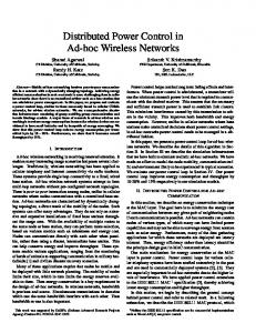
4-node topology

Three simulation scenarios are run, the first assuming a flat fading pathloss model with nominal attenuation (α = 4) having uncertainty modeled in the normally distributed noise parameter σ. For the second scenario, uncertainty is added by changing the attenuation factor from a constant to a normally distributed variable such that α ∈ Uniform(2, 6). Shadowing is added to the channel model for the third scenario as given by the following equation: Prx = Ptx d−α Ψ, Ψ ∼ LN dB(0, σ 2 ).

(6)

The robust optimal powers for all nodes in the network can be found for each simulation scenario using the optimization framework formulated in the previous section. AMPL [21], a commercial modeling framework, is used in combination with a stochastic physical layer simulator to model the wireless adhoc network. MINOS [22], a nonlinear solver, is linked to the robust formulation of the power control problem in AMPL and is used to search for the optimal power allocation vector. The tradeoff between optimality and feasibility is analyzed by two metrics as the weight ω on the penalty function increases: 1) Probability of feasibility: P (SIN Rij ≥ γ) = E [I (SIN Rij (s) ≥ γ)]

(7)

2) Power margin (cost of uncertainty): γ ω,pow =

m X i=1

Pω,pow tx

=

20 m

10 m

P∗,pow (s) tx

subject to :

Simulation Scenario. The simulation setup is a 30 meter by 20 meter arena containing a set of four manually distributed nodes. The node and link topology is shown in Figure 1. Nodes s1 and s2 are transmitters, and nodes r1 and r2 are receivers. The arrows denote the direction of desired communication channel.

i=1

subject to :

P

V. N UMERICAL AND SIMULATION RESULTS

ω,pow Ptx,i −E

m hX

∗,pow Ptx,i

i (8)

i=1

First scenario: path loss with noise uncertainty We model path loss flat fading with attenuation constant α = 4 and noise as a normal random variable. Thus: Ptx,i Aij SIN Rij = P 2 P (9) k6=i tx,k Akj + Nj j ∈ Ri , i = 1, . . . , m. N ∼ N (µ, σ 2 ) Using µ = 0.01, σ = 0.01, SIN R requirement γ = 5, and transmitting power Ptx,i ≥ 0, we run the simulation on ω ∈ [0.1, 1]. The feasibility and power margin metrics are shown in Figures 2(a) and 2(b), respectively, in relation to an increasing ω. As the feasibility measure is weighted with more importance, the probability of feasibility converges from 50% to 87% in Figure 2(a). The price for this robustness is shown in Figure 2(b), where the power margin indicates a more conservative power allocation which sacrifices optimality for a higher chance of remaining feasible. Second scenario: path loss with propagation constant uncertainty

Probability of Feasibility vs Penalty Weight

Power Margin vs Penalty Weight

0.9

0.6

0.85

0.4 0.75

Power Margin

Probability of Feasibility

0.5 0.8

0.7 0.65

0.3

0.2 0.6 0.1 0.55 0.5

0 0.1

0.2

0.3

0.4

0.5 0.6 Penalty Weight

0.7

0.8

0.9

1

0.1

(a) Scenario 1: Probability of feasibility vs. penalty weight (ω)

0.2

0.3

0.4

0.5 0.6 Penalty Weight

0.7

0.8

0.9

1

(b) Scenario 1: Power margin vs. penalty weight (ω)

Probability of Feasibility vs Penalty Weight

Power Margin vs Penalty Weight

0.55

100 90 80 70 Power Margin

Probability of Feasibility

0.5

0.45

0.4

60 50 40 30

0.35

20 10

0.3

0 0

100

200

300

400 500 600 Penalty Weight

700

800

900

1000

0

(c) Scenario 2: Probability of feasibility vs. penalty weight (ω)

100

300

400 500 600 Penalty Weight

700

800

900

1000

(d) Scenario 2: Power margin vs. penalty weight (ω)

Probability of Feasibility vs Penalty Weight

Power Margin vs Penalty Weight

1

14000 sigma = 1 sigma = 3 sigma = 5

0.9

sigma = 1 sigma = 3 sigma = 5

12000 10000

0.8 Power Margin

Probability of Feasibility

200

0.7 0.6 0.5

8000 6000 4000 2000

0.4

0

0.3

-2000 0

10000 20000 30000 40000 50000 60000 70000 80000 90000 100000 Penalty Weight

(e) Scenario 3: Probability of feasibility vs. penalty weight (ω) Fig. 2.

0

10000 20000 30000 40000 50000 60000 70000 80000 90000 100000 Penalty Weight

(f) Scenario 3: Power margin vs. penalty weight (ω)

Feasibility and power margin metrics for trade-off between optimality and feasibility of power control for Scenarios 1, 2, and 3

Keeping noise normally distributed, N ∼ N (µ, σ 2 ), uncertainty is added in the path loss exponent.

Prx = Ptx d−α , α ∈ Uniform(2, 6)

(10)

All other parameters remain unchanged from scenario 1. The range of ω is increased because the power required to achieve robustness is greatly increased and therefore a different scale for the penalty weight is required in order to observe the tradeoff between optimality and feasibility. The two metrics are shown in Figures 2(c) and 2(d). In relation to the uncertainty added by the noise, the effect of the uncertain path loss exponent was significantly greater. This result is apparent from the convergence to a lower probability of feasibility in Figure 2(c). Third scenario: path loss plus shadowing Attenuation model is extended further by incorporating shadowing as in Equation 6. Three values of the lognormal standard deviation are considered: σ ∈ {1, 3, 5}. All other parameters and sources of uncertainty are kept unchanged from scenarios 1 and 2. That is, normally-distributed noise variable and unformly-distributed path loss exponent both still contribute to the randomness in the channel model. The two metrics are shown in Figures 2(e) and 2(f). The range for the penalty weight (ω), was extended further because of added uncertainty in the attenuation model. The results show that an increase in the uncertainty of the shadowing corresponds to a greater power margin, but also to an optimal power allocation that is more robust in terms of feasibility.

Fig. 3.

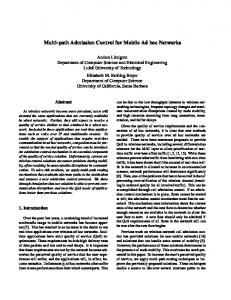
50-node network example.

VI. C ONCLUSION Our proposed robust formulation of power control in ad hoc wireless networks determines a power allocation that is maximally optimal and feasible under uncertain channel models. The small 4-node example was used to demonstrate the tradeoff between optimality and feasibility while considering channel noise, pathloss attenuation, and shadowing effects. A large-scale simulator was constructed for the modeling of the physical layer and nonlinear optimization process. Future work will be focused on analysis of scalability of robust power control with increasing simulated network size. A medium-scale example in Figure 3 shows a 50-node network generated by the simulator with Delaunay triangulation [23] used for link-topology generation.

R EFERENCES [1] A. Duel-Hallen, S. Hu, and H. Hallen, “Long-range prediction of fading signals,” IEEE Signal Processing Magazine, vol. 17, pp. 62–75, 2000.

[2] A. Arrendondo, K. Dandekar, and G. Xu, “Vector channel modeling and prediction for the improvement of downlink received power,” IEEE Trans. on Communications, vol. 50, pp. 1121–1130, July 2002. [3] I. Chlamtac, M. Conti, and J. Liu, “Mobile ad hoc networking: imperatives and challenges,” Ad Hoc Networks, vol. 1, no. 1, pp. 13–64, July 2003. [4] R. Yates, “A framework for uplink power control in cellular radio systems,” IEEE J. Selected Areas Commun., vol. 13, pp. 1341–1348, Sept. 1995. [5] G. Foschini and Z. Miljanic, “A simple distributed autonomous power control algorithm and its convergence,” IEEE Trans. Veh. Technology, vol. 42, pp. 641–646, Nov. 1993. [6] H. Su and E. Geraniotis, “Adaptive closed-loop power control with quantized feedback and loop filtering,” IEEE Trans. Wireless Commun., vol. 1, pp. 76–86, Jan. 2002. [7] J. Zander and S. L. Kim, Radio Resource Management for Wireless Networks. Boston, MA: Artech, Apr. 2001. [8] A. Yener, R. Yates, and S. Ulukus, “Interference management for cdma systems through power control, multiuser detection and beamforming,” IEEE Trans. Commun., vol. 49, pp. 1227–1239, July 2001. [9] Y. Liang, F. Chin, and K. Liu, “Power allocation for ofdm using adaptive beamforming over wireless networks,” IEEE Trans. Commun., vol. 53, pp. 505–514, Mar. 2005. [10] K. K. Leung and L. C. Wang, “Controlling qos by integrated power control and link adaptation in broadband wireless networks,” Eur. Trans. Telecommun., no. 4, pp. 383–394, July 2000. [11] Z. Han and K. Liu, “Joint link quality and power management over wiereless networks with fairness constraint and space-time dversity,” IEEE Trans. Veh. Technology, vol. 53, pp. 1138–1148, July 2004. [12] ——, “Power minimization under throughput management over wireless networks with antenna diversity,” IEEE Trans. Wireless Commun., vol. 3, pp. 2170–2181, Nov. 2004. [13] H. Su and E. Geraniotis, “Power allocation and control for multicarrier systems with soft decoding,” IEEE J. Selected Areas Commun., vol. 17, pp. 1759–1769, Oct. 1999. [14] G. Song and Y. Li, “Cross-layer optimization for ofdm wireless networks–part i:theoretical framework,” IEEE Trans. Wireless Commun., vol. 4, pp. 614–624, Mar. 2005. [15] C. Saraydar, N. Mandayam, and D. Goodman, “Efficient power control via pricing in wireless data networks,” IEEE Trans. Commun., vol. 50, pp. 291–303, Feb. 2002. [16] V. Shah, N. Mandayam, and D. Goodman, “Power control for wireless data based on utility and pricing,” in Proceedings of the Ninth IEEE International Symposium on Personal Indoor and Mobile Radio Communications, 1998, pp. 1427–1432. [17] M. Hayajneh and C. Abdallah, “Distributed joint rate and power control game-theoretic algorithms for wireless data,” IEEE Commun. Letters, vol. 8, no. 8, pp. 511–513, Aug. 2004. [18] J. Hicks, A. MacKenzie, J. Neel, and J. Reed, “A game theory perspective on interference avoidance,” in Proceedings of Globecom 2004, vol. 1, 2004, pp. 257–261. [19] J. Mulvey, R. Vanderbei, and S. Zenios, “Robust optimization of largescale systems,” Operations Research, vol. 43, pp. 264–281, March 1995. [20] Y. Wu, P. Chou, Q. Zhang, K. Jain, W. Zhu, and S.-Y. Kung, “Network planning in wireless ad hoc networks: a cross-layer approach,” IEEE Trans. J. Selected Areas Commun., vol. 23, pp. 136–151, Jan. 2005. [21] R. Fourer, D. M. Gay, and B. W. Kernighan, AMPL – A Modeling Language for Mathematical Programming. South San Francisco: The Scientific Press, 1993. [22] B. A. Murtagh and M. A. S. W. Murray, “MINOS: A solver for large-scale,” May 16 2003. [Online]. Available: http://citeseer.ist.psu.edu/587225.html; http://www.gams.com/dd/docs/solvers/minos.pdf [23] R. Sibson, “Locally equiangular triangulation,” The Computer Journal, vol. 21, pp. 243–245, 1978.