Robust Place Recognition for 3D Range Data based on Point Features. Bastian Steder .... range values in the image be rx,y, with x, y being the pixel position in ...
Robust Place Recognition for 3D Range Data based on Point Features Bastian Steder
Giorgio Grisetti
Abstract— The problem of place recognition appears in different mobile robot navigation problems including localization, SLAM, or change detection in dynamic environments. Whereas this problem has been studied intensively in the context of robot vision, relatively few approaches are available for threedimensional range data. In this paper, we present a novel and robust method for place recognition based on range images. Our algorithm matches a given 3D scan against a database using point features and scores potential transformations by comparing significant points in the scans. A further advantage of our approach is that the features allow for a computation of the relative transformations between scans which is relevant for registration processes. Our approach has been implemented and tested on different 3D data sets obtained outdoors. In several experiments we demonstrate the advantages of our approach also in comparison to existing techniques. Index Terms— Place recognition, SLAM, loop closing, point clouds, range images, range sensing
Wolfram Burgard
Score 0.85
Score 0.58
Score 0.51
Score 0.31
Fig. 1. Motivating example for the place recognition procedure. The images show 360◦ range images. The top range image was given to the system as input and the four bottom images were correctly identified as the same place. For each of these, the corresponding score for the match is given. No false positives were returned. The left two images are consecutive scans in the trajectory of the robot, the right two are loop closures, when the robot returned into that area.
I. I NTRODUCTION In the recent years, the problem of place recognition has been studied intensively in the area of mobile robotics. Techniques for place recognition are highly relevant in the context of the SLAM problem, as they can be used to solve the data association problem. They can also be applied to speed up global localization or to detect changes in the environment. Whereas the majority of place recognition techniques have been developed for vision-based navigation, there are relatively few approaches that can be applied to three-dimensional laser range scans to efficiently calculate the similarity between scans or to efficiently calculate the relative transformations between two scans. In this paper we present a novel approach to place recognition which operates on 3D laser data. Our approach transforms a given 3D range scan into a range image and calculates interest points based on a variant of the Laplacian of Gaussian method. Candidate transformations are then calculated by matching features extracted at the position of these interest points. The quality of a match between range images is then further evaluated by projecting several of the interest points into the coordinate frame of the other range image. One typical example of a range image is depicted in Figure 1. It also shows the range images and their scores as they were obtained with our algorithm from a database of range images recorded in the same area as the query scan. The entire approach described in this paper has two desirable properties. First, as the experimental results demonstrate, it is able to reliably retrieve for a given 3D scan all corresponding scans All authors are members of the University of Freiburg, Department of Computer Science, D-79110 Freiburg, Germany. {steder,grisetti,burgard}@informatik.uni-freiburg.de
taken at nearby locations. Compared to existing techniques, our method exhibits a higher recognition rate when it is trained to minimize the number of false matches. Second, our system allows for an accurate estimation of the relative transformations between the input scan and all the matches in the database and thus can provide good initial guesses for scan matching routines, which are known to be sensitive to the initialization. This paper is organized as follows. After discussing related work we will describe our approach in Section III. In Section IV we then will present experimental results based on two different datasets obtained in outdoor environments. II. R ELATED W ORK In the past, the problem of place recognition has been addresses by several researchers and a wide variety of approaches for different types of sensors have been developed. One very successful and recently developed approach in this area is the Feature Appearance Based MAPping algorithm (FABMAP) proposed by Cummins and Newman [5]. This algorithm uses a bag-of-words approach based on SURF features [3] extracted from omni-directional camera images. Cummins and Newman evaluated their method on two extremely large-scale datasets including a 70km and a 1000km trajectory recorded with a car. For the 70 km dataset they achieved a 48.4% recall rate. For the 1000 km dataset they report a rate of 3.1% (respectively with no false positives), which is still enough for a graph-based SLAM algorithm to create a proper map. The query time for a new image is about half a second. However, most of the required computation time is spent for the feature extraction. We would like to
refer the reader to this paper for a detailed discussion of vision-based place recognition approaches. In the area of place recognition with 2D range scans, Granstr¨om et al. [6] proposed a machine learning approach to detect loops. A combination of rotation-invariant features is extracted from the scans and a binary classifier based on boosting is used to recognize previously visited locations. Bosse and Zlot [4] also presented a loop closing solution for 2D range data. They build local maps from consecutive 2D scans for which they compute histogram-based features. The correlation between these features is than used to match the local maps against each other. An approach that is similar to ours regarding the utilization of point features to create candidate transformations is described in the PhD thesis of Huber [10]. His approach extracts Spin Images [11] from 3D scans and uses them to match each scan against a database. In our previous work [15] we demonstrated, that the features we use in this paper are more descriptive than Spin Images in the context of object recognition. Huber reported 1.5 s as the time requirement to match one scan against another. Even considering the advances in computer hardware since 2002, our approach is substantially faster (about factor 80). Recently, Magnusson et al. [14] proposed a system for place recognition based on 3D data. They utilize the Normal Distribution Transform as features to match scans. These features are global appearance descriptors, which describe the whole 3D scan instead of just small areas as it is the case for our features. They report impressive results regarding the matching time per scan pair (below 0.1 ms). However, their recall rates are substantially lower than ours. Additionally, in contrast to their approach, our method is able not only to identify similar places, but also to directly return the location of the robot within the corresponding scans. In the experimental results section we will compare our approach to theirs based on a freely available dataset (see Section IV-B). III. P LACE R ECOGNITION USING R ANGE I MAGES The goal of our approach is to retrieve those 3D scans from a database that are most similar to a given query scan. We represent all scans as range images. A range image is an image, in which each pixel contains the depth returned by a laser beam passing through that pixel. In the remainder of this section we will use the terms “scan” and “range image” interchangeable. To retrieve scans similar to a given query scan, our system compares the current measurement with all scans in the database using an efficient feature based search algorithm. We then calculate candidate transformations between the query scan and the scans in the database. We assign a score to each candidate transformation by comparing significant points in the scans and the similarity of two scans is the maximum of the scores for all found candidate transformations. In the following we will explain the individual steps in more detail.
A. Feature Extraction Our feature extraction algorithm operates in two phases: We first identify the so-called interest points of the query scan. Afterward, we extract a descriptor vector for each of these points. These descriptors are later used to compare two features. We calculate the descriptor vector of the features according to the procedure described in our previous work [15]. In particular, we extract a local interpolated range image patch from a view point lying along the normal of an interest point. This constrains 5 of the 6 degrees of freedom of the relative transformation between the two range images. We resolve the remaining degree of freedom (the rotation around this normal) by orienting the patch along the zaxis in the world, i.e., the simulated viewers orientation is along the normal and upright in the world. This method effectively removes the invariance to the roll of the robot pose. This restriction did not have any noticeable effect in the datasets used in our experiments, since the robot was moving on mostly flat ground. The feature descriptor covers a fixed 3D distance around the point it was extracted from. In our experiments we used a radius of 1.25 m and the size of the range image patches was 10 × 10 pixels. Since the features encode a complete 3D transformation, knowing a single feature correspondence between two scans, we are able to retrieve all 6 degrees of freedom of the relative transformation between them. As interest points, we would like to select those pixels of the range image which represent areas that are substantially different from their surrounding. In our previous work, we used a standard Harris detector [8] calculated directly on the range images to find interest points. Whereas this appears to be an effective solution, the Harris detector in its original form is designed for vision and not for range images. If it is applied without any modification to a range image, its reaction to points is not invariant to the distance of the pixel. Additionally, interest points that lie on the border of an object might be placed on the pixels in the background instead of the ones in the front. In this work we therefore propose a novel method that is based on the Laplacian of Gaussian (LoG) method [12] and analyzes the second derivative of the depth values in the range image. Let the range values in the image be rx,y , with x, y being the pixel position in the image. The gradient in x at pixel x, y can be ∂ rx,y ≈ rx+1,y − rx−1,y and the approximated as Gxx,y = ∂x ∂ y gradient in y as Gx,y = ∂y rx,y ≈ rx,y+1 − rx,y−1 . To gain invariance regarding the depth at which the interest point lies, we normalize the gradient as follows: � � Gxx,y ′ 2 x · (1) Gx,y = arctan tan(α) · r(x, y) π � � Gyx,y ′ 2 y · (2) Gx,y = arctan tan(α) · r(x, y) π where α is the angular resolution of the range image. This term is connected to the impact angle γ of the � sensor beam � Gx,y π on the obstacle surface by γ ≈ 2 − arctan tan(α)·r(x,y) .
The factor π2 scales the value to [-1,1]. G′x,y = 0.0 means that the neighboring ranges are equal and a value of 1.0 marks a jump to infinity. We calculate the second derivative of the gradient of Eq. 2 in the image as Gx2 x,y Gy2 x,y
′
′
′
′
x x = Gx+1,y − Gx−1,y
=
y Gx,y+1
−
x Gx,y−1
The interest value I(x, y) ∈ [0, 1] is then defined as: q y2 2 2 I(x, y) = (Gx2 x,y ) + (Gx,y ) .
(3) (4) Fig. 2. Example of the interest point extraction procedure on the scan of a Teddy bear. The points are at positions where the gradient changes significantly and does not lie on a straight line.
(5)
I(x, y) = 0 corresponds to a planar surface and higher values mark possible interest points characterized by a high curvature. To reduce the effect of sensor noise, we apply a Gaussian convolution to G′x,y , before calculating G2x,y . The above procedure also gives high interest values to certain points, that should not be used for feature extraction, like the shadows of occlusions or straight edges which do not represent corners in the sensed surface. To reject these points as interest points we apply the following filtering procedure: i) Occlusions: When one object occludes another, the points at the border of the occluded area in the background object will receive a high interest value, since there is a high change of a substantial gradient. However these features are typically not stable since they are viewpoint dependent. We identify such points because of their high normalized gradient (close to 1.0) and since they have a greater range value than their neighbors. For these points we set the interest value to 0.0. ii) Points on a line: Our procedure returns all points where there is an abrupt change in gradient and will capture all the points lying on the edge of an object. However, if these points lie on a straight line, they are not salient for the matching. Therefore, we calculate the angle of the dominant direction of the change in the gradient at each image point using Gx2 and Gy2 , effectively finding the local direction of the line on which the points lie. We keep only pixels as interest points, where the neighboring pixels in the determined direction have different angles. This change marks corners, since all pixels on a straight line will have very similar angles. After applying these two filters, the interest points are determined as all local maxima whose interest value lies above a certain threshold. Figure 2 shows an example of the interest point extraction process. Additionally, to keep the number of extracted features small, we restrict the minimal distance between interest points in 3D, since close obstacles can have many interest points on them. In our experiments we found that a minimum distance of 0.5 m provides appropriate point sets. B. Calculation of Candidate Transformations For each 3D scan, we calculate the range image and extract the features as described in the previous section. The resulting features are then stored in a database. For a typical 3D scan obtained with our robot, that contains up to 200,000
data points, the features obtained with our algorithm require about 200 KB per scan. To match a query scan against the database, we compare all the features in the scan with the features in the database using the Euclidean distance between their descriptors. We consider all pairs of features whose descriptors distance is below a certain threshold as possible feature matches. To perform this procedure in an efficient way, we store all feature description vectors in a kd-tree and apply the best-bins-first strategy proposed by Lowe [13] to handle the high dimensionality of the vectors. We then use the resulting feature correspondences between two scans to calculate candidate transformations between the scans, which are the 6DOF displacements between the robot poses. Since the features encode a complete transformation between the scan coordinate system and the feature coordinate system, one correspondence is enough to determine the transformation between the scans. Yet, using multiple correspondences increases the accuracy of the result. Using at least three feature correspondences one can compute the 3D transformation between the scans using standard least square minimization methods (see, e.g., Horn et al. [9]). For two correspondences, one can use an additional virtual point per feature, lying on an arbitrary position in the feature coordinate system, thereby reducing it to a four point correspondence problem. Unfortunately, the number of possible combinations grows exponentially with the number of correspondences. Additionally, in some cases, where the overlap between scans is small, there might only be a very small number of correct feature matches available. Therefore, to restrict the number of created candidate transformations but still maximize the chances of finding the correct ones, we calculate a fixed number of transformations for different numbers of feature correspondences. During our experiments, we used 500 transformations for one, two, and three feature correspondences respectively, resulting in a maximum of 1,500 candidate transformations between two scans. We can efficiently reject outliers in the matching by exploiting some constraints (e.g., distance) between the features in the same image and checking that this constraint is not violated by the matches as described in our previous work [15]. C. Scoring of Candidate Transformations To evaluate how well two scans match given a candidate transformation, we analyze the re-projection of a fixed num-
ber n (100 in our implementation) of points into the other coordinate frame. We call these points validation points. It is important that these points have some significance in the scene and are not just selected randomly, or two scans could get a high score, just because the floor or a big wall is matched well. To avoid this problem, we employ the interest points (see Section III-A), that were already calculated during the feature extraction phase. We select a subset of the interest points V = {v1 , · · · , vn }, containing points that are as equidistant as possible. We then transform these points into the coordinate system of the other scan, which results in the set of points V ′ = {v1′ , · · · , vn′ }. Now we project each point vi′ into the range image of the second scan, leading to the range value ri and the pixel position (xi , yi ). Next we want to compare the range of our validation point with the actual range value at that position in the image rxi ,yi . To avoid that slight errors in the estimation of a correct transformation lead to a very small score, e.g., if the point lies on an obstacle border and we hit the much further away neighbor instead, we consider not only (xi , yi ), but also its neighbors in a small error radius e ∈ N (2 in our implementation) around it. This leads to the set N = {(x, y)
|
x ∈ {xi − e, · · · , xi + e}, y ∈ {yi − e, · · · , xy + e}}.
(6)
Since we are mostly interested in image points with ranges that are similar to ri we also define the subset ˆ N ′ = {(x, y) | (x, y) ∈ N ∧ |rx,y − ri | ≤ d},
(7)
where dˆ is the maximum allowed error for the difference in range (we used 0.3 m). The next step is to calculate a score for each validation point. This score should have the following properties: If there are no points in the image at this position (the area was not visible), the score should be 0.0. If the area is visible, but non of the range values there are similar, we would like to give this a penalty of −p (which corresponds to -0.3 in our implementation). If there are similar range values, we would like to obtain a score between zero and one, according to how similar the value is and how far x′ , y ′ is away from xi , yi Taking these requirements into account, we define the following scoring function for a single validation point: 0.0, if N = ∅ ′ −p, if � ∅ � N = ∅ ∧ N 6= s(vi ) = |rx′ ,y′ −ri | max · λx′ ,y′ , else 1− dˆ ′ ′ ′ (x ,y )∈N
(8) where λx′ ,y′ ∈ (0.0, 1.0] is a weighting factor that is based on how far x′ , y ′ is away from xi , yi . In our implementation we use 0.25 λx′ ,y′ = 0.75 + p , (9) ′ 2 (x − xi ) + (y ′ − yi )2 + 1 which is actually a value between 0.75 and 1.0. When the score for all validation points is calculated, we can sum them up to get the score S ∈ [0, 1] for the candidate
transformation: 1 S = · max 0.0, n
n X
!
s(vi )
i=0
(10)
The resulting score is then used to decide if the candidate transformation is valid. To achieve this, we introduce a threshold, which was set to 0.25 in all our experiments. This value was found as a bound above which we did not encounter any false positives in our datasets. IV. E XPERIMENTS In this section, we present the real-world experiments carried out to evaluate our approach. For the first experiment we used a self-recorded dataset that we acquired on our campus using a wheeled robot equipped with a SICK LMS laser range scanner mounted on a pan-tilt unit. The pan-tilt unit was moved to acquire a 360◦ view of the surrounding. The scans were obtained in a stop-and-go fashion and it takes our platform about 25 s to capture a scan. The dataset contains 77 3D scans captured along a 723 m long trajectory. The average distance between the captured scans was about 10 m and we used a maximum range of 50 m for the laser measurements. Figure 3 shows an overlay of the trajectory over an aerial image. Each scan consists of 150,000-200,000 points. The resolution of the range images we extracted from the scans was 0.5◦ per pixel. We made this dataset freely available (see [1]). Additionally, we used the freely available Hanover2 dataset (Courtesy of Oliver Wulf) which has also been used by Magnusson et al. [14] to evaluate their place recognition system. It contains 923 3D scans acquired along a 1.24 km long path. Fig. 5 depicts an overlay of the trajectory over a corresponding aerial image. Each scan covers 360◦ and contains about 15,000 points. We extracted range images from these scans with a resolution of 1.3◦ per pixel. The average distance between the captured scans was about 1.5 m and the maximum range for the measurements was 30 m. More information about the dataset can be found on the corresponding web site [2]. To obtain trajectories close to the ground truth, we used the graph mapping approach TORO [7]. The edges were created from the odometry of the robot and from 3D scan matching, whereas every scan match was verified by a human. A. Freiburg Campus Figure 3 gives an overview over the area and the trajectory obtained by the standard SLAM algorithm. From each scan, 50-200 features were extracted. For this dataset we calculated the confusion matrix illustrated in Figure 4(a). Each scan was matched against all others and the corresponding cell in the matrix visualizes the score of the best transformation between the two scans. We used a score of 0.25 as the acceptance threshold to decide whether a transformation is considered correct in all our experiments. The dark areas that are not close to the main diagonal, mark loop closures. Here the system was able to
Fig. 3. Trajectory of the Freiburg dataset overlayed on a Google Earth image of our campus. This trajectory was acquired using odometry and hand checked scan matching as edges in a graph SLAM system. The crosses mark the positions of the robot where the scans for the localization experiment were captured.
match scans from different times, where the robot visited the same area (Compare with Figure 3). Figure 4(b) gives an overview over the number of true positives and false negatives and the resulting recall rate as a function of the distance between scans. On this dataset the recall rate of our system is above 90% for locations closer than 15 m. A high recall rate for large distances between scans is important, since it allows to retrieve the robot’s pose, even if its position is not exactly on the former trajectory. Figure 4(c) plots the number of false positives and the recall rate for a maximum distance of 15 m between scans as a function of the acceptance threshold. Beyond a score of 0.188 no false positives remain. Thus, our default acceptance threshold of 0.25 is well in the area containing no false positives. To test the ability of our system to localize the robot using a newly acquired scan, we placed our robot on 20 different locations on our campus and acquired a scan. From these scans, 10 were obtained in areas for which there was no corresponding scan in the database. The other 10 scans were close to the trajectory taken by the robot while the database was created (see Fig. 3). Our system correctly identified all 10 places that were close to places in the database and also rejected the other 10 scans as unknown. To evaluate the quality of the transformations between the scans we compared the output of our system for the best matching place in the database with the manually verified result of an ICP based scan matcher. The average translational error was 0.16 ± 0.05m and the average orientation error was 0.75 ± 0.27◦ . B. Hanover2 Dataset Figure 5 gives an overview over the area and the trajectory obtained by the standard SLAM algorithm for this dataset. As for the other dataset, the trajectory was created using a graph mapping approach based on the odometry given in the dataset and manually performed 3D scan matching. Our algorithm extracted 50-100 features from each scan . The lower number of features results from the much lower resolution of the scans. However, relative to the size of the range images, the
Fig. 5. Trajectory of the Hanover2 dataset overlayed on a Google Earth image. This trajectory was acquired using odometry and hand checked scan matching as edges in a graph SLAM system.
number of features is higher, since there are more complex structures in this dataset like trees, which typically increases the number of interest points. For this dataset we also calculated the confusion matrix, which is illustrated in Figure 6(a). Again we used a score of 0.25 as the minimum threshold to decide if a transformation is considered correct. Figure 6(b) gives an overview over the number of true positives, false negatives and the resulting recall rate depending on the distance between the scans. For this dataset, the recall rate of our system is above 85% for locations closer than 5 m. Figure 6(c) shows the development of the false positives and the recall rate for a maximum distance of 5 m between scans depending on the score threshold. There are no false positives starting from a score above 0.235, so our threshold of 0.25 again guarantees no false positives. Magnusson et al. [14] used a distance of 10 m as the visibility constraint for the evaluation of their recall rate of 35.3%. For this distance our recall rate is 58.1%. C. Timings The time requirements for a database query are mainly linearly dependent on the number of scans in the database. Additionally, there is an overhead for each query that depends on the size of the input scan and the number of features extracted from the scan. For the two datasets we performed our experiments on we obtained the following timings on a 2.4 GHz Dual-core Pentium PC, using only a single core. For the Freiburg dataset the calculations necessary for every scan (creation of the range image and feature extraction) took 1.02 s on average. The calculation of the complete confusion matrix took 151 s, which means that we need about 1.96 s to match a scan against the database. Thereby, the feature matching took about 180 ms. Therefore, the pairwise comparison of two scans (disregarding feature extraction and matching) took 23 ms. Note that for our robot, the time requirements to match a scan against the database is minor compared to the time it takes to capture a scan. For the Hanover dataset the calculations necessary for every scan (creation of the range image and feature extraction) took 0.48 s on average. The calculation of the complete
0.6
30
0.4
40
0.2
50
0
350
true positives false negatives recall rate
300
80
60
250
60
200 150
40
100 20
70
50
0
100
0 10 20 30 40 50 60 70 80
(a)
20
80
15
60
10
40
5
20
0
0
0
0 5 10 15 20 25 30 35 40 Maximum distance to neighbor scans in m
80
25
false positives recall rate
No. of false positives
20
100
Recall rate in %
0.8
No. of true positives/false negatives
1
10
Recall rate in %
0
0
0.2
0.4
0.6
0.8
1
Minimal score to consider two scans as matches
(b)
(c)
Fig. 4. (a): The confusion matrix of the Freiburg dataset. 77 3D scans were acquired and the matrix shows the scores of the pairwise comparisons that were above 0.25. (b): The number of true positives, the number of false negatives, and the resulting recall rate for different maximum distances between scans to consider them overlapping for the Freiburg dataset. (c): Number of false positives and the recall rate for different minimum scores for the Freiburg dataset. There are no false positives starting from a score above 0.188. The recall rate is determined regarding a maximum distance of 15 m between scans. 100
0.8
200 0.6
400
0.4
500
0.2
600
0
700
80 Recall rate in %
300
true positives false negatives recall rate
1000 0 100 200 300 400 500 600 700 800 900 1000
(a)
70000 60000 50000
60
40000 40
30000 20000
20 10000
800 900
80000
0
0
0 5 10 15 20 25 30 35 40 Maximum distance to neighbor scans in m
(b)
100
5000
false positives recall rate
4000
80
3000
60 40
2000
20
1000
No. of false positives
1
Recall rate in %
100
No. of true positives/false negatives
0
0
0 0
0.2
0.4
0.6
0.8
1
Minimal score to consider two scans as matches
(c)
Fig. 6. (a): The confusion matrix of the Hanover2 dataset. A total number of 923 3D scans were acquired and the matrix shows the scores of the pairwise comparisons with a score larger or equal to 0.25. (b): The number of true positives, the number of false negatives, and the resulting recall rate for different maximum distances between scans to consider them overlapping for the Hanover2 dataset. (c): Number of false positives and the recall rate for different minimum scores for the Hanover2 dataset. There are no false positives starting from a score above 0.235. The recall rate is determined regarding a maximum distance of 5 m between scans.
confusion matrix took 4 h 39 min, which means that we needed about 18.14 s to match a scan against the database, of which the feature matching took about 1.1 s. Therefore, the pairwise comparison of two scans (disregarding feature extraction and matching) took 18 ms. V. C ONCLUSIONS In this paper we presented a robust approach for 3D place recognition using range images, that also produces highly accurate relative pose transformations between two scans. Our system employs a novel interest point extractor specifically designed for range images. The obtained interest points are applied to extract features and to score candidate transformations. We evaluated our approach on real world data acquired on our campus and also on one freely available dataset. While our computational requirements are higher than those of other state-of-the-art systems, our recall rate on the considered datasets is substantially higher. In future work, we plan to substantially reduce the computational cost of our method by introducing fast pre-selection methods for the scan candidates, e.g., using a bag-of-words approach like Cummins and Newman [5] or by using the approach of Magnusson et al. [14] with a high difference threshold as a preprocessing method. ACKNOWLEDGMENTS We thank Oliver Wulf, Leibniz University, Hanover, Germany for providing the Hanover2 dataset and Rainer K¨ummerle for providing us with his scan matching software.
R EFERENCES [1] Dataset of 360◦ 3D scans of the Faculty of Engineering, University of Freiburg, Germany. http://ais.informatik.uni-freiburg.de/projects/datasets/fr360. [2] Hanover2 dataset. http://kos.informatik.uni-osnabrueck.de/3Dscans. [3] H. Bay, T. Tuytelaars, and L. Van Gool. SURF: Speeded up robust features. In Proc. of the Europ. Conf. on Comp. Vision (ECCV), 2006. [4] M. Bosse and R. Zlot. Map matching and data association for largescale two-dimensional laser scan-based slam. International Journal of Robotics Research, 27(6):667–691, 2008. [5] M. Cummins and P. Newman. Highly scalable appearance-only SLAM FAB-MAP 2.0. In Proc. of Robotics Science and Systems (RSS), 2009. [6] K. Granstr¨om, J. Callmer, F. Ramos, and J. Nieto. Learning to detect loop closure from range data. In Proc. of the IEEE Int. Conf. on Robotics & Automation (ICRA), 2009. [7] G. Grisetti, C. Stachniss, and W. Burgard. Non-linear constraint network optimization for efficient map learning. 2009. In press. [8] C. Harris and M. Stephens. A combined corner and edge detector. In Proceedings of The Fourth Alvey Vision Conference, 1988. [9] B. K. P. Horn. Closed-form solution of absolute orientation using unit quaternions. Journal of the Optical Society of America. A, 4(4):629– 642, Apr 1987. [10] D. Huber. Automatic Three-dimensional Modeling from Reality. PhD thesis, Robotics Institute, Carnegie Mellon University, Pittsburgh, PA, December 2002. [11] A.E. Johnson and M. Hebert. Using spin images for efficient object recognition in cluttered 3d scenes. IEEE Trans. Pattern Anal. Mach. Intell., 21(5):433–449, 1999. [12] T. Lindeberg. Feature detection with automatic scale selection. International Journal of Computer Vision, 30(2):77–116, 1998. [13] D.G. Lowe. Object recognition from local scale-invariant features. In Proc. of the Int. Conf. on Computer Vision (ICCV), 1999. [14] M. Magnusson, H. Andreasson, A. N¨uchter, and A.J. Lilienthal. Appearance-based loop detection from 3D laser data using the normal distributions transform. In Proc. of the IEEE International Conference on Robotics and Automation (ICRA), pages 23–28, 2009. [15] B. Steder, G. Grisetti, M. Van Loock, and W. Burgard. Robust online model-based object detection from range images. In Proc. of the Int. Conf. on Intelligent Robots and Systems (IROS), 2009.