Chris Schwarz was born in Moline, IL, in 1968. He received the B.S. degree in electrical engineering from the University of Illinois, Urbana-Champaign, in 1990 ...
2088
IEEE TRANSACTIONS ON SIGNAL PROCESSING, VOL. 46, NO. 8, AUGUST 1998
Robust Relative Stability of Time-Invariant and Time-Varying Lattice Filters Soura Dasgupta, Fellow, IEEE, Minyue Fu, and Chris Schwarz
Abstract— We consider the relative stability of time-invariant and time-varying unnormalized lattice filters. First, we consider a set of lattice filters whose reflection parameters �i obey j�i j � �i and provide necessary and sufficient conditions on the �i that guarantee that each time-invariant lattice in the set has poles inside a circle of prescribed radius 1=� < 1, i.e., is relatively stable with degree of stability ln �: We also show that the relative stability of the whole family is equivalent to the relative stability of a single filter obtained by fixing each �i to �i and can be checked with only the real poles of this filter. Counterexamples are given to show that a number of properties that hold for stability of LTI Lattices do not apply to relative stability verification. Second, we give a diagonal Lyapunov matrix that is useful in checking the above pole condition. Finally, we consider the time-varying problem where the reflection coefficients vary in a region where the frozen transfer functions have poles with magnitude less than 1=� and provide bounds on their rate of variations that ensure that the zero input state solution of the time-varying lattice decays exponentially at a rate faster than 1=�1 > 1=�:
and
(1.3) In the sequel, the LTI version of (1.1)–(1.3) will refer to the equals a constant for all case in which each In this case, will be the transfer function Since we are interested in relative stability, we first make precise our notion of relative stability. As we deal with systems that are time varying, we use a state variable realization (SVR)based approach to stability analysis. Definition 1.1 (Relative Stability): Consider the LTV sys, i.e., obeying tem with SVR
Index Terms— Lattice filters, Lyapunov, robustness, stability, time-vaying filters.
I. INTRODUCTION
(1.4) (1.5) and are, respectively, and bounded matrices, the state is , and and are the input and output signals, respectively. Then, (1.4)–(1.5) is relatively stable with a degree of stability if there exist constants such that the zero input state solution obeys for all and initial time
where
T
HIS PAPER explores the relative stability of linear timeinvariant (LTI) and linear time-varying (LTV) lattice filters. Lattice filters have been studied extensively in the last two decades. They bear a direct relationship to the celebrated Levinson–Durbin algorithm [1] and have been applied in speech processing and linear predictive coding [2]. An th-order Lattice filter is depicted in Fig. 1, where is the unit delay element. are called the reflection coefficients; the Here, the time index used with these recognizes our intention to study is a unit delay. As is evident the time-varying lattice, and from this figure, the various signals obey, for (1.1) for (1.2) Manuscript received April 5, 1996; revised January 21, 1998. This work was supported in part by NSF Grants ECS-9350346 and ECS-9211593. The associate editor coordinating the review of this paper and approving it for publication was Dr. Victor E. DeBrunner. S. Dasgupta and C. Schwarz are with the Department of Electrical and Computer Engineering, University of Iowa, Iowa City, IA 52242 USA. M. Fu is with the Department of Electrical and Computer Engineering, The University of Newcastle, Callaghan, Australia. Publisher Item Identifier S 1053-587X(98)05217-9.
(1.6) where If
denotes the standard 2-norm. , (1.6) implies (1.7)
ensures Thus, relative stability with degree of stability that the zero input state response decays at an exponential rate If (1.6) holds, we will sometimes say that of at least , then we simply call (1.4)–(1.5) is stable. If, in (1.6), (1.4)–(1.5) stable. and are constant), In the LTI case (where (1.4)–(1.5) has transfer function (1.8) is completely reachable and In this case, as long as completely observable (see [13] for definitions), then has poles with magnitude less (1.4)–(1.5) is stable iff , i.e., is stable. than
1053–587X/98$10.00 1998 IEEE
DASGUPTA et al.: ROBUST RELATIVE STABILITY OF TIME-INVARIANT AND TIME-VARYING LATTICE FILTERS
Fig. 1.
It is known that in the LTI case, where the lattice filter is stable iff
2089
Lattice filter.
for all (1.9)
Furthermore, under (1.2), the lattice transfer function (1.10) is allpass, i.e., it obeys for all (1.11) There are, however, two outstanding open issues in the understanding of lattice filters. The first of these concerns the issue of relative stability of the LTI lattice. Simply put, what are the conditions on the reflection coefficients that ensure the stablity of the LTI lattice? Such relative stability, as opposed to mere stability, is important in most practical applications as it reduces the likelihood of quantization induced limit cycles. Further, as will become evident in the sequel, the relative stability of the LTI lattice is also critical to the stability of the LTV lattice. The second concerns the relative stability of the LTV lattice. It is known that the normalized version of the above lattice [3], [4] is stable under arbitrary time variations in the reflection coefficients as long as they obey (1.12) However, to our knowledge, no nontrivial conditions exist that guarantee the stability, let alone the relative stability, of the LTV unnormalized lattice structure of Fig. 1. In fact, it is well known that the unnormalized LTV lattice could be unstable, despite the satisfaction of (1.12) [4]. This paper considers relative stablity of both the LTI and the LTV lattices depicted in Fig. 1. The two problems addressed are as follows. Problem 1.1: In Fig. 1, the ’s are all time invariant, and for some
Find sufficient conditions on the rate of variations in the such that for some , this LTV lattice is stable. In analyzing LTV systems, it is, in general, unreasonable to assume complete knowledge of the nature of the time variations. Normally, the knowledge we have is limited to the extent and rate of parameter variations. Equation (1.14) characterizes the extent of variation. Problem 2 then calls for specification of the variation rate. Observe that effectively, the statement of Problem 2 ensures the stability of all possible frozen LTI lattices corresponding to the LTV lattice being analyzed. Problem 1 addresses the condition under which all such frozen LTI lattices will be stable. Subject to this condition on the frozen LTI lattices, Problem 2 then calls for determining the parameter variation rates that ensure relative stability with a smaller degree Although it is important in its own right, Problem 1 is therefore also useful to the analysis of LTV lattices. In Problem 2, there and the allowable is clearly a natural tradeoff between stability is preserved. For rate of time variation for which a given , the larger the , the greater the permissible rate. Our solution to Problem 2 captures this tradeoff, very much in the spirit of [5]. Translated to the digital filter framework, [5] considers digital filters in the direct form. It gives bounds on the logarithmic rate of variation of the filter coefficients that guarantee the relative stability of the underlying LTV system, subject to a relative stability assumption on the frozen systems. In particular, [5] assumes that the denominator coefficients of the frozen LTI system transfer functions are and that the time-varying values of these obey, for some (1.15) and that all LTI frozen systems defined by (1.16) Recall that the are stable for some in the direct-form implementations. Then, with
directly appear
(1.17)
(1.13) so that Find necessary and sufficient conditions on the are stable with for all , as in (1.13). , every LTI system Problem 1.2: Suppose for some obeying (1.13) is stable. Now, suppose the reflection coefficients in Fig. 1 vary with time and obey for some arbitrarily small (1.14)
stable with the LTV filter is shown in [5] to be if there exist and such that (1.18) Here else.
(1.19)
2090
IEEE TRANSACTIONS ON SIGNAL PROCESSING, VOL. 46, NO. 8, AUGUST 1998
Note the tradeoff between the degree of the frozen system , the LTV filter degree of stability , relative stability and the average rate of variation in the parameters directly monotonically related to the filter coefficients ; the Further, only increases in and, increase with the are of concern. Diminishing carry no hence, destabilizing influence. A result of this nature is sought here for the LTV lattice of Fig. 1. In Section II, we provide some preliminaries. Section III gives a series of results connected to Problem 1. Section IV develops a Lyapunov matrix needed in the solution to Problem 2. Section V then solves Problem 2. Section VI is the conclusion.
Proposition 2.1: Consider the set of polynomials
(2.5) continuous functions of and for all Then, all members of are Schur (have zeros strictly inside the unit circle) iff one member is Schur and for all
with
(2.6) II. PRELIMINARIES This section derives a number of preliminary results and definitions. First, we define the technical concept of uniform complete observability (UCO) [9], which is needed for some of our analysis. and Definition 2.1: The pair of matrix sequences , respectively, and , is called UCO if there and integer such that for all exist
We next present a recursive formula for determining the transfer function of a lattice filter. In the sequel (see Fig. 1), we will define (2.7) and for (2.8) Thus
(2.1) Here, the products are identity should the lower index exceed the upper, and the order is exemplified by
(2.9) which is the overall transfer function of the lattice. Then, we have, from [12], that for all
(2.10) We next recount a fact from stability theory that provides the principle tool to be used in out LTV analysis. Theorem 2.1 [6]: Consider (1.4)–(1.5) with the various quantities defined in Definition 1.1. Then, (1.6) holds iff there Lyapunov matrix satisfying exists a symmetric
Further, we will define the transfer function sets (2.11) (2.12)
(2.2) for which (2.3) real and UCO. In the LTI case of with will be constant as well. constant Much of our analysis relies on the concept of bounded real (BR) transfer functions defined below. Definition 2.2: An LTI system with transfer function is BR if is stable and for all (2.4) An important tool in robust stability analysis of LTI systems is the zero exclusion principle [11], which is presented below.
Finally, we present a similar result for LTV lattice SVR’s. In the sequel, unless necessary, we will drop the explicit dependence on the Define to be an SVR of the and output , as in Fig. 1 system with input [i.e., the system that in the LTI case has transfer function ]. The state vector is the output of the delay elements appearing in the system and is given by (2.13) In
Theorem
2.1,
we
provide
recursions that relate to for The recursion is initiated with in (2.7), the nondynamic system corresponding to and are zero dimensional objects, i.e., and
DASGUPTA et al.: ROBUST RELATIVE STABILITY OF TIME-INVARIANT AND TIME-VARYING LATTICE FILTERS
Theorem 2.2: Consider, with , the SVR of the system with input and output in Fig. 1, with state vector , as in (2.13). Then (2.14) (2.15) (2.16) (2.17) where the
vector
obeys (2.18)
Proof: By definition (2.19) (2.20)
2091
III. ROBUST RELATIVE STABILITY OF THE LTI LATTICE We call a set of transfer functions stable invariant if all its members are stable. In this section, we provide a necessary to be stable invariant, and sufficient condition for Thus, this solves the problem of determining given has degree of stability whether each member of In addition, where appropriate, we will point out certain salient points on which -stability properties differ from mere stability. A third contribution of this section is to answer the following question. Are there any distinguished members of whose stability implies the stability of all members ? of It is known that for any is stable iff for all is stable. Example 3.1 shows this not to be the case for stability in general. Example 3.1: Consider the lattice filter as in Fig. 1 and (1.1) with
Further, from (1.1) (2.21) From Fig. 1, (2.20), and (2.21)
(2.22) Thus, substituting into (2.19), we have
Then, we can verify that Yet, all
is stable for is unstable for all
Nonetheless, Lemma 3.1 below shows that when it comes , an to verifying the stable invariance of the entire set order reductibility property does hold. is stable invariant iff Lemma 3.1: The set is stable invariant for all Proof: Sufficiency is clear. To prove necessity, assume is not stable that for some such invariant. Then, there exists is unstable. Now, observe that Thus (3.1)
(2.23) Observe from (2.10) that
Since, by the definition (2.13), this proves (2.14), (2.15). Further, from (1.1)
(3.2)
(2.24) This proves (2.16)–(2.17) because of (2.18). An important consequence of this theorem is that if , then (2.25) Together with the initiating process stated just before the theorem statement, this provides the SVR of the lattice filter in Fig. 1. As an illustration, observe that
(2.26)
is unstable. Hence, we have Thus, the result. The fact that the order reductability property applies to even for is stable invariance of sets such as contain crucially dependent on the fact that the sets elements involving Henceforth, we consider the stable invariance of all the We are now in a position to state the main result of this section. This result requires that (3.3) (3.4) be considered. Then, the necessary and sufficient condition for is as follows. the stable invariance of the
2092
IEEE TRANSACTIONS ON SIGNAL PROCESSING, VOL. 46, NO. 8, AUGUST 1998
Theorem 3.1: Consider the sets , as is stable defined in (2.8)–(2.12). Then, with defined in (3.3)–(3.4) exist and obey, for invariant iff the all
Lemma 3.2: Suppose the set and Then, for all
is stable invariant. exist (3.12)
and (3.5) Further, under (3.5), for all (3.6)
The proof of this result is developed in the sequel. However, before embarking on this proof, we make a few pertinent observations. , the recursion in (3.3)–(3.4) gives Note that with for all , and (3.5) boils down to
(3.13) Proof: Use induction. First, observe that (3.12) guarNow, clearly antees the existence of and all exists. Suppose for some exists. Then, as (3.12) holds at and for , its violation will imply that for some (3.14) For this choice of (3.15)
(3.7) which is a fact well known about lattice filters. Note, however, that (3.7) is necessary and sufficient for stability of any , whereas (3.5) is not necessary for the Indeed, return to the filter stability of is stable for in Example 3.1. Yet, for this value of , taking
and
3.1 illustrates a further departure from case. Despite the fact that for the given is stable for all is unstable for Thus, although the stability of a solitary lattice filter is determined entirely by the magnitude of the reflection coefficients, this is not the case for the relative stability of a solitary lattice filter. Observe that (3.6) implies that
as otherwise, choice of
, which violates , from (3.11)
Thus, for this (3.16)
Observe from (2.7), (2.10), (3.10), and (3.11) (3.17) has a pole at 1, and is Hence is not not stable invariant. Then, from Lemma 3.1, stable invariant. The contradiction proves (3.12). To prove (3.13), again use induction. Suppose it holds for Then, because of (3.10), some
Example the
(3.8) whence we have that a necessary, although not sufficient, is condition for stable invariance of (3.9) Finally, observe that the number of computations needed to check the condition in question grows only linearly with We now turn to proving this theorem through a series of lemmas. The first of these concerns a sequence related to the
(3.10) (3.11)
(3.18) Clearly, the satisfaction of (3.12)–(3.13) is a necessary From (3.11), condition for the stable invariance of it is also sufficient for the existence of the for all Comparing (3.10)–(3.11) with (3.3)–(3.4), we find that for all (3.19) exist. Thus, we have shown should, of course, the following. is stable invariant only if the Lemma 3.3: The set in (3.3)–(3.4) exist and obey (3.5). Further, (3.6) also holds. Remark 3.1: An interesting consequence of Lemma 3.3 is the fact that the violation of (3.5) is equivalent to the has a member with pole requirement that for some In view of this, must also have a member with at a pole at Henceforth, we will assume that (3.5), and thus (3.6), holds.
DASGUPTA et al.: ROBUST RELATIVE STABILITY OF TIME-INVARIANT AND TIME-VARYING LATTICE FILTERS
Lemma 3.4: Consider (3.3)–(3.4) and (3.10)–(3.11). Suppose the exist and that (3.5) holds. Then, for all and , the exist
2093
Now, observe under (3.26)
(3.28)
(3.20) and (3.12)–(3.13) holds. Proof: Clearly, should (3.20) hold and the exist, then must exist, and as , (3.12) must hold. We use the Now, induction to prove (3.20). This clearly holds at Then suppose it holds at some
because of (3.26) and the facts that lower bound in (3.23) holds at with respect to maximum of
(3.29)
(3.21) whence from (3.11), Further,
exists.
Thus, the Consider next the
, and , the maximum Thus, because of (3.26), occurs according to the following rule: At
, from whence
if if
(3.30)
In either case, because of (3.26) Further, observe that as
and (3.31)
Thus, as (3.22) The fact that (3.13) holds follows similarly to the proof of Lemma 3.2. The next lemma points to a BR result. Lemma 3.5: Consider (3.3), (3.4), (3.10), and (3.11), with Suppose (3.5) holds for all Then, for all , and for all (3.23) Proof: That the first two inequalities imply (3.23) is a consequence of Lemma 3.4. Observe also from this Lemma exist and obey that (3.24) Now, use induction. From (2.7), (3.23) clearly holds for Now, suppose it holds at for some Then, at any , there exist dropping the arguments and such that
Then, (3.23) follows from (3.11). We can now prove the sufficiency part of the theorem. as defined Lemma 3.6: Consider the sets in (2.8)–(2.12) and the sequence as in (3.3)–(3.4). Suppose exist and for all obey (3.5). Then, for all the is stable invariant. is stable Proof: We use induction. Clearly, is stable invariant for some invariant. Now, suppose Observe that all elements of have Further, from (3.2) degree
is stable for all Thus, from Proposition is not stable invariant only if there exists 2.1, such that for some (3.32) i.e., because of (2.10) (3.33)
(3.25) with
i.e., because of Lemma 3.5 (3.26) (3.34)
Now, at this
from (2.10), with
(3.27)
violating (3.12). Thus, Lemmas 3.3 and 3.6 prove Theorem 3.1. We conclude this section with two results of independent interest. The proof of the first follows from Lemma 3.5 and the fact that BR systems are stable.
2094
IEEE TRANSACTIONS ON SIGNAL PROCESSING, VOL. 46, NO. 8, AUGUST 1998
Theorem 3.2: The set and
is stable invariant iff for all
because
and
(3.35) and (3.36) are BR. Further, for all (3.37) Compare this with the allpass property when The next theorem relates the stable invariance of to the stability, in fact, the real poles, of a “worst” member. The Theorem 3.3: Given following are equivalent. is stable invariant. 1) The set is stable. 2) has no poles on 3) The proof of the Theorem relies on the following Lemma. has no poles in Lemma 3.7: Suppose Then
Proof: Since pass. Thus, with
Since that
is stable all-
It follows from induction that are all negative. Consequently, If , Case II: , and follows from induction. then or Note that In either case, By Lemma 3.7, this cannot happen. must hold. Hence, Therefore, all exist and obey (3.5). Thus, Theorem 3.3 shows that the stability invariance of boils down to the stability of a single the whole set , the set of corner Lattice filter. Recall that when stability preserving lattice coefficients form Therefore, it is intuitive to conjecture a convex set that the result in Theorem 3.3 can be generalized to the case where the set of reflection coefficients lie in a nonsymmetric interval, i.e.,
has real coefficients, it readily follows
Suppose Since has no poles on , the only way changes sign as travels from to 1 is if there exists some such that
Using (2.10), we have
or (3.38) , which We proceed to show that (3.38) implies To see this by induction, we assume, for contradicts , that some
Indeed, (2.10) gives
Proof of Theorem 3.3: Since 1) implies 2) and 2) implies 3), it suffices to show that 3) implies 1). In view of Theorem 3.1, it suffices to show that 3) implies that exist and obey (3.5). We proceed by contradiction. Obviously, exists. Suppose 3) holds. Assume that exists, , for all and some and but that Case I: Then
We show via the following example that when the parameter set becomes nonsymmetric, relative stability of corner filters will not imply the relative stability of the whole set. Example 3.2: It is straightforward to is stable at but unstable at verify that Note from this example that even lies in a does not. symmetric interval, although Remark 3.2: Condition 3) in Theorem 3.3 offers a simple for which relative way of determining the maximum is guaranteed for all stability of Indeed, is the smallest pole of on the positive real axis, which can be checked easily by solving the in Theorem 2.2. real eigenvalues of IV. LYAPUNOV MATRIX FOR RELATIVELY STABLE LTI LATTICES In order to address the LTV problem considered in Section V, we need to determine a Lyapunov matrix that It is known [7] that proves the stable invariance of with
(4.1)
DASGUPTA et al.: ROBUST RELATIVE STABILITY OF TIME-INVARIANT AND TIME-VARYING LATTICE FILTERS
and
, the SVR of (4.2)
, we need to However, for the stable invariance of that obeys find a positive definite symmetric
2095
of (3.10)–(3.11), the Lyapunov matrix in (4.4) depends only on as opposed to depending on directly. The rest of this section is devoted to proving Theorem 4.1. and as defined in Theorem 2.2 (we are With assuming time invariance here), the transfer function
(4.3) , where is a completely for observable pair. The main result of this section, which is presented below, solves this problem. is stable invariant Theorem 4.1: Suppose Then, with , the SVR of with , and defined by
(4.10) In
other
words,
has SVR Accordingly, we will call the
realization matrix of (4.11)
(4.4) , we have
for all
and
Observe from Theorem 2.2 that
(4.5) are as in (3.10)–(3.11). We have dropped the Here, the in and arguments Observe from (3.10), Lemma 3.2, and (2.12) that the stable ensures that is positive definite for invariance of Further, from Lemma 3.2 all
(4.12) Our proof of Theorem 4.1 will use induction. To this end, note from Theorem 3.2 that the stable invariance of implies that for all and all is BR. Consequently, matrix from [14], it follows that there exists a
(4.6) Thus,
in (4.3) is
(4.13) such that with
(4.7)
(4.14)
Further, observe that
(4.15) (4.8)
where
.. .
(4.9)
is Then, it is readily verified (see the Appendix) that positive definite throughout Observe that as for all , whenever , we recover the result of [7] when A few further comments on the nature of the derived Lyapunov matrix are in order. In the setting of [5] involving directform realization, the Lyapunov matrix was multiaffine in the coefficients of the transfer function denominator. This fact considerably simplified the LTV analysis conducted in [5]. The Lyapunov matrix in (4.4) is clearly not multiaffine. There is, however, one vast simplification in the form of (4.4) over its counterpart in [5], namely, that it is diagonal. As will be shown in Section V, this diagonal nature aids the LTV analysis conducted there. Two other points to be exploited in Section V is independent of Further, because are as follows. First,
Then, the next Lemma shows that Observe that acts as a Lyapunov matrix for the stability verification of Lemma 4.1: Suppose that is stable and for some is as in (4.13)–(4.15), with (4.11) in force. Then (4.16) Proof: Because of (4.15) and (4.13)
(4.17) Hence, we have the result. Clearly, the stable invariance of and Lemma 3.2 ensures that the left-hand side of (4.16) is negative semidefinite. The next step of the induction argument must relate to To this, we need two intermediate Lemmas. The first of these relates the positive semidefiniteness of a special class matrices. of matrices to the definiteness of certain
2096
IEEE TRANSACTIONS ON SIGNAL PROCESSING, VOL. 46, NO. 8, AUGUST 1998
Lemma 4.2: Consider scalars Then
and
as in (2.18).
Lemma 4.4: Suppose is stable invariant with Consider as in Lemma 4.1. Define
(4.18)
(4.28)
iff
and (4.19) (4.29)
Proof: Consider Then, (4.16) is equivalent to
to be scalar. Then (4.20)
for all
This in turn is equivalent to (4.21)
Hence, we have the result. The next Lemma gives some key properties of Lemma 4.3: Suppose that is stable invariant with Then, under (3.10)–(3.11), for all
(4.30) case separately from the Proof: We will treat the case. In this case, from (3.11) Case I: (4.31) Further, from Theorem 2.2 and (4.11)
(4.22)
(4.32)
and (4.23)
From (4.28) and (4.31) (4.33)
Proof: From (3.10), (3.11), and Lemma 3.2 Thus
(4.34)
(4.24)
matrix
Define the
Further
Note that
Because of (4.11)
(4.25) (4.35)
Then, (4.22) follows easily. Now, from (3.11)
(4.26)
Moreover, because of (4.14) (4.36)
Thus Thus, from (4.34)–(4.36)
(4.27) hence, we have the result. We are now in a position to proceed with the inductive step to of relating
the last inequality following from (4.15). Hence, the result holds.
DASGUPTA et al.: ROBUST RELATIVE STABILITY OF TIME-INVARIANT AND TIME-VARYING LATTICE FILTERS
Case II: 2.2
Because of (2.25), (4.11), and Theorem
2097
Finally, from Lemmas 4.3 and 3.2 (4.45)
(4.37)
Then, it is readily verified using Lemma 4.3 that (4.46)
Observe through direct verification that Consequently, (4.4) together with (4.45) implies that (4.42) holds. Hence, (4.30) holds. Then, the proof of Theorem 4.1 follows by noting that (4.38) Observe from (4.14) that (4.39) Because of (4.37) and (4.39), (4.30) is, in turn, equivalent to
and hence, Then, with the induction so initiated, we can repeatedly use Lemmas 4.1 and 4.4 to obtain the desired result that (4.47) V. RELATIVE STABILITY
OF THE
LTV LATTICE
This section addresses the relative stability of LTV lattice arbitrarily small filters. We will assume that there exists such that for all and (4.40), shown at the bottom of the page. Because of (4.16) and (4.39), (4.30) is guaranteed, provided we have (4.41), shown at the bottom of the page. Observe from Lemma 4.2 that this is equivalent to (4.42), shown at the bottom of the as in (4.28). Then, using (4.2), the (1, page. Now, select 1) block of (4.42) equals
(5.1) We will further assume that the in (3.3)–(3.4) obey (3.5) for , i.e., all frozen systems are stable with degree all The question is, given of stability (5.2)
(4.43) where the last equality is from Lemma 4.2. Likewise (4.44)
what rates of time variations can be sustained to ensure that ? the LTV Lattice has degree of stability To this end, we present two results. The first is a simple consequence of the comments made at the end of the previous section. The second constitutes the main result of this section.
(4.40)
(4.41)
(4.42)
2098
IEEE TRANSACTIONS ON SIGNAL PROCESSING, VOL. 46, NO. 8, AUGUST 1998
Theorem 5.1: Consider the lattice filter depicted in Fig. 1. is stable invariant Suppose that (5.1) holds and that Suppose also that there exist such that for for some and all all (5.3)
Proof: Consider the Lyapunov matrix and observe that (5.5) prevails. Note that two and obey matrices
in (5.4), diagonal (5.11)
Then, the LTV lattice filter is stable with degree of stability
, the th diagonal of is less than or iff for all Then, from (5.4), it is readily equal to the th diagonal of is the smallest scalar for which observed that
Proof: Suppose is the SVR of the lattice filter as exemplified in Theorem 2.2. Define
(5.12)
(5.4)
The “ ” notation in (5.10) accounts for the fact that the elements of both and equal 1. the state vector of the lattice (see Theorem 2.2), With consider the zero input state solution of
Observe that because of Lemma 3.2, (3.10), (3.11), and (5.1), such that for all there exists (5.5)
(5.13) Consider (5.14)
Further, because of (5.3) and (3.10)–(3.11) (5.6)
Then, because of (5.5), it suffices to show that under (5.10), such that along (5.13), for all there exists
Then, because of Theorem 4.1 (5.15) (5.7)
is a bounded Now, observe that under our assumptions, matrix. Hence, (5.13) cannot have finite escape time. In fact, such that for all because of (5.5) along (5.13), there exists
(5.8)
(5.16)
Then, we show in the Appendix that
Hence, obeys (2.1). Note that (5.8) is real for all we have the result. Observe that this theorem states that as long as the frozen , the LTV filter LTI systems have degree of stability sustains the same degree of stability for arbitrary rates of as long as the sustain variation in only changes in sign, and (5.1) holds for all The next theorem addresses relative stability under simultaneous magnitude variations in multiple reflection coefficients. Theorem 5.2: Consider the LTV lattice in Fig. 1, which is stable invariant and that obeys (5.1). Suppose that Then, the LTV lattice is stable with degree of stability obeying (5.2), if the following holds: There exists an integer and such that
Now, consider
(5.17) Then, because of Theorem 4.1 (5.18) Then, the recursive application of (5.18) reveals that for all
(5.9) where
(5.19) where the last inequality is because of (5.9). Then, because of (5.16), for all
(5.20)
(5.10) Hence, we have the result.
DASGUPTA et al.: ROBUST RELATIVE STABILITY OF TIME-INVARIANT AND TIME-VARYING LATTICE FILTERS
A few comments concerning (5.9)–(5.10) are now appropriate. Essentially, this condition represents a tradeoff between frozen systems and LTV system degree of stability with the Sign changes rate of variations in the magnitude of the are inconsequential. Observe that with
2099
and (A.5) the matrix in (2.1) is has the form (2.16) that
Observe from (2.14) and
(5.21) (A.6) (5.22) Thus, (5.9)–(5.10) essentially quantify the potentially destabiand limit lizing time variations as those that increase Declining values of the average increase in these are found not to be destabilizing. VI. CONCLUSION We have studied the relative stability of both the LTI and the LTV lattice. We have shown that when the LTI set of lattice filters is defined by bounds on the reflection coefficients, then there is a simple necessary and sufficient condition for all such We also show that LTI lattices to have degree of stability verification of stable invariance can be effected by checking a single corner of We provide a Lyapunov matrix for checking this degree of stability requirement and show that it specializes to the matrix of [7]. Finally, we give a logarithmic rate of variation result that suffices for the relative stability of LTV unnormalized lattices. Although the LTI results of Section III apply to the normalized lattice as well, the LTV and Lyapunov results do not. An important issue is a generalization that captures this normalized case. APPENDIX This appendix shows that is UCO for and defined in Theorem 2.2 and (5.8), respectively. When are LTI, the UCO property of implies that in (4.8) is positive definite. In (2.1), choose Call (A.1) Observe from Lemma 3.4 that because of the stable invariance of
is real for all and, , obeys for some (A.2)
Then, with diag
(A.3)
.. .
(A.4)
is where th element
upper triangular with the
Thus, is triangular with the property that its Further, for all element is zero whenever th element is its
th ,
(A.7)
Clearly, since elements in (A.7) are bounded away from zero and, hence, are bounded, and all elements of (2.1) holds. REFERENCES [1] B. D. O. Anderson and J. B. Moore, Optimal Filtering. Englewood Cliffs, NJ: Prentice-Hall, 1979. [2] J. R. Deller, J. G. Proakis, and J. H. L. Hansen, Discrete-Time Processing of Speech Signals. New York: Macmillan, 1993. [3] A. H. Gray and J. D. Markel,“A normalized digital filter structure,” IEEE Trans. Acoust. Speech, Signal Processing, vol. ASSP-23, pp. 268–277, June 1975. [4] S. Phoong and P. P. Vaidyanathan, “Time-varying filter banks: Factorizability of lossless time-varying filters and filter banks,” Tech. Rep., Calif. Inst. Technol., Pasadena, Apr. 1995. [5] S. Dasgupta, G. Chockalingam, B. D. O. Anderson, and M. Fu, “Lyapunov functions for uncertain systems with applications to the stability of time varying systems,” IEEE Trans. Circuits Syst., vol. 41, pp. 93–106, Feb. 1994. [6] J. C. Willems, Stability Theory of Dynamical Systems. London, U.K.: Nelson, 1970. [7] M. Mansour, “A note on the stability of linear discrete systems and Lyapunov method,” IEEE Trans. Automat. Contr., vol. AC-27, pp. 707–708, June 1982. [8] B. D. O. Anderson, E. I. Jury, and M. Mansour, “Schwarz matrix properties for continuous and discrete time systems,” Int. J. Contr., vol. 23, pp. 1–16, 1976. [9] V. L. Kharitonov, “Asymptotic stability of an equilibrium position of a family of systems of linear differential equations,” Differ. Equ., vol. 14, pp. 1483–1485, 1979. [10] B. D. O. Anderson and J. B. Moore, “Detectability and stabilizability of time-varying discrete-time linear systems,” SIAM J. Contr. Optimiz., vol. 19, pp. 20–32, Jan. 1981. [11] S. Dasgupta, P. J. Parker, B. D. O. Anderson, F. J. Kraus, and M. Mansour, “Frequency domain criteria for the robust stability of linear and nonlinear dynamical systems,” IEEE Trans. Circuits Syst., vol. 38, pp. 389–397, 1991. [12] S. K. Mitra, P. S. Kamat, and D. C. Huey, “Cascaded lattice realization of digital filters,” Circuit Theory Applicat., vol. 5, pp. 3–11, 1977. [13] K. J. Astr¨om and B. Wittenmark, Computer-Controlled Systems. Englewood Cliffs, NJ: Prentice-Hall, 1990. [14] K. Zhou, J. C. Doyle, and K. Glover, Robust and Optimal Control. Englewood Cliffs, NJ: Prentice Hall, 1996.
2100
Soura Dasgupta (M’87–SM’93–F’98) was born in 1959 in Calcutta, India. He received the B.E. degree in electrical engineering from the University of Queensland, Brisbane, Australia, in 1980 and the Ph.D. degree in systems engineering from the Australian National University, Canberra, in 1985. He is currently Dean’s Diamond Professor of Electrical and Computer Engineering at the University of Iowa, Iowa City. In 1981, he was a Junior Research Fellow in the Electronics and Communications Sciences Unit at the Indian Statistical Institute, Calcutta. He has held visiting appointments at the University of Notre Dame, Notre Dame, IN, University of Iowa, Universit´e Catholique de LouvainLa-Neuve, Louvain, Belgium, and the Australian National University. His research interests are in controls, signal processing, and neural networks. Dr. Dasgupta served as an Associate Editor of the IEEE TRANSACTIONS AUTOMATIC CONTROL between 1988 and 1991. He was a corecipient of the Gullimen Cauer Award for the best paper published in the IEEE TRANSACTIONS ON CIRCUITS AND SYSTEMS in 1990 and 1991, is a Presidential Faculty Fellow, and is an Associate Editor for the IEEE Control Systems Society Conference Editorial Board.
Minyue Fu received the Bachelors degree in electrical engineering from the China University of Science and Technology, Hefei, in 1982 and the M.S. and Ph.D. degrees in electrical engineering from the University of Wisconsin, Madison, in 1983 and 1987, respectively. From 1983 to 1987, he held a Teaching Assistantship and a Research Assistantship at the University of Wisconsin, Madison. He worked as a Computer Engineering Consultant at Nicolet Instruments, Inc., Madison, WI, during 1987. From 1987 to 1989, he served as an Assistant Professor in the Department of Electrical and Computer Engineering, Wayne State University, Detroit, MI. During the summer of 1989, he was employed by the Universit´e Catholoque de Louvain, Louvain, Belgium, as a Maitre de Conferences Invited. He joined the Department of Electrical and Computer Engineering, the University of Newcastle, Callaghan, Australia, in 1989, where he now holds an Associate Professorship. His main research interests include robust control, dynamical systems, stability, and signal processing. Dr. Fu has been an Associate Editor of the IEEE TRANSACTIONS ON AUTOMATIC CONTROL and an Associate Editor for the Conference Editorial Board of the IEEE Control Systems Society.
IEEE TRANSACTIONS ON SIGNAL PROCESSING, VOL. 46, NO. 8, AUGUST 1998
Chris Schwarz was born in Moline, IL, in 1968. He received the B.S. degree in electrical engineering from the University of Illinois, Urbana-Champaign, in 1990 and the Ph.D. degree in electrical engineering from the University of Iowa, Iowa City, in 1998. From 1991 to 1993, he worked for J. J. Majon Consultants, Grayslake, IL. He is presently employed by National Advanced Driving Simulator, Iowa City. His research interests include control systems and digital signal processing, especially involving linear time-varying systems.