Robust Sliding Mode Control for Robot Manipulators - IEEE Xplore

2444

IEEE TRANSACTIONS ON INDUSTRIAL ELECTRONICS, VOL. 58, NO. 6, JUNE 2011

Robust Sliding Mode Control for Robot Manipulators Shafiqul Islam, Member, IEEE, and Xiaoping P. Liu, Senior Member, IEEE

Abstract—In the face of large-scale parametric uncertainties, the single-model (SM)-based sliding mode control (SMC) approach demands high gains for the observer, controller, and adaptation to achieve satisfactory tracking performance. The main practical problem of having high-gain-based design is that it amplifies the input and output disturbance as well as excites hidden unmodeled dynamics, causing poor tracking performance. In this paper, a multiple model/control-based SMC technique is proposed to reduce the level of parametric uncertainty to reduce observer– controller gains. To this end, we split uniformly the compact set of unknown parameters into a finite number of smaller compact subsets. Then, we design a candidate SMC corresponding to each of these smaller subsets. The derivative of the Lyapunov function candidate is used as a resetting criterion to identify a candidate model that approximates closely the plant at each instant of time. The key idea is to allow the parameter estimate of conventional adaptive sliding mode control design to be reset into a model that best estimates the plant among a finite set of candidate models. The proposed method is evaluated on a 2-DOF robot manipulator to demonstrate the effectiveness of the theoretical development. Index Terms—Adaptive control, output feedback, robotics, robust control.

I. I NTRODUCTION

O

VER THE PAST few decades, the sliding mode control (SMC) technique for a class of nonlinear mechanical systems has been studied extensively by many researchers (see [1], [5], [8], [10], [13], [14]–[23], [26], [31], [37], [41], [45], to name a few). The main idea of employing the SMC approach is to cope with the parametric uncertainties for the complex multiinput multi-output (MIMO) nonlinear systems. If we assume that the unknown parameters and initial conditions become large values, then the existing single-model (SM)-based SMC designs either for state or output feedback exhibit poor tracking performance. To improve the tracking response, one may use high observer-controller gains to increase the convergence of the state and parameter estimates. More specifically, the statefeedback-based classical SMC approach requires high learning gains as well as high discontinuous control gains to obtain fast convergence of the parameter estimator. In the output feedback case, high observer-controller gains are essential for the robust reconstruction of the state and parameter estimates to achieve good tracking performance. However, the demand

Manuscript received October 5, 2008; revised March 31, 2009 and August 28, 2009; accepted April 12, 2010. Date of publication July 29, 2010; date of current version May 13, 2011. This work was supported in part by the Natural Science and Engineering Research Council of Canada, Canada Research Chairs Program and Research Excellence in Science and Engineering Award from Carleton University. The authors are with the Department of Systems and Computer Engineering, Carleton University, Ottawa, ON K1S 5B6, Canada (e-mail: sislam@sce. carleton.ca). Digital Object Identifier 10.1109/TIE.2010.2062472

of high observer-controller gains makes the SM-based output feedback SMC design even more complex in real-time applications since high observer speed amplifies the input and output disturbance, causing high-frequency chattering and the infinitely fast switching control phenomenon. As a consequence, the existing design for the state or output feedback may not be practically implementable as control efforts in most practical systems are limited. On the other hand, high observer-controller gain may excite unmodeled high-frequency dynamics as well as amplify the disturbance uncertainty associated with the input and output, resulting in poor tracking performance. To deal with the problem associated with high observercontroller gains, we introduce a multiple model/control technique for robust tracking control problem for MIMO robotic systems. Results in this area for a class of single-input singleoutput (SISO) nonlinear systems can be found in [2], [11], [27], [29], and [30]. In [11], the Lyapunov-based switching technique using the multiple parameters model (MPM) is considered for the certainty equivalent (CE) [7] principle-based adaptive state feedback control problem for uncertain discrete-time SISO systems. Their idea is to use the Lyapunov-function and its incremental differences, which are independent of unknown parameters for each candidate controller. The performanceindex-based switching scheme is employed to pick the candidate controller that best approximates the plant. Authors in [27], [29], and [30] introduced multiple model technique to deal with the problem associated with the control chattering phenomenon in the SMC design. Their methods are similar to the one proposed in [11]. However, these methods assumed that the position-velocity signals are available for multiple candidate controller design. In this paper, we propose velocityindependent multiple model/control technique for robust trajectory tracking control for MIMO nonlinear mechanical systems. We first introduce a pre-routed switching-logic technique, where an inequality for the derivative of the Lyapunov function is used as a resetting criterion. It shows that the pre-ordered switching nature may cause undesirable transient tracking in the presence of a large number of candidate controllers. To improve the transient tracking performance from pre-routed switching-logic, we allow the parameter estimates to be reset instantaneously so that the control system can improve the overall tracking performance at any instant. This idea can be described as follows. First, we subdivide the compact set of uncertain parameters into smaller compact subsets, and then construct a candidate controller corresponding to each of these smaller parameter subsets. Then, at each instant, we compare a family of candidate controllers to see which candidate generates a guaranteed decrease in the value of the Lyapunov inequality. If the controller that is currently acting in the loop satisfies the Lyapunov inequality (resetting inequality), then we apply

0278-0046/$26.00 © 2010 IEEE

ISLAM AND LIU: ROBUST SLIDING MODE CONTROL FOR ROBOT MANIPULATORS

it to the system. Otherwise, the logic switches to the candidate control that best approximates the plant. The proposed design is applicable for both the full state and partial state measurement cases. The rest of the paper is organized as follows. In Section II, we formulate the problem associated with the SMbased SMC approach, which is the motivation of this paper. In Section III, the multiple parameter model-based SMC design is proposed to achieve the desired output tracking response with relatively smaller controller-observer gains as well as to reduce the control chattering phenomenon from the classical SMC approach. This section also presents nonlinear simulation results to demonstrate the efficiency of the proposed algorithm. Finally, Section IV concludes the paper.

II. P ROBLEM F ORMULATION In this section, we illustrate the problem associated with the SM-based SMC approach. To begin, let us first consider the equation of motion for n-link rigid robot [34], [36], [44] given by M (q)¨ q + C(q, q) ˙ q˙ + G(q) = τ

(1)

where q ∈ n is the joint position vector, q˙ ∈ n is the joint velocity vector, q¨ ∈ n is the joint acceleration vector, τ ∈ n is the input torque, M (q) ∈ n×n is the symmetric and uniformly positive definite inertia matrix, C(q, q) ˙ q˙ ∈ n is the coriolis and centrifugal loading vector, and G(q) ∈ n is the gravitational loading vector. The system model (1) can be defined in the error-state space form as follows: e˙ 1 = e2 , e˙ 2 = φ1 (e, qd , q˙d ) + φ2 (e1 , qd )τ − q¨d

(2)

where e1 = (q−qd ), e2 = (q− ˙ q˙d ), e = [eT1 , eT2 ]T , φ1 (e, qd , q˙d ) = −1 ˙ q˙ + G(q)], and φ2 (e1 , qd ) = M −1 (q). We −M (q)[C(q, q) consider that the desired trajectory qd (t) and its first and second derivatives are bounded as Qd = [qd , q˙d , q¨d ]T ∈ Ωd ⊂ 3n with compact set Ωd . We also consider the following well-known properties of the robot dynamics [6], [35], [38], [43], and many others: 1) M (q) ∈ Rn×n is a symmetric, bounded, and positive definite matrix with respect to joint position that satisfies the following inequalities, M (q) ≤ MM and M −1 (q) ≤ MM I , where MM and MM I are known bounded constants; 2) the matrix M˙ (q) − 2C(q, q) ˙ is skew-symmetric; and 3) the norm of the gravity and centripetal-coriolis forces are upper bounded and can be represented as C(q, q) ˙ ≤ ˙ and C(q, q˙d ) ≤ kcd q˙d ≤ kc , where CM , kcd , and CM q kc are known bounded positive constants. Let us define the reference state vector as q˙r = (q˙d − λe1 ), where λ = diag[λ1 , λ2 , . . . , λn ] with λi > 0 ∀ i = 1, 2, 3, . . . , n. Then, we can define the sliding surface as S = (e2 + λe1 ). The control objective is to drive the joint position q(t) to the desired position qd (t). This objective can be achieved by selecting an input τ such that the sliding surface satisfies the sufficient condition as (1/2)(d/dt)Si2 ≤ −ηi |Si |, where ηi is a positive constant [13], [19]. This condition implies that the energy of S will be decaying as long as S = 0. To meet the desired control

2445

objective, we consider the control law for the robot system (1) as [13] ˆ =M ˆ (q)¨ ˆ q) ˆ qr + C(q, ˙ q˙r + G(q) − KS − Ksgn(S) τ (e, Qd , θ) ˆ , and Cˆ are the estimates of M (q) where q¨r = q¨d −λe2 , M and C(q, q) ˙ and K = diag[K1 , K2 , . . . , Kn , ], K = diag[K1 , K2 , . . . , Kn ] with Ki > 0 ∀ i = 1, 2, 3, . . . , n and Ki > 0 ∀ i = 1, 2, 3, . . . , n. Now, using the control law, we can simplify the closed-loop dynamics as M S˙ +(C +K)S = β − ˆ ˆ −M )¨ = Ksgn(S), where β = (M qr +(Cˆ −C)q˙r +(G−G) ˆ M q¨r + C q˙r + G with M = M − M , C = Cˆ − C ˆ − G. We now use the Lyapunov-like function and G = G candidate V = (1/2)S T M S to establish the tracking error convergence condition for the perviously mentioned closedloop model. As M is symmetric and positive definite, then V > 0 for S = 0. Then, function V can be considered as an indicator of the energy for S. Let us now show that the energy V decays as long as S = 0. To do that, we take the derivative along the closed-loop trajectory and then use property 2 to obtain V˙ as V˙ = −S T KS − ni=1 (Si [Ki sgn(|Si |) − βi ]). n Now, if i=1 (Si [Ki sgn(|Si |) − | βi |]) ≥ 0, then we can ˙ write V as V˙ − S T KS ≤ 0. Then, the Lyapunov function can be viewed as an energy indicator for S. This implies the decay of the energy of S as long as S = 0. Thus, the sufficient condition given by (1/2)(d/dt)Si2 ≤ −ηi |Si | is satisfied. To reduce the control-chattering activity, we approximate the high-frequency switching function sgn(.) by using a smooth bounded saturation function sat(.) [3], [4], [19]. The analysis presented previously is based on the strict assumption that all the state variables are available for feedback. The implementation difficulty of the position-velocity-based SMC design is that they require velocity signals in addition to joint position signals. The main practical problem is that advanced system removes the velocity sensors to reduce the weight and cost. To obtain the velocity signals, the common practical approach is to differentiate the position measurements obtained from encoders or resolvers, which are often contaminated by severe noise [3], [4]. The quantization effect of the noisy signal may produce undesirable oscillations in the joint, which may render the unstable control system. To deal with this practical problem, some output feedback-based designs have been reported in the literature [6], [7], [9], [12], [15]– [18], [25], [38]–[40], [43], and many others, where the velocity signal is estimated by the output of the estimator. These designs can be grouped into linear and nonlinear observer-based output feedback design. In this paper, we consider linear observer to reproduce unknown velocity signals. Then, the output feedback ˆ =M ˆ (q)¨qˆr + C(q, ˆ eˆ2 + SMC can be written as τ (ˆ e, Qd , θ) ˆ ˆ − K(ˆ e2 + λˆ e1 ) − Ksat(S/φ), where eˆ is q˙d )qˆ˙ r + G(q) H1 H2 e˜1 , eˆ˙ 2 = 2 e˜1 eˆ˙ 1 = eˆ2 +

(3)

qˆ˙ r = q˙d − λˆ e1 , ¨qˆr = q¨d − λˆ e2 , Sˆ = eˆ2 + λˆ e1 , e˜1 = e1 − eˆ1 , e˜2 = e2 − eˆ2 , is a small observer design constant to be specified, H1 and H2 are positive definite matrices. The observer (3) is an independent of the system dynamics, control inputs, and uncertain model parameters. The level of uncertainty in the

2446


SM-based SMC design can be reduced by adding an adaptation term to develop an adaptive sliding mode control (ASMC) as ˆ = Y (e, q˙r , q¨r )θˆ − KS − Ksat S τ (e, Qd , θ) φ ˙ θˆ = −ΓY T (e, q˙r , q¨r )S

(4)

where θˆ is an estimate of uncertain parameters representing the inertial parameters of robot arms and its load, Y (e, q˙r , q¨r )θˆ = ˆ (q)¨ ˆ q) ˆ M qr + C(q, ˙ q˙r + G(q), Γ = diag[Γ1 , Γ2 , . . . , Γn ] with constant diagonal elements Γi > 0 ∀ i = 1, 2, 3, . . . , n and Y (e, q˙r , q¨r ) is the regressor matrix. The parameter estimates θˆ can be adjusted with the smooth parameter projection scheme ˙ ˆ Ψ)] for θ ∈ Ω = {θ|a ≤ θ ≤ b}} with [46] as θˆ = [P roj(θ, Ψ = −ΓY T (e, q˙r , q¨r )S, and δ > 0 is chosen such that θ(t) ∈ Ωδ , where Ω ⊂ Ωδ with Ωδ = {θ|a − δ ≤ θ ≤ b + δ}. The above ASMC design is implementable only when all the process states are measurable. To relax this strict assumption, we can replace the unknown state vectors in the ASMC by the output of the estimator (3) to formulate the adaptive output feedback sliding mode control (AOFBSMC) as Sˆ ˆ ˙ ¨ ˆ ˆ e, qˆr , qˆr )θ − KS − Ksat τ (ˆ e, Qd , θ) = Y (ˆ φ ˙ ˆ e, qˆ˙ r , ¨qˆr )S. θˆ = −ΓY T (ˆ

(5)

Using perturbation analysis, we can show that the performance achieved under adaptive state feedback-based SMC can be recovered asymptotically by the adaptive output feedback SMC design. This means that for the given set of initial conditions of interest, the controller under state feedback-based design (4) can be recovered by using output feedback design (5). This performance recovery has two steps [12]. In the first step, we design the SMC as a state feedback control law such that it meets the desired tracking objectives. In the second step, we replace the unknown velocity state vector in the SMC design by the output of the observer (3), and show that the domain of attraction under the state feedback SMC design can be recovered by using an output feedback sliding mode design. The performance recovery analysis can be shown by using the singular perturbation method, which has also two parts. In the first part, it is proven that there exists a short transient period T1 () ∈ [0, T2 ] during which the fast variable η approaches a function of the order O(), while the slow variables (e, θ) remain in a subset of the domain of attraction. Using the Lyapunov-like function candidate V = (1/2)S T M S, we can show that there always exists a finite time T2 independent of such that for all t ∈ [0, T2 ], V (t) ≤ c where 0.5λ2 M 0.5λM T Ωc = {e|e Qsm e ≤ c} with Qsm = . 0.5I 0.5M In the second part, the boundedness of the signal e(t) can be shown for all t ∈ [T1 (), T3 ], where T3 ≥ T2 is the first time (e(t), θ(t)) exists from the subset Ωb of Ωc with c > b. This implies that the state variables (e(t), θ(t)) remain bounded for all t ≥ T3 . This proof makes use of the fact that the fast variable η is of the order O(). To show that, we can choose a Lyapunov

function W (η) = η T P η [12] for the fast observer error model dynamics η˙ = B[−¨ qd + φ1 (e, qd , q˙d ) + φ2 (e1, qd )τ (e − −H1 I ˆ ζ()η, Qd , θ)]+A , ζ() = o η, where Ao = 0 −H 2 n×n 0 In×n 0n×n , B = n×n , η1 = e˜1 , and η2 = e2 − 0 In×n In×n eˆ2 = e˜2 . Then, it is not hard to show that the fast variables converge to the set Ω = {η|W (η) ≤ 2 β}, where β = qd +φ1 (e, qd , q˙d )+ 16P 2 k12 λmax . (P ) = 16P 3 k12 with [−¨ ˆ ≤ k1 for some k1 > 0, φ2 (e1 , qd )τ s ((e−ζ()η), Qd , θ)] P = λmax . (P ), and P is the solution of the Lyapunov equation as P Ao + ATo P = −I for all t ∈ [T1 (), T3 ]. Then, we can show that the state trajectory (e, θ) is trapped inside the set, which can be made very small by using a small value of observer design constant as V˙ ≤ −λmin . (Π)e2 + χ

(6)

with χ > 0. This implies that for the given set of initial conditions of interest, there exists an observer-controller gain such that all the signals in the closed-loop system are bounded. Notice from (6) that the design parameter represents the bandwidth of the observer dynamics and plays a vital role in achieving semiglobal property. For the given set of initial conditions of interest, we can find the minimum bound on by using a Lyapunov-like function candidate as Vc = ((1 − d)/2)S T M S + (d/2)η T P η with d > 0. Then, differentiate Vc with respect to the time along the perturbed closed-loop trajectory to simplify V˙ c as α2 V˙ c ≤ −(1 − d)α1 e2 + (1 − d)ζ1 eη − d η2 + 2dηP γsp η + 2dηP γs e s ˆ ˆ ≤ where ζ1 = ςo k1 ksm1 , ςo = λ, τ s (ˆ e, Qd , θ)−τ (e, Qd , θ) ˆ −M )λη2 +(Cˆ −C)λη1 +(G−G) ˆ ≤ ksm1 η ∀ k1 η, (M ˆ η) ∈ {e ∈ Ωc } × {θˆ ∈ Ω} × {η ∈ Ω } with Ω = {η| (e, θ, W (η(t)) ≤ 2 β} and α1 = λmin (V) with V = ςo K, α2 = Qo and Qo is a positive definite matrix for solving the Lyapunov equation AT0 P + P A0 = −Qo . Let us define Ψ1 (e) = e and Ψ2 (η) = η. Then, V˙ c can be expressed in compact matrix form as follows: T Ψ1 (e) Ψ1 (e) V˙ c ≤ − U Ψ2 (η) Ψ2 (η)

with

(1−d)α1 −(1/2)(1−d)ζ1 −(1/2)dζ2 U= −(1/2)(1−d)ζ1 −(1/2)dζ2 d(((α2 /))−γ)

and ζ2 = 2P γs and γ = 2P γsp . This implies that V˙ c is a negative definite if the matrix U is positive definite and satisfies the inequality [d(1 − d)α1 ((α2 /) − γ)] > (1/4)[(1 − d)ζ1 + dζ2 ]. This means that for a given d ∈ (0, 1), the matrix U will be positive definite, and there exists a continuous interval (0, ∗ ) such that ∀ ∈ (0, ∗ ), ∗ satisfies ∗ (d) = (α1 α2 /α1 γ + (1/4d(1 − d))[(1 − d)ζ1 + dζ2 ]) for the maximum value of d∗ = ζ1 /ζ1 + ζ2 , one gets the bound on ∗ as ∗ = α1 α2 /ζ1 ζ2 + α1 γ. Then, V˙ c becomes V˙ Q ≤


−λmin (U )˜ η 2 , where η˜ = [ΨT1 (e), ΨT2 (η)]T and λmin (U ) is the minimum eigen-value of the positive definite matrix U . This implies that for the given set of initial conditions of interest, there exists a very small value of such that the tracking errors are bounded. III. M ULTI -M ODEL S LIDING M ODE C ONTROL FOR MIMO N ONLINEAR S YSTEMS In the previous section, we analyzed the classical sliding mode control design for a class of nonlinear mechanical systems such as robotic systems. The main drawback of the classical SMC design is its poor tracking response in the presence of large modeling errors and uncertainities. When the initial conditions and parameter errors become large, the tracking performance will also yield unacceptably large values. The reason for showing poor tracking performance is that the singlemodel SMC design uses linearized properties of the systems; that is, uncertain parameters are required to appear linearly with respect to unknown nonlinear system dynamics. To improve tracking performance, one may increase controller-observer gains. In particular, when the level of uncertainty is large, four parameters of the observer-controller (1/, Γ, K, and 1/φ) are required to be very high to ensure good tracking performance. On the other hand, the large control saturation levels (maximum bound on the state feedback control input) are also required to increase the domain of interest causing unacceptable transient peaking phenomenon. However, the use of high gain is not a practical solution as high gain may cause the control system to deteriorate as it increases the steady-state noise sensitivity, causing control-chattering activity. In addition, such a large control-effort-based design may not be realizable as available control effort in most practical system designs are restricted. To deal with the problem associated with high observercontroller gains, we propose to use a multiple-parametersbased SMC technique that allows to keep smaller values of Γ and K and higher values of φ and . The main objective of this idea is to reduce the level of uncertainty by resetting the parameter estimate of the classical SMC into a model that best approximates the plant at each instant. To identify the best possible model from a family of candidates, we introduce online estimation of the derivative of the Lyapunov function candidate. The design steps can be described as follows. First, we consider that the unknown plant parameter, θ, belongs to a known but comparatively large compact set Ω, where θ denotes the inertial parameters of the robot arms and its load operating in the work space. Then, we equally distribute the parameter set Ω into a finite number of smaller compact subsets such that θi ∈ Ωi with Ω = N i=1 Ωi and θ ∈ Ωi . Then, for a given compact set of the initial conditions of interest e(0) ∈ Ωco , we design a family of candidate controllers bounded in e via saturating outside the region of interest [38] corresponds to each of these smaller sets as S i (7) τ (e, Qd , θi ) = Y (e, q˙r , q¨r )θi − KS − Ki sat φi with (θ, θi ) ∈ Ωi such that for every θ ∈ Ωi , all the signals in the closed-loop system under (7) started inside the set Ωco

2447

are bounded and the output tracking error trajectories converge to zero within a short period. The control term KS is common to all the N candidate controllers. The regressors model Y (e, q˙r , q¨r ) is also common to all the candidate controllers. The above algorithm is designed by assuming that all the state vectors are available for feedback to construct MPM-based candidate sliding mode controllers (7). We now consider that velocity signals are unavailable, then the family of candidate control laws (7) cannot be used. To estimate the unknown velocity signal, let us replace e by the output of the linear estimator (3). Then, we can modify algorithm (7) to formulate an MPM-based AOFBSMC as Sˆ e, Qd , θi ) = Y (ˆ e, qˆ˙ r , ¨qˆr )θi − KSˆ − Ki sat . (8) τ i (ˆ φi We also require to estimate the Lyapunov inequality that modifies the resetting criterion for the multiple-models-based AOFBSMC design. For this purpose, our first aim is to ensure the robust reconstruction of unknown velocity state vectors. As we have already seen from (6), we cannot make the state estimation error zero as = 0. Therefore, we need to find the bound on the estimation error term in the resetting inequality provided by the derivative of the Lyapunov function candidate. This implies that for a small positive observer design constant , there exists a short transient period such that the state estimates eˆ decay exponential fast to a small set Ω . For the given , as well as the initial state estimates, the short transient peaking time T1 () can be determined as T1 () = (/γ) ln(ko /β4 ), where ko = k 2 λmax . (P ) = k 2 /2γ, γ = 1/2λmax . (P ) and e(0) − eˆ(0) ≤ k with k ≥ 0. After this transient peaking time, the estimation error converge to a small value, namely O(), that closed to zero. To ensure that the estimation error converges to a small value, we consider that there exists a small time td with td > 0 such that T1 () < td . Now, our aim is to develop a switching strategy to identify a suitable candidate controller from a finite set of candidates such that it improves tracking response while guaranteeing the closed-loop stability for overall control systems. First, we introduce a pre-routed switching-logic to identify a controller corresponding to the parameter model θi∗ , with i = i∗ and i∗ ∈ M(i∗ ), from a finite set of candidate models using the online estimation of the Lyapunov inequality [32]. We now introduce the output-feedback-based pre-routed control switching mechanism in the following algorithm. Algorithm 1: Suppose that the controller index i ∈ M is acting in the loop at time t. Then, we follow the succeeding control-logic to identify a candidate SMC that satisfies the prespecified Lyapunov inequality. • A. Let us consider the initial time to = 0, controller index i ∈ M = {1, 2, 3, . . . , N }, and a small time td > to . ˆ along • B. We then put the classical controller τ (ˆ e, Qd , θ) with the standard adaptation law θˆ in the loop. We keep this classical controller for a short period t ∈ [to , to + td ]. • C. For t ≥ to + td , we check the pre-specified resetting inequality using with the derivative of the Lyapunov

2448


function candidate V˙ (t) ≤ kf with kf = χ. If the inequality satisfies, then we keep this classical AOFBSMC controller in the loop. If not, then we put the first candidate controller, τ i (e, Qd , θi ), with i = 1. • D. We again dwell this controller for small time td and monitor the inequality for the derivative of the Lyapunov function to see whether the function is decreasing fast enough to switch to the next candidate controller. If the controller does not satisfy the inequality, then we switch again to the next candidate controller, τ i (e, Qd , θi ), with i = 2. We repeat the search until we find a controller that satisfies the derivative of the Lyapunov inequality.

Based on the above analysis, let us state our main results for the MPM-based output feedback design in the following theorem. Theorem 1: Consider the closed-loop control system designed by using (1), (8), and (3) under the logic defined in Algorithm 1 with the resetting inequality for the derivative of the Lyapunov function (6). Then, for the given (e(0), eˆ(0)) ∈ Ωco , θ ∈ Ωi , and θi ∈ Ωi with i ∈ M, there exist a small > 0 and a small time td > T1 () such that the controller corresponding to an appropriate model according to the Algorithm 1 is tuned to the plant, which ensures that all the state variables of the closed-loop systems are bounded. Proof: The proof of Theorem 1 can be shown along the line of the logic defined in Algorithm 1 as follows: ˆ into Case 1) Let us first put the classical SMC τ (ˆ e, Qd , θ) the loop for a short period t ∈ [to , to + td ]. If the ˆ provided by the standard parameter estimates θ, adaptation mechanism, is the closest model to the plant, then the resetting condition will be satisfied. This implies that the error signals will decrease, and there will be no more switching. Then, all the signals in the closed-loop system are bounded. ˆ provided by standard Case 2) If the parameter estimates θ, adaptation mechanism is not the right model θˆ ∈ Ωi , then the classical AOFBSMC will not satisfy the resetting inequality. This implies that the error trajectory will be an increasing sequence, and the model obtained from the classical design will be excluded. Then, at t = ti with ti ≥ to + td , a candidate controller τ i (e, Qd , θi ) with the model θi and i = 1 will be put into the loop. Once again, we dwell it for a short period to + td to see whether the resetting inequality is decreasing sufficiently fast to switch to the next candidate controller. If the controller does not satisfy the Lyapunov inequality, then we reset again to the next candidate controller τ i (e, Qd , θi ) with i = 2. We repeat the search until we find a candidate that satisfies V˙ (t) ≤ kf . Since θ ∈ Ωi , there exists a candidate model with θi∗ , where i = i∗ and i ∈ M(i∗) that best approximates the plant satisfying the resetting inequality. Case 3) Once the logic identifies the candidate controller corresponding to the model that guarantees the re-

setting inequality, then the logic will not be allowed any more switching. Then, the tracking error trajectories are bounded. The proof of Theorem 3 is complete. The main problem with the switching Algorithm 1 is that when the number of candidate controllers becomes large, then the long switching search may produce unacceptable transient tracking performance. This is mainly because in the presence of a large number of candidate controllers, the switching signals have to travel through a large number of candidate controllers before converging to the one that satisfies the Lyapunov inequality. If the parameter changes after switching events, then the logic stated in Algorithm 1 will be insensitive to the parameter change, which may cause large transient tracking performance. To avoid unacceptable transient tracking from Algorithm 1, we allow the parameter estimates to be reset instantaneously using with switching Algorithm 2. Algorithm 2: Suppose that the controllers i ∈ M = {1, 2, 3, . . . , N } and the resetting inequality are available at any time t, then we follow the subsequent steps to identify candidate controller that best approximates the plant at any instant. • A. We first assume that the initial time to = 0, the controller index i ∈ M = {1, 2, 3, . . . , N }, and the small time constant td > 0. • B. Then, we apply the classical output feedback sliding ˆ (5) along with the standard mode control law τ (ˆ e, Qd , θ) adaptation law and keep it for some time t ∈ [to , to + td ]. • C. At t ≥ to + td , we check the derivative of the fixed Lyapunov inequality V˙ (t) ≤ kf to see which candidate controller satisfies the resetting condition. If the classical AOFBSMC with standard adaptation law satisfies the resetting inequality, then we stay with that controller until the moment of time the Lyapunov inequality violated. If the classical controller does not satisfy the inequality V˙ (t) ≤ kf , then at t ≥ to + td , we reset to the candidate controller that satisfies the resetting condition. • D. If the pre-specified resetting inequality V˙ (t) ≤ kf never violated, then there will be no more switching. Thus, the output trajectory tracks the desired one. If at some time, say for example ti ≥ to + td with to = ti , the tuned controller does not satisfy the resetting criterion, then another candidate controller will be put into the system that guarantees the pre-specified inequality V˙ (t) ≤ kf .

We now summarize our main results for the output-feedbackbased MPM design in the Theorem 2. Theorem 2: Consider the closed-loop system formulated by using (1), (8), and (3) under the switching logic defined in Algorithm 2. Then, for any given (e(0), eˆ(0)) ∈ Ωco and θ ∈ Ωi with i ∈ M, there exists a small and td > T1 () such that classical AOFBSMC (5) is reset into a candidate controller corresponding to candidate models θi , with i ∈ M that guarantees the derivative of the Lyapunov inequality V˙ (t) ≤ kf . The adaptive output feedback sliding mode control system with the


given estimator resetting condition guarantees that the closedloop error trajectories are bounded. Proof: The proof of Theorem 2 can be shown along the line of Algorithm 2. Hence, we omitted the proof for brevity. A. Multiple Lyapunov-Functions-Based Distributed Sliding Mode Control The control logic proposed in Algorithm 2 is based on using a fixed inequality for the derivative of the Lyapunov function. This means that the switching will take place by using a fixed rate of the decay of the Lyapunov function candidate. In this section, we introduce a switching-logic that depends on the derivative of multiple Lyapunov function inequalities. Let us first consider that for a given compact set of initial conditions of interest e(0) ∈ Ωco and for every θ ∈ Ωi , with i ∈ M = {1, 2, 3, . . . , N }, we design a family of candidate controllers τ i (e, Qd , θi ) such that for every θ ∈ Ωi , all the signals in the closed-loop system, formulated by (1) and (7) started inside the set Ωco , are bounded such that the error trajectories converge to zero. We also consider a family of Lyapunov function candidates corresponding to a family of candidate controllers as α2i e2 ≤ Vi (e, θ˜i ) ≤ α3i e2 ∀ e ∈ Ωic = {(e, θ˜i )|Vi (e, θ˜i ) ≤ c} and ∀(θ, θi ) ∈ Ωi , where c > 0, θ˜i = (θi − θ), and α2i and α3i are bounded positive constants. Algorithm 3: Suppose that the candidate controllers i ∈ M = {1, 2, 3, . . . , N } as well as candidate Lyapunov functions Vi (e, θ˜i ) are available at any time t. Then, we apply the following switching mechanism to identify a candidate model that best approximates the plant at any instant. • A. Define the initial time to = 0, the switching index i ∈ M = {1, 2, 3, . . . , N }, and a small time td > 0. ˆ with standard • B. Put the classical ASMC, τ (e, Qd , θ), adaptation mechanism for a short period t ∈ [to , to + td ]. • C. For t ≥ to + td , we continuously check the inequality for the multiple Lyapunov function candidates to see which candidate generates the largest guaranteed decrease in the value of Wi (t) = Vi (ts ) − V0 (t) ≤ 0, where ts > to + td is the resetting time and V0 (t) is the Lyapunov function for the classical adaptive sliding mode controller (4). We keep the classical ASMC in the loop until the moment of time ti ≥ to + td when the resetting inequality is violated. If the classical ASMC does not satisfy at t = ti , then the supervisor resets the acting controller to the candidate one that generates the largest guaranteed decrease in the value of Wi (t) ≤ 0. Note that if the classical ASMC satisfies the resetting inequality, then we stay with that controller. • D. If the resetting inequality Wi (t) ≤ 0 never violated, then there will by no more switching. This implies that the plant output tracks the desired one, i.e., q(t) → qd (t). • E. If at some time, say ti with ti ≥ to + td and ti = to , the controller that is acting in the loop does not satisfy Wi (t) ≤ 0, then another candidate controller will be put in the system as there always exists a guaranteed minimum value of W (t) ≤ 0 at that instant.

2449

We now summarize the results for the multiple modelsbased adaptive ASMC as a state feedback control design in the following theorem. Theorem 3: Consider the closed-loop system (1), (8) under the switching-logic defined in Algorithm 3. Then, there exists a time such that according to Algorithm 3, the control law corresponding to the largest guaranteed decrease in the value of Wi (t) < 0 is tuned to the plant which ensures that all the signals in the closed-loop model are bounded. Theorem 3 can be applied when all the state vectors are available for feedback to construct MPM-based candidate controllers (8). We now assume that the velocity signals are not available in (8) and replace the velocity signals by the output of the linear estimator (3) to formulate candidate controllers (9). Then, we present the main results for the MPM-based AOFBSMC approach in the following theorem. Theorem 4: Consider the closed-loop system (1), (8), and (3) under the switching-logic stated in Algorithm 3. Then, for the given (e(0), eˆ(0)) ∈ Ωco and θi ∈ Ωi with i ∈ M, there exists a small value of > 0 and td > T1 () such that the controller corresponding to the largest guaranteed decrease in the value of Wi (t) ≤ 0 is tuned to the plant. Then, the output feedback control system ensures that all the state variables of the closedloop system are bounded. Proof: The proof of Theorem 3 and Theorem 4 can be shown along the line of the switching-logic defined in Algorithm 3. The idea in Algorithm 3 is to compare candidate controllers τ i (e, Qd , θi ) with i ∈ M at each instant to see which candidate provides the highest decrease in the value of the Lyapunov inequality Wi (t) = Vi (ts ) − V0 (t), where ˜ and Vi (ts ) = V0 (t) = (1/2)eT (t)Qsm e(t)+(1/2)θ˜T (t)Γ−1 θ(t) T T −1 ˜ ˜ ˜ = (1/2)e (ts )Qsm e(ts ) + (1/2)θi (ts )Γ θi (ts ) with θ(t) ˆ ˜ (θ(t) − θ), θi (ts ) = (θi (ts ) − θ) and ts > to + td is the time ˆ when the parameter estimate, θ(t), provided by standard adaptation mechanism is reset into a model from candidate model sets, θi (ts ), that best approximates the plant θ. This implies that the reset will occur if Vi (ts ) is a non-increasing sequence with respect to i, that is, Wi (t) ≤ 0. Note that we use Vi (ts ) and V0 (t) instead of Vi (e(ts ), θ˜i (ts )) and V0 (e(t), ˜ θ(t)), respectively. First, we simplify Wi (t) as Wi (t) = (1/2)eT (ts )Qsm e(ts ) − (1/2)eT (t)Qsm e(t) − (1/2)[ΘTi Γ−1 ˆ Θi −2ΘTi Γ−1 (θi (ts )−θ)], where Θi = (θi (ts )− θ(t)). To show Wi (t) ≤ 0, we now calculate the value of (θi (ts ) − θ). Let us define the torque prediction error models as Ei (t) = Y (e, q˙r , q¨r )(θi − θ). After some manipulations, we can write

T (θ − θi ) = ξ −1 (t)ωi (t), where ξ(t) > 0, ξ(t) = o Y (e, q˙r , q¨r )

T Y T (e, q˙r , q¨r )dτ , and ωi (t) = o Y (e, q˙r , q¨r )Ei dτ [24]. Since the control input τ (e, Qd , θ) is saturated outside the domain of interest, then Y (e, q˙r , q¨r ) is bounded. Then, the resetting condition can be simplified as Wi (t) = −(1/2)ΘTi Γ−1 [Θi + 2ξ −1 (t)ωi (t)] + (1/2)eT (ts )Qsm e(ts ) − (1/2)eT (t) Qsm e(t) ≤ 0. In view of the reseting criterion, we can see ˆ that the parameter estimate θ(t) will be switched to the candidate models θi (ts ) only if the data has a strong evidence of the parameters. When ξ(t) = 0, then there will be no more switching, which is natural. If there is a sudden change in the parameters, then the resetting condition will hold. If

2450


the system is poorly excited, that is ξ(t) ≈ 0, then the error Ei needs to be very small to satisfy the resetting condition. During the transient phase or any large variation in parameter estimation errors, the data contain strong evidence of the parameters satisfying Wi (t) ≤ 0, improving the transient tracking performance. This implies that Vi is a non-increasing sequence and the resetting will occurr during the transient phase or during any changes in the parameters, causing large parametric error uncertainties. Based on the previous analysis, we can now proceed to the proof of Theorem 3 along the line of Algorithm 3. The proof of Theorem 3 is complete. Let us now replace the unknown velocity signals by the output of the linear observer (3) to construct an MPM-based AOFBSMC (9). To ensure robust state estimates, we define the small value of such that η is small and td > T1 (). Then, we replace Y (e, q˙r , q¨r ) by Y (e, η, q˙r , q¨r ) and follow the same steps that were used to prove Theorem 3 to obtain the reseting inequality as Wi (t) = −(1/2)ΘTi Γ−1 [Θi + 2(θ − θi (ts ))] + (1/2)eT (ts )Qsm e(ts ) − (1/2)eT (t)Qsm e(t) ≤ 0 with Θi = ˆ (θi (ts ) − θ(t)). The proof of Theorem 4 is complete.

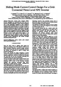
Fig. 1. Implementation results with Algorithm 3 and Algorithm 1 under state feedback-based ASMC with θ˜ = 4: Left column is for Algorithm 1 and right column is for Algorithm 3, where a: output tracking errors (radians) for joint 1, b: output tracking errors (radians) for joint 2, c: control input (newton-meters) for joint 1,and d: control input (newton-meters) for joint 2.

IV. D ESIGN S YNTHESIS AND I MPLEMENTATION R ESULTS This section presents the design and implementation process of the proposed technique on a 2-DOF robotic system [38]. The dynamic equation for this robot system can be defined as

m11 m21

m12 m22

q¨1 c + 11 q¨2 c21

c12 c22

q˙1 q˙2

=

τ1 τ2

(9)

with m11 = (θ1 + 2θ2 + 2θ2 cos q2 ), m12 = (θ2 + θ2 cos q2 ), m21 = (θ2 + θ2 cos q2 ), m22 = θ2 , c11 = −2q˙2 θ2 sin q2 , c12 = −q˙2 θ2 sin q2 , c21 = q˙1 θ2 sin q2 , c22 = 0, θ1 = m1 l2 , θ2 = m2 l2 , l is the link lengths and m1 and m2 in kg are the masses of link 1 and link 2, respectively. The robot operates in the horizontal plane so the gravitational force vector is G = 0. We now generate the reference trajectory, qd (t), for the given robot model to follow, a square wave with a period of 8 s and an amplitude of ± 1 radian is pre-filtered with a critically damped 2nd-order linear filter using a bandwidth of ωn = 2.0 rad/sec. Specifically, our main target is to use a desired trajectory that is usually used in industrial robotic systems. To design and implement proposed algorithms, let us first consider that the plant parameter θ ∈ 2 belongs to a known but comparatively large compact set as Ω ∈ [−10, 10]. We define the initial states as e(0) = 2 and eˆ(0) = 2. We also consider that the large initial estimation errors as θ˜1 (0) = 10 and θ˜2 (0) = 10. Then, we split the parameter set Ω equally into a finite number of smaller compact 41 subsets {Ω }, that is, Ω = as θi ∈ Ωi with Ω = 41 i i=1 i=1 {θi } = {−10, −9.5, ., ., ., ., ., ., ., ., 9.5, 10} × {−10, 10}. The control design parameters are chosen as λ1 = 2, λ2 = 2, K1 = 125, K2 = 125, Ki1 = 15, Ki2 = 15, φi1 = 0.7, φi2 = 0.7, and Γ = [Γ1 ; Γ2 ] with Γ1 = 10 and Γ2 = 10. Applying with the

Fig. 2. Implementation results with Algorithm 3 and Algorithm 1 with state feedback-based ASMC under θ˜ = 8: Left column is for Algorithm 1 and right column is for Algorithm 3, where a: output tracking errors (radians) for joint 1, b: output tracking errors (radians) for joint 2, c: control input (newton-meters) for joint 1, and d: control input (newton-meters) for joint 2.

above design constants, we then construct a family of candidate controllers as a state and output feedback as S i τ (e, Qd , θi ) = Sat Y (e, q˙r , q¨r )θi − KS − Ki sat φi Sˆ i e, Qd , θi ) = Y (ˆ e, qˆ˙ r , ¨qˆr )θi − KSˆ − Ki sat τ (ˆ φi with i = 41, respectively. Our first aim is to compare the tracking performance of the switching logic proposed in Algorithm 1 and Algorithm 3. For this purpose, we first assume that the position and velocity signals are available for feedback design. Then, we follow the switching steps derived in Algorithms 1 and 3 using the resetting condition V˙ (t) ≤ 0. The small time constant is considered for this test as td = 0.003. The implemented results are shown in Figs. 1 and 2 for the state feedback case with θ˜ = 4 and θ˜ = 8, that is, i∗ = 29 and i∗ = 37, respectively. The left


Fig. 3. Implementation results with Theorem 1 and Theorem 4 with θ˜ = 4: Left column is for Theorem 1 and right column is for Theorem 4, where a: output tracking errors (radians) for joint 1, b: output tracking errors (radians)for joint 2, c: control input (newton-meters) for joint 1, and d: control input (newton-meters) for joint 2.

column of each figure is for Algorithm 1, and the right column of each figure is for Algorithm 3. By comparing Figs. 1 and 2, one can observe that the tracking errors under switching Algorithm 1 are larger than the tracking errors under the logic introduced in Algorithm 3. Notice also from the left column of Figs. 1 and 2 that the transient tracking errors under the pre-routed switching-logic increase with the increase of i∗ . This is mainly because the switching has to scan through a number of candidate controllers before converging to the one that satisfies the Lyapunov inequality. As a result, relatively large transient tracking errors and control efforts under pre-routed switching approach can be seen during the transient phase. Such undesirable transient behavior of prerouted switching-logic can be reduced by using the switchinglogic proposed in Algorithm 2 and Algorithm 3. Now, we show that the performance obtained under state feedback-based design can be recovered by using output feedback design. To show that, our first task is to ensure the robust reconstruction of the unknown states by using linear observer. We compare the control performance of Theorem 1 with Theorem 4 (output feedback case) for two different observer speeds as = 0.005 (very high speed observer) and = 0.1 (slow speed observer). However, we keep the controller design parameters the same as used for the evaluation of the state feedback-based design. The two sets of the observer design parameters are considered for the evaluation as H1 = I2×2 , H2 = I2×2 , = 0.005 and H1 = 20I2×2 , H2 = 20I2×2 , = 0.1. Then, we define the small time constant td as td = 0.005 and the values of kf 1 and kf 2 as kf 1 = 0.05 and kf 2 = 0.05. With these designs parameters, let us implement the output feedback design proposed in Theorem 1 and Theorem 4 on the given system. The tested results are shown in Fig. 3–6. Figs. 3 and 4 show the tracking performance with the chosen estimation error as θ˜ = 4. Figs. 5 and 6 show the implementation results under θ˜ = 8. Figs. 3 and 4 show the control performance when observer design constants are chosen as H1 = I2×2 , H2 = I2×2 , and = 0.005. Figs. 5 and 6 show the tracking convergence with the following observer design constants,

2451

Fig. 4. Implementation results with Theorem 1 and Theorem 4 with θ˜ = 4: Left column is for Theorem 1 and right column is for Theorem 4, where a: black-dash line is for output tracking (radians) for joint 1, (black-solid line is for desired tracking), b: black-dash line is for output tracking (radians) for joint 2, black-solid line is for desired tracking, c: control input (newton-meters) for joint 1, and d: control input (newton-meters) for joint 2.

Fig. 5. Implementation results with Theorem 1 and Theorem 4 with θ˜ = 8: Left column is for Theorem 1 and right column is for Theorem 4, where a: black-dash line is for the output tracking (radians) for joint 1, black-solid line is for the desired tracking, b: black-dash line is for the output tracking (radians) for joint 2, black-solid line is for desired tracking), c: control input (newtonmeters) for joint 1, and d: control input (newton-meters) for joint 2.

Fig. 6. Implementation results with Theorem 3 and SM-based ASMC under θ˜ = 8: Left column is for ASMC (4) and right column is for Theorem 3, where a: output tracking errors (radians) for joint 1, b: output tracking errors (radians) for joint 2, c: control input (newton-meters) for joint 1, and d: control input (newton-meters) for joint 2.

2452


V. C ONCLUSION In this paper, we have proposed multiple parameters modelbased sliding mode technique to improve the tracking performance for a certain class of nonlinear mechanical systems. The design uses logic-based switching to identify an appropriate controller from the finite set of candidate state and output feedback controllers. The introduced method can be used to remove the chattering and infinitely fast switching control problem from the robust control strategy. The evaluation on a 2-DOF robotic system illustrates the theoretical development of the proposed distributed multiple-model-based SMC design. ACKNOWLEDGMENT

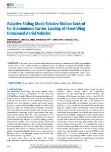
Fig. 7. Implementation results with Theorem 4 and SM-based AOFBSMC (5) under θ˜ = 8: Left column is for AOFBSMC (5) and right column is for Theorem 4, where a: output tracking errors (radians) for joint 1, b: output tracking errors (radians) for joint 2, c: control input (newton-meters) for joint 1, and d: control input (newton-meters) for joint 2.

The authors would like to thank the associate editor and the anonymous reviewers for their constructive comments, which greatly improved the quality of this work.

H1 = 20I2×2 , H2 = 20I2×2 , and = 0.1. The left column of each figure is for Theorem 1 and the right column of each figure is for Theorem 4. In view of Figs. 3–6, one can notice that the performance achieved under output feedback design recovers the performance achieved under state feedback design. However, undesirable transient tracking and control oscillation under state and output feedback-based pre-routed switchinglogic with Algorithm 1 are clearly observed (see left column of each figure). Let us now compare the tracking performance of Theorems 3 and 4 with the SM-based adaptive SMC algorithms (4) and (5). The tested results are shown in Fig. 6 with θ˜ = 8 (right column is for Theorem 3 and left column is for the SM-based ASMC (4)). The control parameters for SM-based ASMC design are chosen as λ1 = 2, λ2 = 2, K1 = 125, K2 = 125, K1 = 15, K2 = 15, φ1 = 0.7, φ2 = 0.7, Γ = [Γ1 0; 0 Γ2 ] with Γ1 = 100 and Γ2 = 100. The constants for multimodelbased ASMC design are considered as λ1 = 2, λ2 = 2, K1 = 125, K2 = 125, Ki1 = 15, Ki2 = 15, φi1 = 0.7, φi2 = 0.7, Γ = [Γ1 0; 0 Γ2 ] with Γ1 = 10 and Γ2 = 10. By comparing the left and right columns of Fig. 6, we can observe that the tracking errors under Lyapunov-based switching almost closed to zero, but relatively large tracking errors can be noticed under a single model-based ASMC algorithm. We now compare the tracking performance of Theorem 4 with the single modelbased AOFBSMC algorithm defined by (5). The conducted results are shown in Fig. 7 under θ˜ = 8 (i∗ = 37) with the following design constants: H1 = 20I2×2 , H2 = 20I2×2 , = 0.1, kf 1 = 0.05, kf 2 = 0.05, and td = 0.005. For fair comparison, we keep the same set of controller design parameters as used for our previous evaluation. In view of the left (SM-based AOFBSMC design) and the right column (Theorem 4) of Fig. 7, we can see that the output tracking under Theorem 4 converges to the desired one, but quite a large tracking error can be seen under the single model-based AOFBSMC approach. In view of the left (SM-based AOFBSMC design) and the right column (Theorem 4) of Fig. 7, we can see that the output tracking under Theorem 4 converges to the desired one, but quite a large tracking error can be seen under the single model-based AOFBSMC approach.

[1] A. Rojko and K. Jezernik, “Sliding-mode motion controller with adaptive fuzzy disturbance estimation,” IEEE Trans. Ind. Electron., vol. 51, no. 5, pp. 963–971, Oct. 2004. [2] A. S. Morse, “Supervisory control of families of linear set-point controllers—Part I,” IEEE Trans. Autom. Control, vol. 41, no. 10, pp. 1413–1431, Oct. 1996. [3] A. Tayebi and S. Islam, “Experimental evaluation of an adaptive iterative learning control scheme on a 5-DOF robot manipulators,” in Proc. IEEE Int. Conf. Control Appl., Taipei, Taiwan, Sep. 2–4, 2004, pp. 1007–1011. [4] A. Tayebi and S. Islam, “Adaptive iterative learning control for robot manipulators: Experimental results,” Control Eng. Pract., vol. 14, no. 7, pp. 843–851, Jul. 2006. [5] A. V. Topalov and O. Kaynak, “On line learning in adaptive neurocontrol for compliance tasks of robotic manipulators,” IEEE Trans. Syst., Man, Cybern., vol. 31, no. 3, pp. 445–450, Jun. 2001. [6] C. Canudas De Wit and N. Fixot, “Adaptive control of robot manipulators via velocity estimated feedback,” IEEE Trans. Autom. Control, vol. 37, no. 8, pp. 1234–1237, Aug. 1992. [7] H. Schwartz and S. Islam, “An evaluation of adaptive robot control via velocity estimated feedback,” in Proc. Int. Conf. Control Appl., Montreal, QC, Canada, May 30–Jun. 1, 2007, pp. 325–333. [8] C. Hua, X. Guan, and G. Duan, “Variable structure adaptive fuzzy control for a class of nonlinear time delay systems,” Fuzzy Sets Syst., vol. 148, no. 3, pp. 453–468, Dec. 2004. [9] C.-J. Lin, “Variable structure model following control of robot manipulators with high-gain observer,” JSME Int. J. Ser. C, vol. 47, no. 2, pp. 591– 600, 2004. [10] C. Y. Su, T. P. Leung, and Q. J. Zhou, “A novel variable structure control scheme for robot trajectory control,” in Proc. IFAC Triennial World Congr., 1990, vol. 5, pp. 117–120. [11] D. Angeli and E. Mosca, “Lyapunov-based switching supervisory control of nonlinear uncertain systems,” IEEE Trans. Autom. Control, vol. 47, no. 3, pp. 500–505, Mar. 2002. [12] E. S. Shin and K. W. Lee, “Robust output feedback control of robot manipulators using high-gain observer,” in Proc. IEEE Int. Conf. Control Appl., 1999, pp. 881–886. [13] H. Asada and J. J. Slotine, Robot Analysis and Control. New York: Wiley, 1986. [14] H. Hashimoto, K. Maruyama, and F. Harashima, “A microprocessor-based robot manipulator control with sliding mode,” IEEE Trans. Ind. Electron., vol. IE-34, no. 1, pp. 11–18, Feb. 1987. [15] B. Bandyopadhyay, P. S. Gandhi, and S. Kurode, “Sliding mode observer based sliding mode controller for slosh-free motion through PID scheme,” IEEE Trans. Ind. Electron., vol. 56, no. 9, pp. 3432–3442, Sep. 2009. [16] K. C. Veluvolu and Y. C. Soh, “High-gain observers with sliding mode for state and unknown input estimations,” IEEE Trans. Ind. Electron., vol. 56, no. 9, pp. 3386–3393, Sep. 2009. [17] J. M. A.-D. Silva, C. Edwards, and S. K. Spurgeon, “Sliding-mode outputfeedback control based on LMIs for plants with mismatched uncertainties,” IEEE Trans. Ind. Electron., vol. 56, no. 9, pp. 3675–3683, Sep. 2009.

R EFERENCES


[18] C. Lascu, I. Boldea, and F. Blaabjerg, “A class of speed-sensorless slidingmode observers for high-performance induction motor drives,” IEEE Trans. Ind. Electron., vol. 56, no. 9, pp. 3394–3403, Sep. 2009. [19] J. J. E. Slotine and S. S. Sastry, “Tracking control of nonlinear system using sliding surface, with application to robot manipulators,” Int. J. Control, vol. 38, no. 2, pp. 465–492, Aug. 1983. [20] J. Y. Hung, W. Gao, and J. C. Hung, “Variable structure control: A survey,” IEEE Trans. Ind. Electron., vol. 40, no. 1, pp. 2–22, Feb. 1993. [21] K. D. Young, “Controller design for robot a manipulator using theory of variable structure control,” IEEE Trans. Syst., Man, Cybern., vol. SMC-8, no. 2, pp. 101–109, Feb. 1978. [22] K. Erbatur, O. Kaynak, and A. Sabanovic, “A study on robustness property of sliding mode controllers: A novel design and experimental investigations,” IEEE Trans. Ind. Electron., vol. 46, no. 5, pp. 1012–1018, Oct. 1999. [23] K. Erbatur, O. Kaynak, and A. Sabanovic, “Robust control of a direct drive manipulator,” in Proc. IEEE ISIC/CIRA/ASAS Joint Conf., Gaithersburg, MD, Sep. 14–17, 1998, pp. 108–113. [24] K. J. Astrom and B. Wittenmark, Adaptive Control, 2nd ed. Reading, MA: Addison-Wesley, 1995. [25] X. R. Han, E. Fridman, S. K. Spurgeon, and C. Edwards, “On the design of sliding-mode static-output-feedback controllers for systems with state delay,” IEEE Trans. Ind. Electron., vol. 56, no. 9, pp. 3656–3664, Sep. 2009. [26] L. C. Fu and T. L. Liao, “Globally stable robust tracking of nonlinear system using variable structure control and application to a robot manipulator,” IEEE Trans. Autom. Control, vol. 35, no. 12, pp. 1345–1350, Dec. 1990. [27] M. Akar, “Robust tracking for a class of nonlinear systems using multiple models and switching,” in Proc. Amer. Control Conf., Portland, OR, 2005, pp. 4056–4061. [28] M. Erlic and W. Lu, “A reduced-order adaptive velocity observer for manipulator control,” IEEE Trans. Robot. Autom., vol. 11, no. 2, pp. 293– 303, Apr. 1995. [29] M. L. Corradini, T. Leo, and G. Orlando, “Robust stabilization of a class of nonlinear systems via multiple model sliding mode control,” in Proc. Amer. Control Conf., Chicago, IL, Jun. 2000, pp. 631–635. [30] M. L. Corradini and G. Orlando, “Transient improvement of variable structure controlled systems via multimodel switching control,” Trans. ASME, J. Dyn. Syst. Meas. Control, vol. 124, no. 2, pp. 321–326, Jun. 2002. [31] T. M. R. Akbarzadeh and R. Shahnazi, “Direct adaptive fuzzy PI sliding mode control for a class of uncertain nonlinear systems,” in Proc. IEEE Int. Conf. Syst., Man, Cybern., 2005, vol. 3, pp. 2548–2553. [32] M. S. Branicky, “Multiple Lyapunov functions and other analysis tools for switched and hybrid systems,” IEEE Trans. Autom. Control, vol. 43, no. 4, pp. 475–482, Apr. 1998. [33] M. S. De Queiroz, J. Hu, D. Dawson, T. Burg, and S. Donepudi, “Adaptive position/force control of robot manipulators without velocity measurements: Theory and experimentation,” IEEE Trans. Syst., Man, Cybern. B, Cybern., vol. 27, no. 5, pp. 796–809, Sep. 1997. [34] M. W. Spong and M. Vidyasagar, Robot Dynamics and Control. New York: Wiley, 1989. [35] P. R. Pagilla and M. Tomizuka, “An adaptive output feedback controller for robot arms: Stability and experiments,” Automatica, vol. 37, no. 7, pp. 983–995, Jul. 2001. [36] Q.-H. Meng and W.-S. Lu, “A unified approach to stable adaptive force/position control of robot manipulators,” in Proc. Amer. Control Conf., Jun. 1994, pp. 200–201. [37] R. Martinez and J. Alvarez, “Hybrid sliding-mode-based control of underactuated system with dry friction,” IEEE Trans. Ind. Electron., vol. 55, no. 11, pp. 3998–4003, Nov. 2008. [38] S. Islam, “Adaptive output feedback for robot manipulators using linear observer,” in Proc. Int. Conf. Intell. Syst. Control, Orlando, FL, Nov. 16–18, 2008, pp. 38–43. [39] S. Lim, D. Dawson, and K. Anderson, “Re-examining the Nicosia–Tomei robot observer-controller from a backstepping perspective,” IEEE Trans. Control Syst. Technol., vol. 4, no. 3, pp. 304–310, May 1996. [40] S. Nicosia and P. Tomei, “Robot control by using only joint position measurements,” IEEE Trans. Autom. Control, vol. 35, no. 9, pp. 1058– 1061, Sep. 1990. [41] V. I. Utkin, “Variable structure systems with sliding mode,” IEEE Trans. Autom. Control, vol. AC-22, no. 2, pp. 212–222, Apr. 1977. [42] W. Chen and M. Saif, “Output feedback controller design for a class of MIMO nonlinear systems using high-order sliding-mode differentiators with application to a laboratory 3-D crane,” IEEE Trans. Ind. Electron., vol. 55, no. 11, pp. 3985–3997, Nov. 2008.

2453

[43] W. E. Dixon, M. S. Queiroz, F. Zhang, and D. M. Dawson, “Tracking control of robot manipulators with bounded torque inputs,” Robotica, vol. 17, no. 2, pp. 121–129, Mar. 1999. [44] W.-S. Lu and Q.-H. Meng, “Regressor formulation of robot dynamics: Computation and applications,” IEEE Trans. Robot. Autom., vol. 9, no. 3, pp. 323–333, Jun. 1993. [45] X.-G. Yan and C. Edwards, “Adaptive sliding-mode-observer-based fault reconstruction for nonlinear systems with parametric uncertainties,” IEEE Trans. Ind. Electron., vol. 55, no. 11, pp. 4029–4036, Nov. 2008. [46] J.-B. Pomet and L. Praly, “Adaptive nonlinear regulation estimation from the Lyapunov equation,” IEEE Trans. Autom. Control, vol. 37, no. 6, pp. 729–740, Jun. 1992.

Shafiqul Islam (SM’04–M’10) received the B.Sc. degree in electrical and electronic engineering from Chittagong University of Engineering and Technology, Chittagong, Bangladesh, in 1998, and the M.Sc. degree in control engineering from Lakehead University, Thunder Bay, ON, Canada, in 2004. From 1999 to 2001, he was a full-time Lecturer and an Assistant Professor in the Department of Electrical and Electronic Engineering, Chittagong University of Engineering and Technology. From 2002 to 2007, he was on leave from the Chittagong University of Engineering and Technology at Lakehead University and at Carleton University, Ottawa, ON, Canada. He is currently with the Department of Systems and Computer Engineering, Carleton University. His research interests include dynamics and control of mechatronic and robotic systems, hybrid and intelligent systems, medical mechatronic, bilateral telemanipulations over the Internet, and haptics with medical applications. Mr. Islam was the recipient of the 2009–2010 Research Excellence Award from Carleton University, Canada, for outstanding graduate research work in science and engineering. Mr. Islam also received the Natural Science and Engineering Research Council (NSERC) of Canada Postdoctoral Fellowship Grant for visiting research laboratory.

Xiaoping P. Liu (M’02–SM’07) received the Ph.D. degree from the University of Alberta, Edmonton, Canada, in 2002. He has been with the Department of Systems and Computer Engineering, Carleton University, Ottawa, ON, Canada since July 2002, and he is currently a Canada Research Chair. He has published more than 150 research articles and serves as an Associate Editor for several journals, including IEEE/ASME Transactions on Mechatronics and IEEE Transactions on Automation Science and Engineering. Dr. Liu is a licensed Member of the Professional Engineers of Ontario (P.Eng) and a senior member of the IEEE. He received a 2007 Carleton Research Achievement Award, a 2006 Province of Ontario Early Researcher Award, a 2006 Carty Research Fellowship, the Best Conference Paper Award of the 2006 IEEE International Conference on Mechatronics and Automation, and a 2003 Province of Ontario Distinguished Researcher Award.