Robust Solutions of Conic Quadratic Problems

Robust Solutions of Conic Quadratic Problems research thesis

Submitted in Partial Fulfillment of the Requirements for the Degree of Doctor of Philosophy

Odellia Boni

Submitted to the Senate of the Technion - Israel Institute of Technology

Sivan 5766

Haifa

June 2006

The Research Thesis Was Done Under The Supervision of Professor Aharon Ben-Tal in The Faculty of Industrial Engineering and Management.

THE GENEROUS FINANCIAL HELP OF THE TECHNION IS GRATEFULLY ACKNOWLEDGED.

I would like to thank Prof. Ben-Tal and Prof. Nemirovski for their guidance and quick response in every issue.

Special thanks are attributed to Dr. Amir Beck for his help and constructive remarks.

The listening ear and helping hand of the IE&M faculty academic staff, administrative staff and students are highly appreciated.

And last but certainly not least, I am grateful for the support of my wonderful family and friends.

Contents 1 Abstract

1

2 Introduction 2.1 Robust Optimization . . . . . . . . . . . . . . . . . . . . . . . . . . . . . 2.2 Set inclusion uncertainty . . . . . . . . . . . . . . . . . . . . . . . . . . . 2.2.1 Robust counterpart of a linear constraint . . . . . . . . . . . . . . 2.2.2 Robust counterpart of a conic quadratic constraint . . . . . . . . 2.2.3 A semidefinite constraint . . . . . . . . . . . . . . . . . . . . . . . 2.2.4 Approximate robust counterpart . . . . . . . . . . . . . . . . . . . 2.2.5 Approximate robust counterpart for a conic quadratic constraint . 2.2.6 Approximate robust counterpart for a semidefinite constraint . . . 2.2.7 Other robust counterparts for conic constraints . . . . . . . . . . 2.3 Probabilistic uncertainty . . . . . . . . . . . . . . . . . . . . . . . . . . . 2.3.1 Approximate robust counterpart . . . . . . . . . . . . . . . . . . . 2.3.2 Exponential bounds on probabilities of large deviations in normed spaces . . . . . . . . . . . . . . . . . . . . . . . . . . . . . . . . . 2.3.3 A chance constraint of a linear constraint . . . . . . . . . . . . . . 2.3.4 A chance constraint of a conic quadratic constraint . . . . . . . . 2.3.5 A chance constraint of a semidefinite constraint . . . . . . . . . . 2.3.6 Other counterparts for conic chance constraints . . . . . . . . . . 2.4 Adjustable variables . . . . . . . . . . . . . . . . . . . . . . . . . . . . . 2.4.1 Affinely adjustable robust counterpart . . . . . . . . . . . . . . . 2.4.2 Affinely adjustable robust counterpart of a linear constraint . . .

. . . . . . . . . . .

3 3 4 5 6 8 8 9 10 12 13 13

. . . . . . . .

14 15 16 17 18 19 20 20

3 Research goals 23 3.1 Robust counterpart of a conic quadratic constraint . . . . . . . . . . . . . 23 3.2 Adjustable robust counterpart for conic constraints . . . . . . . . . . . . . 24 3.3 Mixed uncertainty . . . . . . . . . . . . . . . . . . . . . . . . . . . . . . . 24 4 Approximate robust counterpart of set inclusion uncertainty 4.1 An example: implementation errors 4.2 An example: the portfolio problem 4.2.1 Factor models . . . . . . . . 82

a conic quadratic constraint with 25 . . . . . . . . . . . . . . . . . . . . . . 27 . . . . . . . . . . . . . . . . . . . . . . 28 . . . . . . . . . . . . . . . . . . . . . . 30

4.3

An example : the stable grasp problem . . . . . . . . . . . . . . . . . . . . 32

5 Affinely adjustable robust counterpart of conic constraints 5.1 Affinely adjustable robust counterpart of a conic quadratic constraint 5.1.1 Fixed Recourse . . . . . . . . . . . . . . . . . . . . . . . . . . 5.1.2 Variable Recourse . . . . . . . . . . . . . . . . . . . . . . . . . 5.1.3 An example: subway route design . . . . . . . . . . . . . . . . 5.1.4 An example: retailer-supplier flexible commitments contracts . 5.2 Affinely adjustable robust counterpart of a semidefinite constraint . . 5.2.1 Fixed Recourse . . . . . . . . . . . . . . . . . . . . . . . . . . 5.2.2 Variable Recourse . . . . . . . . . . . . . . . . . . . . . . . . .

. . . . . . . .

. . . . . . . .

. . . . . . . .

41 42 43 44 48 52 58 58 59

6 Mixed Uncertainty 6.1 Mixed uncertainty in a linear constraint . . . . . . . . 6.2 Mixed uncertainty in a conic quadratic constraint . . . 6.2.1 One-sided uncertainty . . . . . . . . . . . . . . 6.2.2 Two-sided uncertainty . . . . . . . . . . . . . . 6.3 Mixed uncertainty in a semidefinite constraint . . . . . 6.4 Other robust counterparts for mixed uncertainty model

. . . . . .

. . . . . .

. . . . . .

63 64 65 66 68 72 73

7 Discussion and Conclusions

. . . . . .

. . . . . .

. . . . . .

. . . . . .

. . . . . .

. . . . . .

. . . . . .

. . . . . .

76

List of Figures 4.1 4.2 4.3 4.4 4.5

4.6 4.7

4.8

4.9

5.1

5.2 5.3

Minimal VaR vs. uncertainty magnitude for nominal and robust portfolios. Confidence level: 95% . . . . . . . . . . . . . . . . . . . . . . . . . . . . . Relative difference in the VaR of the approximate robust portfolio and the worst-case VaR of the nominal portfolio vs. uncertainty magnitude . . . . A cylinder held by 3 symmetrically positioned robot fingers. . . . . . . . . Maximal cylinder mass vs. perturbations magnitude (box uncertainty set) Relative error in maximal cylinder mass (between the approximate robust counterpart and the worst-case certain problem) vs. perturbations magnitude (box uncertainty set) . . . . . . . . . . . . . . . . . . . . . . . . . . . Maximal cylinder mass vs. perturbations magnitude (ellipsoidal uncertainty set) . . . . . . . . . . . . . . . . . . . . . . . . . . . . . . . . . . . . Relative error in maximal cylinder mass (between the approximate robust counterpart and the worst-case certain problem) vs. perturbations magnitude (ellipsoidal uncertainty set) . . . . . . . . . . . . . . . . . . . . . . . . Maximal cylinder mass calculated based on the approximate robust counterparts of Boni and Bertsimas and Sim vs. perturbations magnitude (ellipsoidal uncertainty set) . . . . . . . . . . . . . . . . . . . . . . . . . . . . Relative difference in maximal cylinder mass (between the approximate robust counterparts of Boni and Bertsimas and Sim) vs. perturbations magnitude (ellipsoidal uncertainty set) . . . . . . . . . . . . . . . . . . . .

32 33 35 36

37 38

39

39

40

Neighbourhoods (marked by grey squares) and subway stations locations (marked by rings) in the case of no implemetations error (ξ = 0), and for a randomly chosen implementation errors vector (ξ 6= 0). . . . . . . . . . . 51 Minimal total tunnels length vs. uncertainty magnitude. . . . . . . . . . . 52 Relative difference in minimal tunnels length between usual and affinely adjustable robust solutions vs. uncertainty magnitude. . . . . . . . . . . . 53

List of Tables 2.1

2.2 5.1

5.2

The form of the robust counterparts of conic constraints with structured uncertainty for various perturbations sets. LP, SOCP and SDP stand for linear, conic quadratic and semidefinite constraints, respectively. . . . . . . 12 functions and data corresponding to special conic constraints . . . . . . . . 12 The mean and standard deviation of the retailer’s cost in flexible commitments contract for ideal and robust solutions. The demands vary in an interval uncertainty of the size 2ρ. . . . . . . . . . . . . . . . . . . . . . . . 57 The mean and standard deviation of the retailer’s expenses in flexible commitments contract for ideal and affinely adjustable robust solutions. The demands vary in an interval uncertainty of the size 2ρ. . . . . . . . . . . . 58

Chapter 1 Abstract Optimization has become a leading methodology in many fields in recent years. However, a need to deal with uncertain data arose when optimization results were incorporated into real life applications. Robust optimization aims to find an optimal (or near optimal) solution which is feasible for every possible realization of the uncertain data. This work investigates robust optimization in three different aspects. The first is finding robust solutions to conic quadratic (SOCP) problems. Those are problems containing constraints of the form kAx + bk2 ≤ cT x + d where x is a vector of the decision variables and A,b,c,d are the (perhaps uncertain) data. The results known so far regarding such problems assumed that the uncertain data lies only in one side of the conic quadratic constraint or that the uncertainties which lie in the different sides of the constraint are independent. These are, of course, quite limiting assumptions. In this work we present conic quadratic problems with implementation errors and the portfolio and stable grasp problems for which these assumptions are inherently not true. We prove a new theorem which allows to relieve the independency assumption and find approximate robust solutions to these problems. Comparing the results to the exact robust solution (if we can find it) or bounds on it, we see that the relative error of the approximation is less than 9% for uncertainties as large as 10%. A comparison of our results with a very recent paper by Bertsimas and Sim, introducing an approximate robust counterpart to conic optimization problems (and amongst them to conic quadratic problems without assuming independency of the uncertainties affecting both sides of the conic quadratic constraints), reveals that our theorem yields a better approximation. The second part of this work deals with the adjustable variables approach. This approach can be exercised when part of the decision variables can be determined after some of the uncertain data has already realized. Such variables are called the adjustable variables. This approach was already incorporated into uncertain linear problems, but not to other types of optimization problems. In this work we prove a new result which incorporates the adjustable variables approach into robust conic quadratic and semidefinite optimization. Adjustable robust solutions to the problems of subway route design with implementation errors and retailer-supplier flexible commitments contracts facing uncertain demands are obtained using these results. Comparison of the adjustable solution with the nominal and non-adjustable robust solutions shows that the adjustable robust 1

solution maintains feasibility for all possible realizations, while being less conservative than the non-adjustable robust solution. In the third part of the work we present a model of mixed uncertainty, meaning, we look into cases where the uncertain data of the optimization problems is affected by bounded perturbations as well as random ones. In these cases we wish to ensure feasibility of the robust solution for all bounded perturbations and for the most probable random perturbations. We formulate tractable robust counterparts (or their approximations) for linear, conic quadratic and semidefinite constraints affected by both bounded and probabilistic uncertainties.

2

Chapter 2 Introduction 2.1

Robust Optimization

In recent years optimization became a leading methodology in engineering and control design. Most applications assume complete knowledge of the data of the optimization problem. However, often rises a need to solve uncertain optimization problems. There are several sources for the uncertainty: the data of the problem is not exactly known or cannot be exactly measured, or the exact solution of the problem cannot be implemented due to inherent inaccuracy of the devices. The data uncertainty results in uncertain constraints and objective function. There are cases in reality where, in spite of the data uncertainty, the solution must satisfy the actual constraints, for all (or most) possible realizations of the data. Such a solution is called a robust feasible solution. The problem of finding an optimal robust solution is called the robust counterpart of the original problem. It is, in fact, the problem of minimizing the objective function over the set of robust feasible solutions. In this work, we concentrate on conic optimization problems. An uncertain conic problem has the form min {cT x :

x∈ Rn

Aj x + bj ∈ Kj ,

j = 1 . . . N}

where Kj , j = 1, . . . , N are closed, pointed, non-empty, convex cones. We may assume, without loss of generality, that the objective function is certain, and only the data Aj , bj is uncertain. We distinguish between two types of uncertainty: 1. Set inclusion uncertainty where the data is only known to belong to some bounded uncertainty sets Uj , (Aj , bj ) ∈ Uj

j = 1 . . . N.

2. Probabilistic uncertainty where the uncertain parameters are random vectors belonging to some set of probability distribution functions.

3

In this work we will assume that the uncertainty is structured meaning: Uj = {(Aj , bj ) = (A0j , b0j ) + ρ

L X

ζ` (A`j , b`j ) :

ζ ∈ Vj },

(2.1)

`=1

where (A0j , b0j ) are the nominal values of the uncertain parameters, (A`j , b`j ) is the `-th perturbation direction, ζ ∈ RL is a perturbations vector, ρ > 0 is a parameter expressing the magnitude of the perturbations and Vj is the perturbations set. Furthermore, we assume that the uncertainty affecting the problem is a cartesian product of the uncertainties affecting each constraint. Meaning, the uncertainties affecting each constraint is independent of each other. Hence, the crucial step in building a robust counterpart for a given problem is the ability to build a robust counterpart for a single constraint. Therefore, in what follows we drop the index j. When the problem has additional convex certain constraints, it suffices to add these constraints to the corresponding robust counterpart formulation. The most common types of conic constraints are: n 1. linear: K = R+

2. conic quadratic: K = {(x, t) : x ∈ Rn , t ≥ 0, kxk2 ≤ t} 3. semidefinite: K = {X ∈ S m : X º 0} (S m is the subspace of m × m symmetric matrices) The robust counterpart of a certain conic constraint typically does not maintain the original conic structure. Its structure depends on the geometry/probability distribution of the uncertainty set. In the following, we will try to summarize the research done so far in finding tractable robust counterparts of conic constraints.

2.2

Set inclusion uncertainty

When the data uncertainty is bounded, we are looking for solutions which are feasible for any realization of the data. Thus, we are looking for the set of solutions x ∈ Rn of the semi-infinite inequality system A[ρζ]x + b[ρζ] ≥K 0,

∀ζ ∈ V,

(2.2)

where the notation a ≥K 0 means a ∈ K and the notation a[z] means that a depends affinely on z. Equation (2.2) is equivalent to: inf A[ρζ]x + b[ρζ] ≥K 0.

ζ∈V

4

Thus, the robust counterpart of the original constraint in the case of bounded uncertainty takes into account the worst case scenario. Note that there are situations in reality where we are willing to overlook rare events, and in these situations this approach may be too conservative. On the other hand, it may well happen that ensuring robust feasibility is nearly costless, meaning the difference in the optimal objective function values of the original problem and its robust counterpart is small [2],[3],[4]. The work that has been done so far has concentrated on several types of uncertainty sets, most of them can be formulated as an intersection of ellipsoids with a common center, meaning: V = {ζ ∈ RL :

ζ T Qk ζ ≤ 1,

with Qk º 0 and

K X

k = 1, . . . , K},

Qk  0.

(2.3)

(2.4)

k=1

The form (2.3) includes two important special cases: • simple ellipsoidal uncertainty (K = 1); • box uncertainty (K = L, {Qk }kk = 1 and {Qk }ij = 0 (i 6= k or j 6= k) for k = 1 . . . K). A more general uncertainty set is a semidefinite representable (SDR) set, i.e., a set which can be represented as the projection of a set described by a linear matrix inequality (LMI): V = {ζ ∈ RL :

L X

∃u ∈ RS ,

ζ` P` +

`=1

S X

us Fs − T º 0}

(2.5)

s=1

where T , P` (` = 1 . . . L) and Fs (s = 1 . . . S) are given symmetric matrices. It is well known that SDR-sets include intersection of ellipsoids and many more [7].

2.2.1

Robust counterpart of a linear constraint

A linear constraint is of the form: aT x + b ≥ 0

(2.6)

where a ∈ Rn , b ∈ R are the parameters of the constraint. In the case of unstructured box uncertainty, the robust counterpart of (2.6) is a set of linear constraints [1], [3]. In the case where the uncertainty set is structured and the perturbations set is an intersection of ellipsoids, the robust counterpart is an explicit conic quadratic program:

5

Theorem 2.2.1 Consider the linear constraint (2.6) with structured uncertainty (2.1) where the perturbations set has the form (2.3) and (2.4). Then, x satisfies (2.6) for all possible perturbations in this set, if and only if there exists τk ∈ R, µk ∈ RL , k = 1, . . . , K such that (x, τ, µ) satisfies: P

(a0 )T x + b0 − ρ K k=1 τk ≥ 0   1 T (a ) x + b1 1   PK .. 2   Q . k=1 k µk =   (aL )T x + bL kµk k2 ≤ τk k = 1, . . . , K The proof is based on strong duality theorem for conic problems [1]. In the case where the uncertainty set is structured and the perturbations set is semidefinite representable, the robust counterpart is a semidefinite program: Theorem 2.2.2 Consider the linear constraint (2.6) with structured uncertainty (2.1) where the perturbations set is bounded, including zero and semidefinite representable, meaning, has the form (2.5). Assume in addition that ¯ u¯) : ∃(ζ,

R X

ζ¯r Pr +

r=1

S X

u¯s Fs  T.

s=1

Then, x satisfies (2.6) for all possible perturbations if and only if, there exists a symmetric matrix V such that the triple (x, τ, V ) satisfies: ((a0 )T x + b0 ) + T r(T V ) T r(V P` ) T r(V Fs ) V

≥ = = º

τ, ρ((a` )T x + b` ) ` = 1 . . . L, 0 s = 1 . . . S, 0.

The proof is based on strong duality theorem for conic problems and can be found in [1],[8],[12].

2.2.2

Robust counterpart of a conic quadratic constraint

Conic quadratic inequality is of the form: kAx + bk2 ≤ cT x + d,

(2.7)

where A ∈ Rm×n , b ∈ Rm , c ∈ Rn , d ∈ R being the constraint parameters. We begin by considering a conic quadratic constraint of the form kAx + bk2 ≤ τ, 6

(2.8)

where the uncertainty lies only on the left hand side of the constraint, that is, only the parameters A and b are uncertain. We will call such a constraint a one-sided conic quadratic constraint. This type of constraint occurs, for example, in least square fit problems. These are problems of finding a solution x to an overdetermined set of equations Ax ' b, which minimizes the data error kAx − bk. El Ghaoui and Lebret [6] analyzed the robustness of least square problems for two types of uncertainty sets. The first is unstructured norm bounded uncertainty set. They showed that in this case the robust counterpart can be formulated as a conic quadratic problem. The second uncertainty set considered by El Ghaoui and Lebret was structured uncertainty with a unit ball perturbations set, and their results are a special case of the result described in Theorem 2.2.3 below. Ben-Tal and Nemirovski considered a one sided conic quadratic constraint (2.8) with structured uncertainty. They found that when the perturbation set is a simple ellipsoid the robust counterpart is given by a single LMI [9]: Theorem 2.2.3 Consider the constraint (2.8) where the parameters A, b have structured uncertainty (2.1) and the perturbations set is given by (2.3) and (2.4) with K = 1. Then a pair (x, τ ) satisfies (2.8) for all possible perturbations if and only if there exists a scalar λ1 ≥ 0 such that the triple (x, τ, λ1 ) satisfies the following LMI: 



τ − λ1 0 a[x]T  0 λ1 Q1 ρA[x]T   º0 a[x] ρA[x] τ IM where a[x] = A0 x + b0 A[x] = (A1 x + b1 , . . . , AL x + bL )

(2.9) (2.10)

Ben-Tal and Nemirovski also proved that for a perturbation set which is an intersection of several ellipsoids the verification of (2.8) for all possible perturbations is an NP-hard problem [9]. Ben-Tal and Nemirovski used the above mentioned theorems to handle the situation where the uncertainty affecting the conic quadratic constraint (2.7) is structured and sidewise, i.e., the uncertainty affecting the right hand side in (2.7) is independent of the one affecting the left hand side. More specifically, the uncertainty set U can be represented as U = U L × U R, where (A, b) ∈ U L , (c, d) ∈ U R . The side-wise uncertainty assumption implies the following fact: 7

x is robust feasible for (2.7) if and only if there exists τ ∈ R such that: kAx − bk2 ≤ τ, ∀A, b ∈ U L , τ ≤ cT x + d, ∀c, d ∈ U R .

(2.11) (2.12)

This fact allows handling (2.7) by treating separately (2.11) and (2.12). (2.12) is an uncertain linear constraint and has a robust counterpart in the cases of intersection of ellipsoids and semidefinite representable perturbation sets. (2.11) is a one-sided conic quadratic constraint and has a robust counterpart in the case of simple ellipsoidal perturbation set. Combining these robust counterparts yields a robust counterpart to conic quadratic constraint with side-wise uncertainty.

2.2.3

A semidefinite constraint

A semidefinite constraint is of the form: B+

n X

xi Ai º 0

(2.13)

i=1

with B, A1 , . . . , An ∈ S m being the parameters of the constraint. Finding a robust counterpart in the case of structured uncertainty with an ellipsoidal perturbations set is an NP-hard problem [9].

2.2.4

Approximate robust counterpart

For robust optimization to be an applicable methodology for real life large scale problems, it is essential that the robust counterpart be computationally tractable, meaning solvable in polynomial time with respect to the problem size. Tractability of the robust counterpart depends on the original optimization problem and the uncertainty set we consider. In many cases, the robust counterpart is not tractable, e.g. verifying (2.2) is an NP-hard problem. Therefore, arises the need to find an approximation to the robust counterpart and to estimate its quality. Ben-Tal and Nemirovski [9] defined a tractable approximation for the robust counterpart as a system S = Sρ (x, u) of explicit convex constraints on x and additional variables u such that Rρ ⊆ Xρ , where Rρ = {x : ∃u : (x, u) satisfies Sρ (x, u)}, Xρ = {x : x satisfies (2.2)}. Thus, the possibility to augment a given x to a solution to S implies that x satisfies (2.2). In addition, it is required that building S, given ρ and the data A, b, be in time polynomial in the size of these data. Since Rρ is convex, one can minimize convex objectives over x’s in this set which also satisfy, perhaps, additional explicit convex constraints. 8

Level of conservativeness The proximity of Rρ to Xρ is called level of conservativeness and is defined by: ρ∗ = min {α :

Xαρ ⊆ Rρ ⊆ Xρ }

α>1

This definition exploits the obvious fact that the set of robust feasible solutions Xρ , shrinks as the perturbations magnitude increases. If the perturbations magnitude is larger than the level of conservativeness, then the set of robust feasible solutions is no longer included in Rρ . Hence, the level of conservativeness actually measures the proximity of Xρ to Rρ . The smaller the level of conservativeness is, the better the approximation. In reality the uncertainty magnitude, ρ, is usually given by order of magnitude, so if the level of conservativeness is close to 1, the approximate robust counterpart can be viewed, for all practical purposes, as the exact robust counterpart.

2.2.5

Approximate robust counterpart for a conic quadratic constraint

As was mentioned before, finding the set of robust feasible solutions of a one-sided conic quadratic constraint with structured uncertainty and a perturbations set which is an intersection of several ellipsoids is an NP-hard problem [9]. However, the following theorem by Ben-Tal and Nemirovski [8], [12] gives an approximate robust counterpart which is an explicit semidefinite program. Theorem 2.2.4 Consider the constraint (2.8) where the parameters A, b have structured uncertainty (2.1) and the perturbations set is given by (2.3) and (2.4) with K > 1. Then a pair (x, τ ) satisfies (2.8) for all possible perturbations if there exists λ ∈ RK such that the set (x, τ, λ) satisfies:   

τ−

P k

0 a[x]

λk



0 a[x]T P T  k λk Qk ρA[x]  º 0, ρA[x] τ IM

λ ≥ 0,

with a[x] and A[x] as given by (2.9)–(2.10) An upper bound on the level of conservativeness of the approximation is given by the following theorem: Theorem 2.2.5 (i) the level of conservativeness ρ∗ of the approximate robust counterpart in Theorem 2.2.4 satisfies ρ∗ ≤ {2log{6

X k

(ii) For the special case of box-uncertainty one has ρ∗ ≤ 9

1

RankQk }} 2 .

π . 2

Proofs can be found in [8]. Note that the level of conservativeness is a constant, essentially independent of the dimensions of the problem. Laevsky and Ben-Tal improved this upper bound even further [17]: Theorem 2.2.6 There exists a scalar C > 0 such that the level of conservativeness ρ∗ of the approximate robust counterpart in Theorem 2.2.4 satisfies 1 1 3 ρ∗ ≤ { log{ K}} 2 . C C

This upper bound depends only on the number of ellipsoids.

Similarly to the conclusion described in section 1.2.2, Theorem 2.2.4 can be used to build an approximate robust counterpart for conic quadratic constraint with side-wise structured uncertainty. The side-wise uncertainty assumption implies that: x is robust feasible for (2.7) if and only if there exists τ ∈ R such that: kAx − bk2 ≤ τ, ∀A, b ∈ U L , τ ≤ cT x + d, ∀c, d ∈ U R ,

(2.14) (2.15)

where the uncertainty set of (2.7) is given by U = U L × U R . (2.15) is a linear uncertain constraint and has an exact robust counterpart in the cases of intersection of ellipsoids and semidefinite representable perturbation sets. (2.14) is a one-sided conic quadratic constraint and has an approximate robust counterpart in the case of intersection of ellipsoids perturbation set. Combining these robust counterparts yields an approximate robust counterpart to conic quadratic constraint with side-wise uncertainty. However, in real life applications there are many conic quadratic problems in which the uncertainty on both sides of the conic quadratic constraints is inherently dependent (see sections 3.1,3.2 and 3.3). El Ghaoui et al. present a result which can be used to relieve the side-wise assumption and find an approximation for the robust counterpart of a conic quadratic constraint under simple ellipsoidal uncertainty [11]. This result is a specific case of the results we will show in Theorem 4.0.1.

2.2.6

Approximate robust counterpart for a semidefinite constraint

As was stated before, finding the set of robust feasible solutions of a semidefinite constraint with structured uncertainty and an ellipsoidal perturbations set is an NP-hard problem [9], but there are approximations for the robust counterpart which are sets of semidefinite constraints. The case of a box perturbations set is dealt with in following theorems [12], [18]: 10

Theorem 2.2.7 Consider constraint (2.13) where the parameters B, Ai , i = 1, . . . , n have structured uncertainty (2.1) and the perturbations set is given by ζ:

|ζ` | ≤ 1

` = 1, . . . , L.

Then, a solution x satisfies (2.13) for all possible perturbations if there exists Ω` ∈ S m , ` = 1, . . . , L such that the set (x, Ω) satisfies: Ω` º A˜` [x] ` = 1, . . . , L, Ω` º −A˜` [x] ` = 1, . . . , L, ρ

L X

Ω

`

0

¹ B +

A˜` [x] = B ` +

xi A0i ,

i=1

`=1

where

n X

n X

xi A`i

` = 1, . . . , L.

(2.16)

i=1

Upper bounds to the level of conservativeness of the approximation are given by the following theorem [12], [18]: Theorem 2.2.8 Let us define µ = max`=1,...,L maxx Rank A˜` [x]. Then (i) For µ = 2, the level of conservativeness of the approximate robust counterpart in Theorem 2.2.7 satisfies√ ρ∗ ≤ π2 π µ (ii) For µ > 2, ρ∗ ≤ 2 . The case of an intersection of ellipsoids perturbations set is dealt in the following theorems [9]: Theorem 2.2.9 Consider the constraint (2.13) where the parameters B, Ai , i = 1, . . . , n have a structured uncertainty (2.1) and the perturbations set is given by (2.3) and (2.4). Then, a solution x satisfies (2.13) for all possible perturbations if x satisfies the LMI:   √ PL √ PL Pn 0 0 ˜ ˜ K E A [x] . . . ρ K E A [x] B + x A ρ i i `=1 `,1 ` `=1 `,L `   √ PL i=1 Pn 0 0 ˜  ρ K  x A E A [x] B + 0 0 `,1 ` i `=1 i=1 i    º 0,  .. ..   . . 0 0  √  P PL n 0 0 ˜ 0 0 B + xi A ρ K E`,L A` [x] i=1

`=1

i

P − 12 where A˜` [x] is given by (2.16) and E = ( K . k=1 Qk )

The level of conservativeness of the approximation is given by the following theorem: of the approximate robust counterpart in Theorem 2.2.10 The√level of conservativeness √ √ Theorem 2.2.9 is ρ∗ = K min( L, m) (m is the size of the matrices in the semidefinite constraint). The results presented so far are summarized in table 2.1. 11

constraint type LP one sided SOCP SDP

robust counterpart for the perturbation set T box simple ellipsoid of ellipsoids LP SOCP SOCP approximation: SDP SDP approximation: SDP approximation: SDP approximation: SDP approximation: SDP

Table 2.1: The form of the robust counterparts of conic constraints with structured uncertainty for various perturbations sets. LP, SOCP and SDP stand for linear, conic quadratic and semidefinite constraints, respectively.

2.2.7

Other robust counterparts for conic constraints

Lately, Bertsimas and Sim [13] proposed a general scheme for building robust counterparts (or their approximations) for conic constraints with structured uncertainty and a simple ellipsoidal perturbation set. Their scheme results in different robust counterparts than the ones presented in the previous sections. First, they represent the uncertain conic constraints in the form: f (x, D) ≥ 0,

(2.17)

where x is the vector of decision variables and D contains the data of the constraint. The functions f and data D fitting linear, conic quadratic and semidefinite constraints are summarized in table 2.2. constraint type linear conic quadratic semidefinite

parameters (D) (a, a0 ) (A, b, c, d) (A1 , . . . , An , B)

f (x, D) aT x − a0 cT x + d − kAx + bk2 P minimal eigenvalue of ( ni=1 Ai xi − B)

Table 2.2: functions and data corresponding to special conic constraints The uncertainty set considered was: 0

U = {D = D + ρ

L X

ζ` D` :

kζk ≤ 1}

(2.18)

`=1

for various norms. D0 is some nominal value of the uncertain parameters, ζ is the perturbations vector, D` is the direction of the `-th data perturbation and ρ > 0 is the magnitude of the perturbations. Bertsimas and Sim proved the following: Theorem 2.2.11 x satisfies (2.17) for all D ∈ U which is given by (2.18) if there exist µ ∈ R and t ∈ RL such that: ktk∗ ≤ µ, f (x, D0 ) ≥ ρµ, f (x, D` ) + t` ≥ 0 ` = 1, . . . , L, f (x, −D` ) + t` ≥ 0 ` = 1, . . . , L, 12

(2.19)

SDR SDP

where ktk∗ = maxkxk≤1 tT x. This scheme results in an exact robust counterpart in the case of a linear constraint and an approximated robust counterpart for conic quadratic and semidefinite constraints. The advantage of this scheme is that the approximated robust counterpart maintains the conic form of the original constraint i.e., the robust counterpart of a linear constraint is a set of linear constraints, the approximate robust counterpart of a conic quadratic constraint is a set of linear and conic quadratic constraints, and the approximate robust counterpart of a semidefinite constraint is a set of linear and semidefinite constraints. However, the level of conservativeness of the approximations is not known. Also, this scheme deals only with a simple ellipsoidal perturbation set, while the theorems presented in the previous sections dealt with much more general perturbation sets. Note that for the case of conic quadratic constraint, no side-wise assumption on the uncertainty was made.

2.3

Probabilistic uncertainty

When dealing with probabilistic uncertainty, we are interested to describe solutions which satisfy the original constraint with a given high probability, that is, are such that Prob {ξ : A[ρξ]x + b[ρξ] 6∈ K} ≤ ²,

(2.20)

for a given ² ¿ 1. ² is called the unreliability level. Constraints of the form (2.20) are called chance constraints. In this work, we assume that the scalar random perturbations, ξi , satisfy the relations (a) : ξi are mutually independent; (b) : E {ξi } = 0; √ (c) : E {exp{ξi2 /4}} ≤ 2 (light tails)

(2.21)

Random perturbations of primary interest are: • Gaussian noise: ξi ∼ N (0, 1) ; • Bounded random noise: E{ξi } = 0, |ξi | ≤ 1. In almost all cases, calculating the probability in (2.20) is not possible. Hence, it is of interest to find approximations of the chance constraint (2.20) and to estimate their quality.

2.3.1

Approximate robust counterpart

Nemirovski [14] defined an approximation for chance constraints as a system S = Sρ,² (x, u) of explicit convex constraints on x and additional variables u such that Rρ,² ⊆ Xρ,² ,

13

where Rρ,² = {x : ∃u : (x, u) satisfies Sρ,² (x, u)}, Xρ,² = {x : x satisfies (2.20)}. Meaning, if a given x can be augmented to a solution of S, then x satisfies (2.20). It is also required that building S, given ρ, ² and the data A, b, will be in time polynomial in the size of these data and ln(1/²). This requirement ensures that one can check efficiently whether or not a given x satisfies Sρ,² (x). Since the set Rρ,² is convex, one can minimize convex objectives over x’s in this set which also satisfy, perhaps, additional explicit convex constraints. Level of conservativeness A definition of the level of conservativeness of the approximation is offered by the following: Definition 2.3.1 We say that Rρ,² (·) is a tight, within factor ρ∗ ≥ 1, approximation of Xρ,² (·) if Xρ∗ ρ, ρ²∗ ⊆ Rρ,² ⊆ Xρ,² . In other words, the set Rρ,² is in-between the feasible set of the original chance constraint (2.20) and the feasible set of the chance constraint obtained from (2.20) by increasing by factor ρ∗ the level of perturbations and reducing by the same factor the unreliability ². Hence, the level of conservativeness actually measures the proximity of Xρ,² to Rρ,² . The smaller the level of conservativeness is, the better the approximation. In reality the uncertainty magnitude, ρ, and/or unreliability level, ², are usually given by order of magnitude, so that tight approximations of the robust counterparts, can, for all practical purposes, replace them.

Building a tractable approximated counterpart for a chance constraint is usually done in the following manner: first, binding the probabilistic perturbations inside a set, such that the probability of the perturbations outside this set is at most ². Then, formulating the robust counterpart that ensures satisfying the constraint for all perturbations inside the set. In the next subsection we describe a result by Nemirovski [14] used to formulate tractable approximatated counterparts to chance constraints.

2.3.2

Exponential bounds on probabilities of large deviations in normed spaces

Let (E, k · k) be a separable Banach space with the following “smoothness” property: there exists a norm p(x) which is compatible, up to factor 2, with the norm k · k (i.e., 14

kxk ≤ p(x) ≤ 2kxk for all x) and smooth outside of the origin, specifically, the function V (x) = 12 p(x)2 is continuously differentiable and satisfies V (x + h) ≤ V (x)+ < V 0 (x), h > +

κ2 V (h) 2

for all x, h and a certain κ > 0 (which is called the ”smoothness parameter” of the norm p(·)). For example, a quadratic Euclidean norm q k · k2 is smooth with κ = 1, and the standard matrix norm is smooth with κ = O( ln(min(n, m) + 1)), where m, n are the matrix dimensions. Theorem 2.3.1 Let ξ s , s = 1, ..., S, be independent random vectors in E with zero mean, such that E {exp{kξ s k2 /σs2 }} ≤ exp{1} (σs is a normalization factor). Then for all Γ > 0 one has v   S  X

Prob k 

s=1

u S uX  ξ k > Γκt σs2 ≤ O(1) exp{−O(1)Γ2 },  s

s=1

where σs is the normalization factor, κ is the smoothness parameter and O(1) indicates a properly chosen positive absolute constant.

2.3.3

A chance constraint of a linear constraint

A linear constraint is of the form: b+

n X

ai xi ≥ 0,

i=1

where the parameters being b, ai , i = 1, . . . , n. In the case where the uncertainty affecting the random parameters b, ai , i = 1, . . . , n is structured and probabilistic, we are looking for a solution x such that Prob{ξ : b[ρξ] +

n X

ai [ρξ]xi < 0} ≤ ²

(2.22)

i=1

This chance constraint can be approximated by a conic quadratic constraint [14]: Theorem 2.3.2 Let b, ai , i = 1, . . . , n be parameters with structured uncertainty (2.1) and random perturbations satisfying (2.21). A solution x satisfies (2.22) if: ° P ° b1 + ni=1 a1i xi ° ° .. b0 + a0i xi − ρΓ °° .  P ° i=1 L ° bL + n i=1 ai xi n X

q

where the safety factor is Γ = O(1) ln( 1² ). This approximation is tight within factor O(1). 15

° ° ° ° ° ≥ 0, ° ° ° 2

2.3.4

A chance constraint of a conic quadratic constraint

Conic quadratic constraint is of the form: kAx + bk2 ≤ cT x + d,

(2.23)

where A ∈ Rm×n , b ∈ Rm , c ∈ Rn , d ∈ R are the constraint parameters. First, let us consider the one-sided conic quadratic constraint: kAx + bk2 ≤ τ, where the uncertainty affecting the parameters A and b is structured and probabilistic. We are looking for a solution x such that: Prob {ξ :

kA[ρξ]x + b[ρξ]k2 > τ } ≤ ².

(2.24)

Nemirovski [14] proved that such solutions can be found via a set of semidefinite and conic quadratic constraints. Theorem 2.3.3 Let A, b be be parameters with structured uncertainty (2.1) and random perturbations satisfying (2.21). A solution x satisfies (2.24) if there exists λ ≥ 0 such that 



τ −λ 0 (A0 x + b0 )T  0 λI ρΓW [x]T   º0 0 0 (A x + b ) ρΓW [x] τI ¯¯ ¯¯ ¯¯ ¯¯ ¯¯ ¯¯ ¯¯ ¯¯ ¯¯ ¯¯ ¯¯ ¯¯ ¯¯

¯¯ ¯¯ ¯¯ ¯¯ ¯¯ ¯¯ ¯¯ ¯¯ ≤ τ, ¯¯ ¯¯ ¯¯ ¯¯ ρΓWM L [x] ¯¯2

A0 x + b0 ρΓW11 [x] ρΓW12 [x] .. .

whereq W = [A1 x + b1 , . . . , AL x + bL ] and the safety parameter Γ = O(1) ln(1/²). The proof is based on binding the probabilistic perturbations inside a unit ball and using Theorem 2.3.1. This approximation is tight within factor O(ln( 1² )) Theorems 2.3.2 and 2.3.3 can be used to handle a conic quadratic constraint where the structured probabilistic uncertainty affecting both sides of the constraint is side-wise. Recall that we are interested in finding a tractable counterpart of the following chance constraint in vector of variables x: n

Prob ξ :

o

kA[ρξ]x + b[ρξ]k2 > c[ρξ]T x + d[ρξ] ≤ ². 16

(2.25)

Now, assume that the random perturbations in the left hand side and in the right hand side of (2.23) are independent of each other, meaning, ξ is partitioned into subvectors ξ 0 = (ξ1 , ..., ξk ) and ξ 00 = (ξk+1 , ..., ξL ), with A[·], b[·] depending affinely on ρξ 0 , and c[·], d[·] depending affinely on ρξ 00 . Independence of the perturbations in the left and in the right hand sides implies the following fact: x satisfies (6.19) if and only if there exists τ ≥ 0 (depending on x only) such that: n

Prob ξ 00 : 0

o

τ ≤ c[ρξ 00 ]T x + d[ρξ 00 ] ≥ 1 − O(²), 0

Prob {ξ :

0

kA[ρξ ]x + b[ρξ ]k2 ≤ τ } ≥ 1 − O(²).

(2.26) (2.27)

The former of these requirements is actually a chance constraint of a linear constraint and can be rewritten as a conic quadratic constraint (see Theorem 2.3.2) , while the latter is a one-sided conic quadratic constraint and was dealt with in Theorem 2.3.3. Both of these chance constraints have tractable counterparts. Therefore, the chance constraint (6.19) as a tractable robust counterpart.

2.3.5

A chance constraint of a semidefinite constraint

A semidefinite constraint is of the form: B+

n X

xi Ai º 0.

i=1

Let us assume that the uncertainty affecting the parameters B, Ai ∈ S m , i = 1, . . . , n is structured and probabilistic. We are looking for a solution x such that (

Prob ξ : B[ρξ] +

n X

)

xi Ai [ρξ] º 0 ≥ 1 − ².

(2.28)

i=1

It is easy to show that x satisfies (2.28) if x satisfies: v u L uX Γρt σ 2

−1

−1

2 2 max (D0 [x]D` [x]D0 [x]) ≤ 1

(2.29)

`=1

where D0 [x] = B 0 + D` [x] = B ` +

n X i=1 n X

xi A0i ,

(2.30)

xi A`i ,

(2.31)

i=1

s

1 Γ = O(1) ln(m)ln( ), ²

(2.32)

and σmax (A) is the √ maximal singular value of matrix A. This approximation is tight within factor O( m). Unfortunately, in the general case the constraint (2.29) is not tractable. However, it has the following semidefinite approximation [14]: 17

Theorem 2.3.4 Let B, Ai , i = 1, . . . , n ∈ S m be parameters with structured uncertainty (2.1) and random perturbations satisfying (2.21). A solution x satisfies (2.28) if there exist α` > 0

` = 1, . . . , L such that: "

D0 [x] º 0 # α` D0 [x] D` [x] º 0 ` = 1, . . . , L D` [x] α` D0 [x]

s

v u

L 1 uX O(1)ρ ln(m)ln( )t α`2 ≤ 1 ² `=1

where D0 [x] and D` [x] are given by (2.30)–(2.31). This approximation is not tight.

2.3.6

Other counterparts for conic chance constraints

Bertsimas and Sim used their result which was presented in section 1.4 to build tractable counterparts for conic chance constraints [13]. As was already mentioned, they formulate conic constraints as f (x, D) ≥ 0 where x is the vector of decision variables and D contains the data of the constraint. The functions f and data D fitting linear, conic quadratic and semidefinite constraints are summarized in table 2.2. Bertsimas and Sim proved the following theorem: Theorem 2.3.5 Assume the data D have structured uncertainty (2.1) with independent standard normal perturbations. Let x satisfy the following: there exists µ ∈ R and t ∈ RL such that: ktk2 ≤ µ f (x, D0 ) ≥ ρµ f (x, D` ) + t` ≥ 0 ` = 1, . . . , L f (x, −D` ) + t` ≥ 0 ` = 1, . . . , L Then

(2.33)

√

eρ − ρ22 e 2α (2.34) Prob {f (x, D) < 0} ≤ α √ √ where ρ > α and α equals 1, 2 and m for linear, conic quadratic and semidefinite constraints, respectively. (m is the size of the matrices in the semidefinte constraint) This suggested approximation of the chance constraint maintains the structure of the original conic constraint, but it is valid only for the case of independent standard normal perturbations. 18

2.4

Adjustable variables

The usual robust counterpart approach requires finding an optimal solution prior to the realization of the uncertain parameters. However, there are some applications in which only part of the variables must be determined before the realization of the uncertain parameters (non-adjustable variables), while the other variables can be chosen after the realization (adjustable variables). For example, in multi-period decision problems, the decision in period t can be made based on the data realization in the previous periods. For cases like these, an Adjustable Robust Counterpart was introduced by Guslitser et al. in [15]. In this approach, the vector x of decision variables is partitioned into two sub-vectors, x = (uT , v T )T , where the sub-vectors u, v represent the non-adjustable and the adjustable variables respectively. Without loss of generality, we may assume that the objective function is certain, and is independent of the adjustable part of the variables, v. The optimization is done only on the non-adjustable variables. For example, the conic optimization problem min {cT x : Ax + b ∈ K}, x where K is a cone becomes: min{cT u : u

Zu + V v + b ∈ K}.

(2.35)

For simplicity, we considered a problem with a single conic constraint. The usual robust counterpart (RC) of (2.35) is: min{cT u : ∃v : Zu + V v + b ∈ K, u

∀(Z, V, b) ∈ U},

(2.36)

where U is the uncertainty set. Here, the adjustable variables vector, v, is the same for all realizations. The adjustable robust counterpart (ARC) of the uncertain conic programming problem in (2.35) is defined as: min {cT u : ∀(Z, V, b) ∈ U ∃v : Zu + V v + b ∈ K}. u

(2.37)

Here, the adjustable variables vector, v, is a function of the realization ϕ ∈ U. It is clear that the adjustable robust counterpart (2.37) is less conservative than the usual robust counterpart (2.36). It has a larger feasible set, enabling a better optimal value while still satisfying all possible realizations of the constraints. The next example demonstrates this observation. Example: Consider an uncertain adjustable linear programming problem with a single equality constraint: αu + βv = 1, where the uncertain data (α, β) can take values in the uncertainty set U = {(α, β)| α ∈ (0, 1], β ∈ (0, 1]}. Then the feasible set of the usual robust counterpart of this problem {u|∃v ∀(α, β) ∈ U : αu + βv = 1} = ∅. This happens because in particular for α = 1 we get ∀β ∈ (0, 1] : u + βv = 1 ⇒ u = 1, v = 0 is the unique solution. And then ∀α ∈ (0, 1) : α·1+β·0 = 1 does not hold. At the same time, the feasible set of the adjustable robust counterpart {u| ∀(α, β) ∈ U ∃v : αu + βv = 1} = R, u . since for any fixed u¯ the constraint can be satisfied by taking v = 1−α¯ β 19

2.4.1

Affinely adjustable robust counterpart

Unfortunately, while the usual robust counterpart of a conic problem (2.36) or its approximation can be solved efficiently for many choices of uncertainty sets (as was shown in the previous sections), this is not usually the case with the adjustable robust counterpart of a conic problem (2.37). A way to overcome this difficulty is to restrict the vector of adjustable variables to be an affine function of the uncertain data, i. e. v = w + W ϕ when ϕ ∈ U. The resulting affinely adjustable robust counterpart (AARC) problem is then: min {cT u : Zu + V (w + W ϕ) + b ∈ K

u,w,W

∀ϕ = (Z, V, b) ∈ U},

(2.38)

where now u, w, W are the decision variables. Note, that for each realization ϕ ∈ U, we may get different values of the adjustable variables. When dealing with affinely adjustable robust counterpart problems it is beneficiary to distinguish between two cases: • fixed recourse - matrix V in (2.38) is certain. Hence, the conic constraint depends affinely on ϕ. • variable recourse - matrix V in (2.38) is uncertain. Hence, the conic constraint contains quadratic terms of ϕ. In this case it is usually more difficult to find a tractable affinely adjustable robust counterpart. Note that building an affinely adjustable robust counterpart is constraint-wise, and therefore it is of interest to formulate tractable affinely adjustable robust counterparts to typical conic constraints.

2.4.2

Affinely adjustable robust counterpart of a linear constraint

The approach of adjustable and affinely adjustable robust counterparts for linear programming problems was presented and investigated by Guslitser et al. in [15]. In what follows we summarize their results. Consider the linear constraint aT u + g T v + b ≥ 0

(2.39)

where u and v contain the non-adjustable and the adjustable variables, respectively, and a, g, b are the constraint parameters. Guslitser et al. found out that while the usual robust counterpart of a linear problem with computationally tractable uncertainty set can be solved efficiently, this is not usually the case with the adjustable robust counterpart of linear problems. For example, in the case of an uncertainty set defined as a convex hull of finitely many scenarios, with the vector g varying from scenario to scenario (U = Conv{[a1 , g1 , b1 ], . . . , [aN , gN , bN ]}), the adjustable robust counterpart of the linear problem is intractable. For proof see [16]. 20

They also proved that the affinely adjustable robust counterpart for linear constraints in the case of fixed recourse is computationally tractable when the uncertainty set itself is computationally tractable [15]. Moreover, if the uncertainty set is given by a list of conic inequalities the following theorem holds: Theorem 2.4.1 Consider the linear constraint (2.39) with structured uncertainty (2.1) of the parameters a, b (g is certain) and the following perturbations set: V = {ζ| ∃r : Aζ + Br + d ≥K 0} ⊆ RL , where A, B, d are parameters of the perturbations set presentation and K is a closed, pointed, convex cone with non-empty interior. ¯ r¯ such that Assume that there exist ζ, Aζ¯ + B¯ r + d ∈ intK. Then, u, v = w + ρW ζ satisfy (2.39) for all possible perturbations if and only if there exists λ such that 



(a1 )T u + ρg T W1 + b1   ..  AT λ +  .   (aL )T u + ρg T WL + bL

=

0,

B T λ = 0, dT λ + (a0 )T + g T w + b0 ≤ 0, λ ≥K ∗ 0, where W` is the `-th column of the matrix W and K ∗ is the dual cone to K. The proof is based on strong duality theorem for conic problems and appears in [15]. Theorem 2.4.1 implies that if the uncertainty set is given by a list of conic inequalities (linear, conic quadratic or linear matrix inequalities), then the corresponding affinely adjustable robust counterpart is an explicit conic problem of the same type (linear, conic quadratic or semidefinite program, respectively); and thus can be solved by polynomialtime optimization techniques known for these types of problems. For the case of variable recourse (vector g in (2.39) is uncertain), the affinely adjustable robust counterpart for a linear problem can become computationally intractable, even for very simple uncertainty sets (e.g. the case of uncertainty set defined as a convex hull of finitely many scenarios). However, in the case of simple ellipsoidal perturbations set the affinely adjustable robust counterpart is equivalent to an explicit semidefinite program: Theorem 2.4.2 Consider the linear constraint (2.39) with structured uncertainty (2.1) and a simple ellipsoid perturbations set ((2.3) and (2.4) with K = 1). Then, u, v = w + ρW ζ satisfy (2.39) for all possible perturbations if and only if 21

there exists λ1 ≥ 0 such that "

2

− ρ2 (Γ[u, w, W ] + Γ[u, w, W ]T ) + λ1 Q −ρβ[u, w, W ] −ρβ[u, w, W ]T −(a0 )T u − (g 0 )T w + b0 − λ1

#

º0

Where Γ = [W T g 1 , ...., W T g L ] (2.40) β = [(a1 )T u + (g 1 )T v + b1 + W1T g 0 , ..., (aL )T u + (g L )T v + bL + WLT g 0 ]T(2.41) and W` is the `-th column of the matrix W . The proof is very similar to the proof of Theorem 2.2.3. When dealing with an uncertainty set which is an intersection of ellipsoids, a very similar semidefinite program becomes an approximation of the affinely adjustable robust counterpart of the linear constraint. Theorem 2.4.3 Consider the linear constraint (2.39) with structured uncertainty (2.1) and a perturbations set which is given by (2.3) and (2.4) with K > 1. Then, u, v = w + ρW ζ satisfy (2.39) for all possible perturbations if there exists λ ∈ RK such that "

2

− ρ2 (Γ[u, w, W ] + Γ[u, w, W ]T ) + −ρβ[u, w, W ]T

PK

k=1

λ k Qk

−ρβ[u, w, W ] P −(a0 )T u − (g 0 )T w + b0 − K k=1 λk

#

º 0 λ ≥ 0

with Γ, β given by (2.40)–(2.41). Theorem 2.4.4 The level of conservativeness of the approximate affinely adjustable roq P ∗ bust counterpart in Theorem 2.4.3 is ρ = 2ln(6 K k=1 rank(Qk )). The proof is similar to the proof of Theorems 2.2.4 and 2.2.5.

To our knowledge, no work was done to implement the adjustable robust counterpart or the affinely adjustable robust counterpart approaches for conic quadratic or semidefinite constraints.

22

Chapter 3 Research goals 1. Developing tractable convex optimization methods for uncertain problems with conic quadratic constraints (see section 2.1). 2. Developing theory and computational methods for adjustable robust counterparts of conic problems (see section 2.4). 3. Developing tractable convex optimization methods for conic problems affected by set bounded and probabilistic uncertainties at the same time (see section 2.3). 4. Applying the results to solving real life problems.

3.1

Robust counterpart of a conic quadratic constraint

Ben-Tal and Nemirovski [8] found a tractable robust counterpart for a conic quadratic constraint by maximizing its left hand side and minimizing its right hand side separately as in (2.11) and (2.12). However, this approach may be too conservative for the case where the uncertainties affecting the two sides of the constraint are dependant. Let us demonstrate this by a simple example. Consider the following conic quadratic constraint in variables x1 and x2 : °" ° α ° ° ° 0

0 α

#Ã

x1 x2

!° ° ° ° ≤( α °

Ã

α )

2

x1 x2

!

with the uncertain parameter α ranging between 0 and 1. Using the approach that ignores the dependency in the uncertainties of the left and right hand sides, we get the following robust counterpart: °" ° α ° max °° 0≤α≤1 0

0 α

#Ã

x1 x2

!° ° ° ° − min ( α ° 0≤α≤1

Ã

α )

2

23

x1 x2

!

q

=

x21 + x22 − min{0, (x1 + x2 )} ≤ 0

It is easy to see that the only solution satisfying this constraint is x1 = x2 = 0. Hence, there is a single robust feasible solution. While if we take into consideration the dependency between the uncertainties, the robust counterpart is: °" ° α max {°° 0≤α≤1 ° 0

0 α

#Ã

x1 x2

!° ° ° ° −( α °

Ã

α )

2

x1 x2

!

q

} = max{0, x21 + x22 − (x1 + x2 )} ≤ 0

It is easy to see that this constraint is satisfied for every x1 , x2 ≥ 0 which is a much wider robust feasible set. Therefore, it is worth looking for a tractable robust counterpart (or its approximation) for the case of dependent uncertainties in both sides of a conic quadratic constraint. El Ghaoui et al. present a result which can be used to relieve the side-wise assumption in the case of simple ellipsoidal uncertainty [11]. Their result is a specific case of the results we will show in the section 3. Betsimas and Sim [13] suggest a tractable approximation to the robust counterpart of a conic constraint which does not assume side-wise uncertainty, but considers only a simple ellipsoidal uncertainty set. Hence, we will try to formulate a robust counterpart (or its approximation) for a conic quadratic constraint in the general case where both sides of the conic quadratic constraint depend on the same perturbations, and these perturbations belong to a set which can be presented as an intersection of ellipsoids. It is worth mentioning that in real life applications there are many conic quadratic problems in which the uncertainty on both sides of the conic quadratic constraints is inherently dependant. In sections 4.1-4.3 we will present three examples to such problems.

3.2

Adjustable robust counterpart for conic constraints

The adjustable variables approach ensures robustness and yet is less conservative than the usual robust counterpart approach. Moreover, the adjustable variables approach is very natural to many applications, such as inventory management and control problems. So far, adjustable (and affinely adjustable) robust counterparts were formulated only for uncertain linear constraints [15]. Hence, it is of interest to formulate tractable affinely adjustable robust counterparts to other typical conic constraints.

3.3

Mixed uncertainty

Till now, the uncertainty affecting a certain constraint was assumed to be either bounded or probabilistic. It may well happen that the uncertainties affecting different parameters are of different types, meaning, some of the parameters of a constraint might be uncertain, but bounded, while the others belong to some probability distribution function. First, a robust counterpart to such a constraint has to be defined, and then, a tractable formulation of this robust counterpart should be sought for. 24

Chapter 4 Approximate robust counterpart of a conic quadratic constraint with set inclusion uncertainty In the following we present an approximate robust counterpart for a conic quadratic constraint with structured uncertainty and an intersection of ellipsoids perturbations set. Thus, we relieve the side-wise assumption that was used till now. Theorem 4.0.1 Consider the uncertain conic quadratic constraint: kA[ρζ]x + b[ρζ]k2 ≤ cT [ρζ]x + d[ρζ]

(4.1)

with structured uncertainty (2.1) and a perturbations set V which is an intersection of ellipsoids centered at the origin ((2.3) and (2.4)). Then a solution x satisfies (4.1) for all perturbations in V if there exists λk ≥ 0, k = 1, . . . , K and µ ≥ 0 such that 

K P

λk  v[x] − µ −  k=1    ρw[x]  −u[x]

 T

ρw [x] K P k=1

λ k Qk

−ρU [x]

T

−u [x] 

   º 0, −ρU [x]   T

µI

where v[x] = (c0 )T x + d0 , 1 1 T [(c ) x + d1 , . . . , (cL )T x + dL ], w[x] = 2 1 0 u[x] = [A x + b0 ], 2 1 1 U [x] = [A x + b1 , . . . , AL x + bL ]. 2 25

(4.2)

Proof: Note that A[ρζ]x + b[ρζ] = 2u[x] + 2ρU [x]ζ, cT [ρζ]x + d[ρζ] = v[x] + 2ρwT [x]ζ, with u[x], U [x], v[x], w[x] affine in x and described in (4.2). Therefore (4.1) can be written as: k2u[x] + 2ρU [x]ζk2 ≤ v[x] + 2ρwT [x]ζ

∀ζ ∈ V.

(4.3)

Now, observe the following (!) x is feasible for (4.3) if and only if the following implication holds true: ∀(ζ, η, t : ζ T Qk ζ ≤ 1, k = 1, ..., K, η T η ≤ 1, t2 ≤ 1) : 2ρη T U [x]ζ + 2tη T u[x] − 2ρtwT [x]ζ ≤ v[x].

(4.4)

Indeed, assuming that (4.4) is true, if we set t = 1 we get ρη T U [x]ζ+2η T u[x] ≤ v[x]+2ρwT [x]ζ

∀{(ζ, η)|ζ T Qk ζ ≤ 1, k = 1, . . . , K, η T η ≤ 1} (4.5)

Using the fact that maxkηk2 ≤1 η T z = kzk2 , we end up with kρ2U [x]ζ + 2u[x]k2 ≤ v[x] + 2ρwT [x]ζ for all ζ ∈ V, so that x is feasible for (4.3). Vice versa, let x be feasible for (4.3), and let (ζ, η, t) satisfy the premise in (4.4). Since x is feasible for (4.3), and for all ζ ∈ V, −ζ ∈ V as well, we have k2u[x] + 2ρU [x]ζk2 ≤ v[x] + 2ρwT [x]ζ, k2u[x] − 2ρU [x]ζk2 ≤ v[x] − 2ρwT [x]ζ. Using the fact that η T z ≤ kzk2 ∀z, η : kηk2 ≤ 1 and that if kηk2 ≤ 1, k − ηk2 ≤ 1 as well, the above inequalities imply η T (2u[x] + 2ρU [x]ζ) ≤ v[x] + 2ρwT [x]ζ, −η T (2u[x] − 2ρU [x]ζ) ≤ v[x] − 2ρwT [x]ζ. hence,

h

i

2ρη T U [x]ζ ± 2η T u[x] − 2ρwT [x]ζ ≤ v[x]; from this relation, since |t| ≤ 1, it follows that h

i

2ρη T U [x]ζ + t 2η T u[x] − 2ρwT [x]ζ ≤ v[x], as required in the conclusion of (4.4).

26

A sufficient condition for the validity of (4.4) and therefore the validity of (4.3) is given by the requirement ∃(λk ≥ 0, k = 1, . . . , K, (a)

K P k=1

(b)

µ, ν ≥ 0) :

λk + µ + ν ≤ v[x]

T

"

T

T

2ρη U [x]ζ + 2tη u[x] − 2ρtw [x]ζ ≤ ζ

K P

T

k=1

(

"

K P

k=1

λk + µ + ν ≥ ζ T

K P k=1

#

λk Qk ζ + µη T η + νt2

∀(ζ, η, t) (4.6)

#

λk Qk ζ + µη T η + νt2 when ζ T Qk ζ ≤ 1, k = 1, ..., K, η T η ≤ 1, t2 ≤

1). Note that (4.6) is equivalent to ∃(λk ≥ 0, k = 1, . . . , K,

   

µ ≥ 0) : 

v[x] − µ − ρw[x] −u[x]

P k

λk

ρwT [x] P k

−uT [x]

 

λk Qk −ρU T [x]   º 0. (4.7) 

−ρU [x]

µI 



t  Indeed, multiplying this semidefinite matrix from both sides with  ζ   yields (4.6). η Theorem 4.0.1 states that if a symmetric matrix of the size m + 1 + L (L is the perturbations vector size) which depends affinely on x and L + 1 additional nonnegative variables is semidefinite, then a vector of the size m + 1 depending affinely on x belongs to the second order cone . Hence, building an approximate robust counterpart to a single conic quadratic constraint, requires replacing it with a single semidefinite constraint and some nonnegativity constraints. Note that the additional nonnegative variables µ, λk k = 1, . . . , L appear only in the diagonal blocks of the matrix in Theorem 4.0.1, but have opposite signs in different blocks. This produces both upper and lower bounds on their feasible range. The upper bound depends on x. Similarly, only the off-diagonal elements in this matrix may depend of the perturbations magnitude, ρ. Hence, the larger the perturbations magnitude is, the smaller the feasible set of the semidefinite constraint in Theorem 4.0.1 is. The result presented by El Ghaoui et al. in [11] is obtained from Theorem 4.0.1 by taking K = 1 and Q1 = I. Next, we implement this result for well known optimization problems containing conic quadratic constraints with inherent dependency of the uncertainties affecting the right and left sides of the conic quadratic constraints.

4.1

An example: implementation errors

One obvious example to dependency of perturbations affecting both sides of a conic quadratic constraint is dealing with uncertainty that originates from implementation errors. Let us denote the exact solution of a given conic quadratic constraint 27

kAx + bk2 ≤ cT x + d

(4.8)

by x, and the value of the variables after implementation by xi = xi (1 + ρζi ) i = 1, . . . , n,

(4.9)

ζi being the relative implementation error of variable xi . Inserting (4.9) into (4.8) we get: cT x + d = (cT x + d) + ρ

X

ζi ci xi

(4.10)

i

Ax + b = (Ax + b) + ρ

X

ζi Ai xi

i

where Ai is the i-th column of matrix A. Hence, implementation errors of the variables can be represented as uncertainty in the parameters A and c in (4.8). It is clear from (4.10) that the uncertainty in both A and c (which appear in different sides of (4.8)) depend on the same perturbations vector ζ. We assume implementation errors of the form (4.9), and that the relative errors vector ζ belongs to a perturbation set which can be described as an intersection of ellipsoids given by (2.3) and (2.4). This general form, includes the variable-wise uncertainty (−²i ≤ ζi ≤ ²i ) which is the most common model for implementation errors. Based on the equations (4.10) and Theorem 4.0.1, the approximate robust counterpart to the constraint (4.8) in the case of implementation errors is the following SDP constraint: 

K P

T

λk  c x+d−µ−  k=1  ∃(µ ≥ 0, λk ≥ 0, k = 1, . . . , K) :   ρw[x]  − 12 (AT x + b)

 T

ρw[x] K P k=1

λk Qk

−ρU [x]

− 12 (AT x

T

+ b) 

−ρU [x]T

   º 0,  

µI (4.11)

where : 1 [c1 x1 , . . . , cn xn ], 2 1 U [x] = [A1 x1 , . . . , An xn ], 2 w[x] =

ci is the i-th element of the vector c and Ai is the i-th column of matrix A in (4.8). The original conic quadratic constraint is satisfied, no matter what error might have occurred in implementing the solution x of (4.11).

4.2

An example: the portfolio problem

A one-period portfolio problem consists of choosing assets, or stocks, to invest in over one period, having a limited budget. Over the period, the return of asset i is equal to xi , 28

with x modelled as a random n-vector. wi is the amount of asset i held at the beginning of the period. For a given allocation vector w, the total return of the portfolio is the random variable wT x. General models for portfolio selection (choosing investment policy w) have evolved over the years. In all of them the goal is minimizing some measure of risk while maximizing some measure of performance (usually the return). Depending on how the risk is defined, different optimization problems are formulated. We will consider the Value at Risk (VaR) approach. It is a popular technique that considers the probability of losses. The VaR is defined as the minimal level γ such that the probability that the portfolio loss exceeds γ (or equivalently, the portfolio return is less than −γ) is below ² where ² ∈ (0, 1] is a given maximal probability. 1 − ² is called the confidence level. The problem is formulated as follows: min w,γ

γ

subject to Prob{−γ ≥ wT x} ≤ ²,

n X

wi = 1,

wi ≥ 0

(4.12)

i=1

This formulation assumes that the entire distribution of the return is known. Since this is not usually the case, we can use the exact version of the Chebyshev bound (as given by Bertsimas and Popescu, 2000 [19]) to find an upper bound on the probability that the portfolio loss exceeds γ. Then, (4.12) becomes: min w,γ

γ

√ subject to k(²) wT Γw − xˆT w ≤ γ,

n X

wi = 1,

wi ≥ 0

(4.13)

i=1

when xˆq , Γ are the mean and the covariance matrix of the stocks returns,respectively. k(²) = (1 − ²)/² for a general distribution and k(²) = −Φ−1 (²) for a Gaussian distribution(where the probability can be accurately calculated). When k(²) ≥ 0, (4.13) is a convex problem. Another possible formulation is maximizing the expected return subject to a bound on the loss risk: max w

T

xˆ w

√ subject to k(²) wT Γw − xˆT w ≤ γ,

n X

wi = 1,

wi ≥ 0

(4.14)

i=1

Note that the constraint √ k(²) wT Γw − xˆT w ≤ γ, can be rewritten as the conic quadratic constraint (since a covariance matrix is positive semidefinite) 1 1 kΓ 2 wk2 ≤ (ˆ xT w + γ) (4.15) k(²) The problems of index tracking (finding a portfolio whose performance is as close as possible to a given index) or active portfolio management (finding a portfolio whose performance is better than a given index) include the same conic quadratic constraint (4.15). 29

4.2.1

Factor models

Factor models try to model the returns using a reduced number of random factors: x = Af + u where f is the vector of factors, u is the residuals, and A contains the sensitivity of the returns to the factors. In a way, a factor model is a linear approximation of the actual return function. If we denote fˆ, S the mean and the covariance matrix of the factors, respectively, and we model u as a zero-mean random variable with a diagonal covariance matrix D, then xˆ = Afˆ Γ = D + ASAT Hence, such models impose a structure on the mean and covariance of the returns vector x. Note that when we use factor models the constraint (4.15) becomes : °Ã 1 ! ° ° ° S 2 AT 1 ° ° w ° ≤ ° (wT Afˆ + γ) 1 ° ° 2 k(²) D

(4.16)

2

From (4.16) it is obvious that if the sensitivity matrix A is uncertain, then the uncertainty sets of both sides of the constraint are dependent. However, most of the explicit robust formulations of the portfolio problem in the VaR approach using a factor model assumed independent uncertainty sets for the mean and covariance of the returns (see for example Goldfarb and Iyengar, 2001 [21], Goldfarb, Iyengar and Erdogan, 2004 [22]). El-Ghaoui et al. [20], do not assume independent uncertainty sets, and find an SDP approximation for structured uncertainty with an ellipsoidal perturbations set and a norm bounded uncertainty of the sensitivity matrix A. We will show an approximation for robust counterpart of the conic-quadratic constraint in the more general case of structured uncertainty with an intersection of ellipsoids perturbations set. Let us assume that the sensitivity matrix A of the factor model is uncertain with P structured uncertainty A = A0 + ρ L`=1 ζ` A` , while the covariance matrix of the residuals, D, the mean and covariance matrix of the factors vector, fˆ and S, are certain. Let us further assume that the perturbations vector ζ belongs to an intersection of ellipsoids. Using Theorem (4.0.1), the approximate robust counterpart to the conic quadratic constraint (4.16) is: 

∃µ ≥ 0, λk ≥ 0 k = 1, . . . , K



:  

v[w] − µ − ρs[w]

P k

λk

−u[w] where v[w] =

1 ˆT 0 T (f (A ) w + γ), k(²) 30

ρs[w]T P k

−u[w]T

 

λk Qk −ρU [w]T   º 0 (4.17)

−ρU [w]



µI

1 (fˆT (A1 )T w, . . . , fˆT (AL )T w)T , 2k(²) Ã 1 ! 1 S 2 (A0 )T u[w] = w, 1 2 D2 s[w] =

1 U [w] = 2

Ã

1

S 2 [(A1 )T w, . . . , (AL )T w] 0

!

.

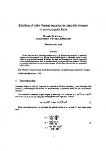
Incorporating uncertainty also in D, the covariance matrix of the residuals, is quite straightforward. Numerical example Let us consider a portfolio consisting of n = 7 stocks whose returns are determined affinely by 2 factors (for instance, the NASDAQ index, and the price of gold). Let us assume that the mean and covariance of these factors and the residuals are known. However, the sensitivity matrix is not certain. We assume that each element in this matrix can change inside a certain interval independently of the other elements of the sensitivity matrix (box uncertainty). The size of the intervals is defined as the uncertainty magnitude. We are looking for the investment policy which yields the minimal VaR at a confidence level of 95% (² = 0.05). The approximate robust counterpart to the portfolio problem, was formulated and solved,under these assumptions, using MATLAB and SeDuMi [24]. The values of the objective function (the minimal VaR of the portfolio) for different uncertainty magnitudes are presented in Figure 4.1. In addition, in order to compare between the nominal and the robust solutions, the VaR of the nominal portfolio was also calculated for sensitivity matrices corresponding to perturbation vectors at the corners of the box uncertainty set. The worst (maximal) VaR obtained in this procedure for each uncertainty magnitude is also presented in Figure 4.1. As expected, we can see that for both nominal and robust portfolios the VaR increases with the uncertainty magnitude. Comparing the two curves in Figure 4.1, it is evident that the approximate robust portfolio gives a better (smaller) VaR than the one obtained in the worst case scenario for the nominal portfolio for the same level of confidence. This means that the nominal portfolio can result in a larger loss than the maximal possible loss of the portfolio obtained from solving the approximate robust counterpart. This observation becomes more prominent when the uncertainty magnitude increases. The relative difference between the VaR of the approximate robust portfolio and the worst case Var of the nominal portfolio for different uncertainty magnitudes was also calculated. The results are presented in Figure 4.2. Figure 4.2 demonstrates that this relative difference can reach more than 40% for uncertainty magnitudes smaller than 1. In terms of loss of portfolios in the stock market, this is a large difference between performances of different portfolios.

31

16 14

worse VaR based on nominal portfolio VaR of robust portfolio

12

VaR

10 8 6 4 2 0 0

0.2

0.4 0.6 uncertainty magnitude

0.8

1

Figure 4.1: Minimal VaR vs. uncertainty magnitude for nominal and robust portfolios. Confidence level: 95%

4.3

An example : the stable grasp problem

The stable grasp problem emerges from robotics [23]. In this problem, we consider a rigid body held by N robot fingers. We denote the center of mass of the body as the origin. The robot fingers exert contact forces on the body at given points p1 , p2 , . . . , pN ∈ R3 . The inward pointing normal to the body surface at the ith contact point is given by the unit vector v i ∈ R3 , and the force applied at that point by f i ∈ R3 . Each contact force f i can be decomposed into two components: the component normal to the contact surface (v i )T f i v i and the tangential component (I − v i (v i )T )f i . We assume that the tangential component is due to static friction, so its magnitude cannot exceed the magnitude of the normal component times the friction coefficient µ > 0, meaning, k(I − v i (v i )T )f i k2 ≤ µ(v i )T f i ,

i = 1, . . . , N

(4.18)

These are called friction-cone constraints and are conic-quadratic constraints in the variables f i . In addition, let us denote by F ext , T ext the equivalents to the sum of external forces and torques, respectively, acting on the body at its center of mass. Static equilibrium of the body is characterized by the following six linear equations: PN

f i + F ext = 0 PN i=1i i ext i=1

p ×f +T

=0

(4.19)

The normal component of contact forces is bounded by the maximal force the robot 32

50

relative error [%]

40

30

20

10

0 0

0.2

0.4 0.6 uncertainty magnitude

0.8

1

Figure 4.2: Relative difference in the VaR of the approximate robust portfolio and the worst-case VaR of the nominal portfolio vs. uncertainty magnitude can exert or the maximal deformation stress the body can tolerate, i.e. (v i )T f i ≤ fmax ,

i = 1, . . . , N

(4.20)

The stable grasp problem is typically the problem of finding both the contact points, pi , and the contact forces to apply in them, f i , in order to keep the fingers in contact with the body. In this paper we will assume that the contact points are already known. Finding contact forces f i that satisfy the constraints (4.18), (4.19) and (4.20), is called finding a stable grasp. This is actually a feasibility problem. To make it an optimization problem we can add an objective function. For example: finding the ”gentlest stable grasp” is the problem of minimizing fmax when the variables f i , fmax are subject to (4.18), (4.19) and (4.20). Another example is finding the maximal external force that can be applied on the object that still maintains the stable grasp. This is the problem of maximizing F ext when the variables f i , F ext are subject to the constraints (4.18), (4.19) and (4.20). A major source of uncertainty in the stable grasp problem is the lack of accuracy in implementation. Another possible source of uncertainty is inaccuracy in describing the shape of the held body, meaning, the angles between the robot fingers and the body are not known accurately. This leads to uncertainty in the directions v i . Hence, the parameters both on the right hand and the left hand sides of the conic quadratic constraints (4.18) are uncertain, and moreover the uncertainty on both sides is dependent (both parameters depend on the uncertain v i ). Uncertainty can also be added in the friction coefficient, the external force and the external torque. Robustness is enabled via the adjustable friction 33

forces. As far as we know, no attempt to build a robust counterpart for the stable grasp problem was made. In what follows we will use Theorem 4.0.1 to do so. Let us assume a structured uncertainty for the contact directions v i : 





v1  .     v=  ..  =  vN





v01 L X  ..  +ρ ζ`  .   `=1 v0N



v`1 ..  .  

ζ ∈ V ⊂ RL

(4.21)

v`N

where the perturbations set V is an intersection of ellipsoids given by (2.3) and (2.4) and v` ∈ R3N , ` = 0, . . . , L are known vectors. If we neglect terms including ζj ζk , we end up with a structured uncertainty for the matrix (I − v i (v i )T ) as well: (I − v i (v i )T ) ≈ (I − v0i (v0i )T ) − ρ

L X

ζ` [v0i (v`i )T + v`i (v0i )T ] ζ ∈ V ⊂ RL

(4.22)

`=1

Now, according to Theorem (4.0.1), the approximated robust counterpart to the constraints (4.18) is the set of the following SDP constraints:     

P µ(v0i )T f i − β i − λik

ρwi [f i ]

k

− 12 (I − v0i (v0i )T )f i

∃(λik ≥ 0, k = 1, . . . , K, β i ≥ 0) :  ρ(wi )T [f i ] −[ 12 (I − v0i (v0i )T )f i ]T P i λk Qk

−ρ(U i )T [f i ]

−ρU i [f i ]

β iI

k

  º0 

i = 1, . . . , N, (4.23)

where : µ µ i T i [(v1 ) f , . . . , (v`i )T f i , . . . , (vLi )T f i ] = [(v1i , . . . , v`i , . . . , vLi )T f i ]T , 2 2 1 U i [f i ] = − [(v0i (v1i )T + v1i (v0i )T )f i , . . . , (v0i (v`i )T + v`i (v0i )T )f i , . . . , (v0i (vLi )T + vLi (v0i )T )f i ]. 2

(wi [f i ])T =

The robust counterpart of constraints (4.20) is found using Theorem 2.2.1 : ∃(µik ∈ RL , τki ∈ R, k = 1, . . . , K, i = 1, . . . , N ) : P i fmax − (v0i )T f i + ρ K k=1 τk ≥ 0 i = 1, . . . , N   −(v1i )T f i 1   PK .. 2 i  i = 1, . . . , N  . k=1 Qk µk =   i T i −(vL ) f i i kµk k2 ≤ τk k = 1, . . . , K, i = 1, . . . , N

(4.24)

Numerical example Let us consider a cylinder with mass M , height H = 0.12m and radius R = 0.03m which has to be held by N = 3 robot fingers. Let us further assume that the contact 34

points are on the same height h = 0m and are distributed equally on the periphery of the cylinder. Hence, the coordinates of the contact points are p1 = (R, 0, h)T , p2 = (−R cos 60◦ , R sin 60◦ , h)T , p3 = (−R cos 60◦ , −R sin 60◦ , h)T . The only external force applied on the cylinder is the gravitational force (0, 0, −gM ). No external torque exists. fmax = 10N . The friction coefficient, µ equals 0.3. This setting is schematically presented in Figure 4.3.

Figure 4.3: A cylinder held by 3 symmetrically positioned robot fingers. We are looking for the maximal mass of the cylinder (or equivalently, maximal external force) such that a stable grasp holds. For a cylinder held at its periphery, the normal to −pi the surface at a contact point is given by v0i = kp i k . Let us assume that any diversion from this direction is independent and isotropic for all fingers and for all directions (x,y or z). Note that since v i is a unit vector, only perturbation in the perpendicular direction to v i will affect its direction. Such a perturbation of size δ will cause a change in the norm of v i in the order of δ 2 and hence we assume that the norm change can be neglected for small perturbations. Based on all that, we consider the following perturbation set: V is a 2N -dimensional box-uncertainty set and v`i ` = 1, 2, are the orthonormal basis vectors of the two dimensional subspace perpendicular to v i , for i = 1, . . . , N . The approximate robust counterpart of the stable grasp problem (formulated in (4.19), (4.23) and (4.24)) was solved, under these assumptions, using MATLAB and SeDuMi [24]. The values of the objective function (the maximal mass of the cylinder that can be held maintaining stable grasp) for different magnitudes of perturbations are presented in Figure 4.4. In addition, in order to evaluate the quality of the approximation, the certain problem of the stable grasp was solved for perturbation vectors at the corners of the box uncertainty set for each perturbations magnitude (ρ). The worst (minimal) objective function value of these certain problems is also presented in Figure 4.4. It should be noted that unlike the results that were shown regarding the portfolio problem, here we do not compare two distinct solutions. The solution which yields the worst objective function value of this set of certain problems may be different for different perturbations magnitudes. The worst objective function value of the certain problems solved, merely serves as the upper bound to a robust objective function value (if we could find it). Comparing the two curves in Figure 4.4, it is seen that the approximate robust counterpart of the stable grasp problem is indeed a conservative approximation, since its 35

1

maximal cylinder mass [Kg]

0.9 0.8 0.7 0.6 0.5

worst of certain problems robust

0.4 0

0.02

0.04 0.06 perturbations magnitude

0.08

0.1

Figure 4.4: Maximal cylinder mass vs. perturbations magnitude (box uncertainty set) objective function value is lower (for a maximization problem) than the worst objective value of the certain problems. The relative error between the objective function value of the approximate robust counterpart and the worst objective function value of the certain problems for different perturbations magnitudes was calculated. The results are presented in Figure 4.5. Figure 4.5 demonstrates that the approximate robust counterpart approximates fairly well the worst-case scenario inside the uncertainty set. The relative error in the objective function is less than 9% for perturbations as large as 10%, which is a reasonable tolerance. The quality of the approximation deteriorates when the perturbations magnitude grows. The same analysis of the approximation quality for the stable grasp problem was carried out also for an ellipsoidal uncertainty set. Here, finding the worst case scenario is practically impossible. Hence, for each perturbations magnitude, 1000 perturbations vectors were taken randomly from the uncertainty set and the certain problem of the stable grasp was solved for each of them. The worst objective function of these certain problems for each perturbations magnitude is an inexact upper bound to the robust objective function value. This upper bound is compared with the objective function value yielded by the approximated robust counterpart in Figure 4.6. The relative error between the objective function value of the approximate robust counterpart and the worst objective function values of the certain problems for different magnitudes of perturbations is presented in Figure 4.7. Here again, we see that the approximate robust counterpart is indeed a conservative approximation which yields fairly good approximations: a relative error of less than 10% for perturbation magnitudes as large as 10%. 36

9 8

relative error [%]

7 6 5 4 3 2 1 0

0

0.02

0.04

0.06

0.08

0.1

perturbations magnitude

Figure 4.5: Relative error in maximal cylinder mass (between the approximate robust counterpart and the worst-case certain problem) vs. perturbations magnitude (box uncertainty set) We use this example also to compare between the approximate robust counterpart that was presented in section 3 (Theorem 4.0.1) and the one proposed by Bertsimas and Sim (Theorem 2.2.11). Let us assume a structured uncertainty for the contact directions v i (see (4.21)) where the perturbations set V is a unit ball and v` ∈ R3N , ` = 0, . . . , L are known vectors, calculated as was explained previously. If we neglect terms including ζj ζk , we end up with a structured uncertainty for the matrix (I −v i (v i )T ) as suggested in (4.22). Now, according to the result of Bertsimas and Sim (Theorem 2.2.11), a solution f i , M, i = 1, . . . , N • satisfies the constraints (4.18) if there exist βi ∈ R, ti ∈ RL , i = 1, . . . , N such that kti k2 i T i fmax − (v0 ) f −(v`i 0)T f i + t`i (v`i 0)T f i + t`i

≤ ≥ ≥ ≥

βi i = 1, . . . , N, ρβi i = 1, . . . , N, 0 i = 1, . . . , N, ` = 1, . . . , L 0 i = 1, . . . , N, ` = 1, . . . , L

(4.25)

• satisfies the constraints (4.20) if there exist αi ∈ R, ri ∈ RL , i = 1, . . . , N such that kri k2 i T i i i T µ(v0 ) f − k(I − v0 (v0 ) )f i k2 µ(v`i )T f i − k − [v0i (v`i )T + v`i (v0i )T ]f i k2 + ri` −µ(v`i )T f i − k[v0i (v`i )T + v`i (v0i )T ]f i k2 + ri`

37

≤ ≥ ≥ ≥

αi i = 1, . . . , N, (4.26) ραi i = 1, . . . , N, 0 i = 1, . . . , N, ` = 1, . . . , L 0 i = 1, . . . , N, ` = 1, . . . , L

maximal cylinder mass [kg]

1 worst of certain problems robust

0.9 0.8 0.7 0.6 0.5 0

0.02

0.04 0.06 perturbations magnitude

0.08

0.1

Figure 4.6: Maximal cylinder mass vs. perturbations magnitude (ellipsoidal uncertainty set) Combining (4.25),(4.26) and (4.19), results in another approximate robust counterpart of the stable grasp problem. Figure 4.8 shows the maximal cylinder mass (value of the objective function) calculated by solving the approximate robust counterpart suggested by Bertsimas and Sim and the one presented in Theorems 4.0.1 and 2.2.1 for different perturbations magnitudes. As can be expected, this mass decreases as the perturbations magnitude increases for both counterparts. However, it can be see that this decrease is steeper for Bertsimas and Sim’s robust counterpart. Figure 4.9 presents the relative difference in the objective function values of both approximations of the robust counterpart for different perturbations magnitude. This difference increases with the perturbations magnitude and reaches 17% for perturbations magnitude of 10%. This may suggest that the level of conservativeness of the approximated robust counterpart proposed by Bertsimas and Sim is larger than that of the approximted robust counterpart presented in Theorem 4.0.1.

38

10

relative error [%]

8

6

4

2

0 0

0.02

0.04 0.06 perturbations magnitude

0.08

0.1

Figure 4.7: Relative error in maximal cylinder mass (between the approximate robust counterpart and the worst-case certain problem) vs. perturbations magnitude (ellipsoidal uncertainty set)

1 Bertsimas and Sim Boni

maximal cylinder mass [kg]

0.9 0.8 0.7 0.6 0.5 0.4 0

0.02

0.04 0.06 perturbations magnitude

0.08

0.1

Figure 4.8: Maximal cylinder mass calculated based on the approximate robust counterparts of Boni and Bertsimas and Sim vs. perturbations magnitude (ellipsoidal uncertainty set) 39

18 16 relative difference [%]

14 12 10 8 6 4 2 0 0

2

4 6 8 perturbations magnitude [%]

10

Figure 4.9: Relative difference in maximal cylinder mass (between the approximate robust counterparts of Boni and Bertsimas and Sim) vs. perturbations magnitude (ellipsoidal uncertainty set)

40

Chapter 5 Affinely adjustable robust counterpart of conic constraints First, let us analyze the approach of adjustable variables for conic constraints. A conic constraint is of the form: Ax + b ∈ K, where K is some cone. If we denote by u, v the sub-vectors of the non-adjustable and the adjustable variables, respectively, we can write this constraint as: U u + Zv + b ∈ K.

(5.1)

Let us assume structured uncertainty and affine dependency of the adjustable variables in the perturbations vector, ζ, meaning, v = w+ρW ζ. Now, the constraint (5.1) becomes: U [ρζ]u + Z[ρζ](w + ρW ζ) + b[ρζ] ∈ K,

(5.2)

with the decision variables u, w, W . In the case of fixed recourse (matrix Z is certain) we look for u, w, W such that: D0 [u, w, W ] + ρ

L X

ζ` D` [u, w, W ] ∈ K

∀ζ ∈ V,

(5.3)

`=1

where D0 [u, w, W ] = U 0 u + Zw + B 0 , D` [u, w, W ] = U ` u + ZW` + b` . W` denotes the `-th column of W . The form (5.3) is very similar to (2.2), and hence Theorems 2.2.1–2.2.11 can be used to formulate the affinely adjustable robust counterpart for various perturbations sets.

41

In the case of variable recourse (at least one entry in matrix Z is uncertain) we look for u, w, W such that: D0 [u, w, W ] + ρ

L X

ζ` D` [u, w, W ] + ρ2

`=1

L X L X

ζ` ζk D`k [u, w, W ] ∈ K

∀ζ ∈ V,

(5.4)

`=1 k=1

where D0 [u, w, W ] = U 0 u + Z 0 w + B 0 , D` [u, w, W ] = U ` u + Z ` w + Z 0 W` + b` , D`k [u, w, W ] = Z ` Wk . W` denotes the `-th column of W . If we assume that the perturbations ζ are small enough, we can neglect the quadratic terms in ζ with respect to the affine terms in ζ. Thus, the small perturbations assumption results in a constraint very similar to (5.3) for which we can formulate a tractable counterpart (or an approximated counterpart). The assumption of small perturbations can be justified in many real-life applications. Otherwise, constraint (5.4) depends quadratically on the perturbations vector, so we cannot use Theorems 2.2.1–2.2.11 to find a tractable counterpart to it. A way to overcome this difficulty is to bind the quadratic term by γmin and γmax , meaning, min ζ∈V

max ζ∈V

L X L X `=1 k=1 L X L X

ζ` ζk D`k [u, w, W ] ≥ γmin , ζ` ζk D`k [u, w, W ] ≤ γmax .

`=1 k=1

Now, (5.4) is surely satisfied if ∀ζ ∈ V, δ ∈ [−1, 1]dimension of K : P min min + ρ L`=1 ζ` D` [u, w, W ] + ρ2 diag(δ) γmax −γ ∈ K. (5.5) D0 [u, w, W ] + ρ2 γmax +γ 2 2 Constraint (5.5) is very similar to (2.2), and hence Theorems 2.2.1–2.2.9 can be used to formulate an approximation to the affinely adjustable robust counterpart. Note that since the perturbations set in (5.5) is a direct product of the original perturbations set and an interval, the results of Bertsimas and Sim (Theorem 2.2.11) which assume a unit ball perturbations set cannot be applied here. As was mentioned before, affinely adjustable robust counterparts of linear constraints were already formulated. Now, let us use this outlined methodology for conic quadratic and semidefinite constraints.

5.1

Affinely adjustable robust counterpart of a conic quadratic constraint

Consider a conic quadratic constraint with structured uncertainty: kA[ρζ]x + b[ρζ]k2 ≤ cT [ρζ]x + d[ρζ]. 42

(5.6)

Let us denote by u, v the subvectors of non adjustable and adjustable variables respectively. So that (5.6) can be written as kU [ρζ]u + Z[ρζ]v + b[ρζ]k2 ≤ eT [ρζ]u + f T [ρζ]v + d[ρζ]

(5.7)

Let us assume that the adjustable variables depend affinely on the perturbations vector, v = w + ρW ζ. So that u, w, W are the new decision variables.

5.1.1

Fixed Recourse

First, let us consider the case of fixed recourse. Theorem 5.1.1 Consider the constraint (5.7) with structured uncertainty (2.1) of the parameters U, b, e and d. Let us further assume that the perturbations set V is an intersection of ellipsoids centered at the origin given by (2.3) and (2.4). Then, a solution u, v = w + ρW ζ satisfies (5.7) for all perturbations ζ ∈ V if there exist λk ≥ 0, k = 1, . . . , K and µ ≥ 0 such that 

K P

λk  α[u, w, W ] − µ − k=1    ρ β[u, w, W ]  2  − 12 α ˜ [u, w, W ]

 ρ T β [u, w, W ] 2 K P k=1

λ k Qk

˜ w, W ] − ρ2 β[u,

− 12 α ˜ T [u, w, W ]

   º 0, ρ ˜T − 2 β [u, w, W ]   

(5.8)

µI

where α ˜ = U 0 u + Zw + b0 , β˜` = U ` u + ZW` + b` ,

(5.9)

T

α = e0 u + f T w + d0 , T

β ` = e` u + f T W` + d` and W` denotes the `-th column of W . Proof: In the case of fixed recourse, matrix Z and the vector f are certain. Hence, constraint (5.7) can be written as ˜ w, W ]T ζk2 ≤ α[u, w, W ] + ρβ[u, w, W ]T ζ, k˜ α[u, w, W ] + ρβ[u,

(5.10)

˜ α and β are given by (5.9). Constraint of the form (5.10) has a tractable where α ˜ , β, approximated robust counterpart when the perturbations set is an intersection of ellipsoids (see Theorem 4.0.1). The approximation is written explicitly in (5.8).

43

5.1.2

Variable Recourse

In the case of variable recourse at least one entry in matrix Z or vector f is uncertain (indeed depends on ζ). Inserting the affine dependency of both the adjustable variables and the parameters on the perturbations into (5.7) we get k˜ α+ρ

L X `=1

ζ` β˜` + ρ2

L X L X

ζ` ζj G˜`j k2 ≤ α + ρ

`=1 j=1

L X

ζ` β ` + ρ2

L X L X

ζ` ζj G `j ,

(5.11)

`=1 j=1

`=1

where α ˜ [u, w, W ] = U 0 u + Z 0 w + b0 , β˜` [u, w, W ] = U ` u + Z ` w + Z 0 W` + b` , G˜`j [u, w, W ] = Z ` Wj , T

T

T

T

(5.12)

α[u, w, W ] = e0 u + f 0 w + d0 , T

β ` [u, w, W ] = e` u + f ` w + f 0 W` + d` , T

G `j [u, w, W ] = f ` Wj , and W` denotes the `-th column of W . First, let us consider the case of small perturbations, which is indeed the case in many real life applications. Theorem 5.1.2 Consider the constraint (5.7) with structured uncertainty (2.1) of the parameters U, Z, b, e, f and d. Let us assume that the perturbations set V is an intersection of ellipsoids centered at the origin given by (2.3) and (2.4). Let us further assume that the perturbations are small. Then, a solution u, v = w + ρW ζ satisfies (5.11) for all perturbations ζ ∈ V if there exists λk ≥ 0, k = 1, . . . , K and µ ≥ 0 such that 

K P

λk  α[u, w, W ] − µ − k=1    ρ β[u, w, W ]  2  − 12 α ˜ [u, w, W ]

 ρ T β [u, w, W ] 2 K P k=1

λ k Qk

˜ w, W ] − ρ2 β[u,

− 12 α ˜ T [u, w, W ]

   º 0. ρ ˜T − 2 β [u, w, W ]   

(5.13)

µI

˜ α, β are given by (5.12). where α ˜ , β, Proof: When the perturbations are small, the quadratic terms in ζ in (5.11) can be neglected, and this constraint becomes ˜ w, W ]T ζk2 ≤ α[u, w, W ] + ρβ[X]T ζ. k˜ α[u, w, W ] + ρβ[u,

(5.14)

Constraint of the form (5.14) has a tractable approximated robust counterpart when the perturbations set is an intersection of ellipsoids (see Theorem 4.0.1). The approximation is written explicitly in (5.13). 44

Now, we address the general case where the quadratic terms in the perturbations vector, ζ, cannot be neglected. Theorem 5.1.3 Consider the constraint (5.7) with structured uncertainty (2.1) of the parameters U, Z, b, e, f and d. Let us assume that the perturbations set V is an intersection of ellipsoids centered at the origin given by (2.3) and (2.4). Then, a solution u, v = w + ρW ζ satisfies (5.7) for all perturbations ζ ∈ V if there exist θ ≥ 0, hk ≥ 0, σi ≥ 0, λik , γi , µik , δi , νk , t, k = 1, . . . , K, i = 1, . . . , m such that  i  λk ≥ 0    K   P i

˜ i [u, w, W ] λ k Qk º Γ ,

(a)

k=1   K  P   λik ≤ γi  k=1  i  µk ≥ 0    K   P i

˜ i [u, w, W ] µ k Qk º − Γ , k=1

(b)

  K  P   µik ≤ −δi  k=1   νk ≥ 0    K   P

k=1   K  P   νk ≤ −t 

 2

 α+ρ t−θ−        

K P k=1

ρ β 2

k=1

hk −

m P i=1

k = 1, ..., K, 

ρ T β 2

σi

K P k=1

hk Qk

− ρ2 B

− 12 A where

i = 1, ..., m, k = 1, ..., K,

νk Qk º −G[u, w, W ] ,

(c)

(d)

i = 1, ..., m, k = 1, ..., K,



− 12 AT

    ρ T  º 0, −2B   ρ2 Diag{σ1 , ..., σm } − 2 C[δ, γ]   2

− ρ2 C T

θI (5.15) 

(G˜1,1 )i . . . (G˜1,L )i   .. .. ... ˜ i [u, w, W ] =  , Γ . .   L,1 L,L ˜ ˜ (G )i . . . (G )i





1 α ˜ 1 [u, w, W ] + ρ δ1 +γ 2   .. , A[u, w, W, δ, γ] =  .   δm +γm α ˜ m [u, w, W ] + ρ 2   β˜1T [u, w, W ]   .. , B[u, w, W ] =  .   T ˜ βm [u, w, W ]

(

)

γm − δm γ1 − δ 1 C[δ, γ] = diag , ..., , 2 2 45

(5.16)

˜ G, ˜ α, β, G are given by (5.12). and α ˜ , β, Proof: We denote y[ρζ, u, w, W ] = U [ρζ]u + Z[ρζ](w + ρW ζ) + b[ρζ]. The i-th coordinate in this vector can be represented as ˜ i [u, w, W ]ζ, yi [ρζ, u, w, W ] = α ˜ i [u, w, W ] + ρβ˜iT [u, w, W ]ζ + ρ2 ζ T Γ ˜ i [u, w, W ] is given by (5.16). where β˜i [u, w, W ] = [(β˜1 )i , . . . , (β˜L )i ] and Γ ˜ i [u, w, W ]ζ For every i = 1, . . . , m, we introduce an upper bound γi on the quantity max ζ T Γ ζ∈V

via the system of constraints λik ≥ 0, K P

k=1 K P k=1

i = 1, ..., m, k = 1, ..., K ˜ i [u, w, W ] λik Qk º Γ

(5.17)

λik ≤ γi

in variables λik , γi . Similarly, we introduce a lower bound δi on the quantity ˜ i [u, w, W ]ζ via the system of constraints min ζ T Γ ζ∈V

µik ≥ 0, K P

k=1 K P k=1

i = 1, ..., m, k = 1, ..., K ˜ i [u, w, W ] µik Qk º −Γ

(5.18)

µik ≤ −δi

in variables µik , δi . We also introduce an upper bound r on the quantity max ζ T G[u, w, W ]ζ via the system ζ∈V

of constraints

ηk ≥ 0 k = 1, ..., K K P k=1 K P k=1

ηk Qk º G[u, w, W ]

(5.19)

ηk ≤ r

in variables ηk , r. Similarly, we introduce a lower bound t on the quantity min ζ T G[u, w, W ]ζ ζ∈V

via the system of constraints νk ≥ 0, K P k=1 K P k=1

k = 1, ..., K

νk Qk º −G[u, w, W ] νk ≤ −t 46

(5.20)

in variables νk , t. The quantities λik , µik , γi , δi ,ηk , νk , r, t serve as additional decision variables. Now, for every ζ ∈ V, the value of the right hand side of the constraint (5.11) is inbetween the quantities α + ρβ T ζ + ρ2 t and α + ρβ T ζ + ρ2 r, and the value of yi [ρζ, u, w, W ] T is in-between the quantities α ˜ i + ρβ˜i ζ + ρ2 δi and α ˜ i + ρβ˜iT ζ + ρ2 γi . Next, we consider the following uncertain conic quadratic constraint in variables u, w, W , δi , γi , t, r: ´ ¯¯ ³ ¯¯ 1 1 α ˜ 1 + ρ2 δ1 +γ + ρβ˜1T ζ + ρ2 ²1 γ1 −δ ¯¯ 2 2 ¯¯ ¯¯ .. ¯¯ . ¯¯ ³ ´ ¯¯ δm +γm 2 T m ¯¯ α ˜m + ρ + ρβ˜m ζ + ρ2 ²m γm −δ 2 2

¯¯ ¯¯ ¯¯ µ ¶ ¯¯ t+r ¯¯ T 2 r−t ¯¯ ≤ α + ρ2 +ρβ ζ+ρ ² , (5.21) ¯¯ 2 2 ¯¯ ¯¯ 2

where the perturbations are (ζ, ²1 , . . . , ²m , ²) ∈ V × [−1, 1]m × [−1, 1]. It is clear that whenever a robust feasible solution (u, w, W, {γi , δi }m i=1 , t, r) of (5.21) i i can be extended, by properly chosen λk , µk , ηk , νk to solutions of (5.17), (5.18), (5.19), (5.20), the set (u, w, W ) is a solution to (5.11). Since the perturbation ² appears only on the left hand side of (5.21), the robust counterpart of this constraint is equivalent to the robust counterpart of the following constraint ´ ¯¯ ³ ¯¯ 1 1 + ρβ˜1T ζ + ρ2 ²1 γ1 −δ α ˜ 1 + ρ2 δ1 +γ ¯¯ 2 2 ¯¯ ¯¯ .. ¯¯ . ¯¯ ³ ´ ¯¯ T 2 δm +γm m ¯¯ + ρβ˜m α ˜m + ρ ζ + ρ2 ²m γm −δ 2 2

¯¯ ¯¯ ¯¯ ¯¯ ³ ´ ¯¯ ¯¯ ≤ α + ρ2 t + ρβ T ζ, ¯¯ ¯¯ ¯¯

(5.22)

2

where the perturbations are (ζ, ²1 , . . . , ²m ) ∈ V × [−1, 1]m . Note that constraint (5.22) is an uncertain conic quadratic constraint with the perturbation set which is an intersection of ellipsoids centered at the origin, and as such has a tight tractable approximation, according to Theorem 4.0.1. Replacing the robust counterpart of (5.22) with its tight tractable approximation (given explicitly in 5.15(d)), and adding the constraints (5.17), (5.18), (5.20) yields a tractable approximation of (5.7). Corollary 5.1.1 Consider the one sided conic quadratic constraint kAx + bk2 ≤ τ Let us denote by u, v the subvectors of non adjustable and adjustable variables, respectively. So that this constraint can be written as kU [ρζ]u + Z[ρζ]v + b[ρζ]k2 ≤ τ.

(5.23)

Let us assume structured uncertainty (2.1) of the parameters U, Z and b. Let us further assume that the perturbations set V is an intersection of ellipsoids centered at the origin given by (2.3) and (2.4). Then, a solution u, v = w + ρW ζ satisfies (5.23) for all perturbations ζ ∈ V if there exist θ ≥ 0, hk ≥ 0, σi ≥ 0, µik , δi , λik , γi , k = 1, . . . , K, i = 1, . . . , m such that 47

 i  λk ≥ 0, i = 1, ..., m, k = 1, ..., K    K   P ˜ i [u, w, W ] λik Qk º Γ k=1   K  P   λik ≤ γi  k=1  i   µk ≥ 0, i = 1, ..., m, k = 1, ..., K,   P   K i ˜

(a)

µk Qk º −Γi [u, w, W ]

(b) 

(c)

k=1   P   K i  µk ≤ −δi 

(5.24) 

k=1

K P

m P

hk − σi  τ −  i=1 k=1        A

A

K P k=1

hk Qk

ρB

Diag{σ1 , ..., σm } ρ2 C T

T

    ρB T   º 0,  2 ρC  

τI

˜ i [u, w, W ], A[u, w, W, δ, γ], B[u, w, W ], C[δ, γ] are given by (5.16). where Γ Proof: This tight approximation of the affinely adjustable robust counterpart of a one-sided conic quadratic constraint is found in a very similar way to a two-sided conic quadratic constraint. The only difference is that the right hand of the constraint is certain and there is no need to produce bounds for it. Hence, (5.23) can be approximated (similarly to (5.21)) by: ´ ¯¯ ³ ¯¯ 1 1 + ρβ˜1T ζ + ρ2 ²1 γ1 −δ α ˜ 1 + ρ2 δ1 +γ ¯¯ 2 2 ¯¯ ¯¯ .. ¯¯ ¯¯ ³ ´ . ¯¯ δm +γm 2 T m ¯¯ α ˜m + ρ + ρβ˜m ζ + ρ2 ²m γm −δ 2 2

¯¯ ¯¯ ¯¯ ¯¯ ¯¯ ¯¯ ≤ τ ¯¯ ¯¯ ¯¯

(5.25)

2

m

where the perturbations are (ζ, ²1 , ..., ²m ) ∈ V × [−1, 1] . The approximated robust counterpart to this constraint, according to Theorem 2.2.4, is given explicitly by (5.24(c)).

5.1.3

An example: subway route design

Let us consider the following problem of a subway route design. The route consists of subway stations and tunnels connecting them. The neightbourhoods which have to be served by the subway route (meaning, contain a subway station), and their boundaries are given. Let us assume that the tunnels between two consecutive stations are built in a straight line. We aim to minimize the total length of the tunnels, by choosing the stations locations which inside the neighbourhoods. The stations are built sequentially in a prescribed order. The problem can be formulated as follows: 48

n−1 X

min i 2

t∈Rn−1 ,x ∈R ,i=1,...,n

ti

i=1 i

subject to kxi+1 − x k2 ≤ ti i = 1, . . . , n − 1 xi ∈ Si i = 1, . . . , n,

(5.26)

where n is the number of stations to be located, xi ∈ R2 is their location (the decision variables) and Si is a set of possible locations (inside the neighbourhood) for the i-th station. In real life, the construction company building the subway stations might encounter all sorts of difficulties trying to implement the solution of (5.26). For example, discovering an archeological site or bumping into a water reservoir. Since the stations are built one after the other, once there is a deviation in the location of a certain station, the locations of the next (in the sense of building order) stations can be updated accordingly. This allows us to use the adjustable scheme. We assume implementation errors of the form: xi = x¯i (I + diag(ξ i )) i = 1, . . . , n, where xi , x¯i are the actual and planned locations of station i, respectively, and ξ i ∈ R2 is the actual relative error in the location of station i. We further assume affine dependency of the variables in the implementation errors: x¯i = wi + W i ξ

i = 1, . . . , n.

For simplicity, we consider the case of rectangular neighbourhoods, i.e. Si = {xi :

(LB)i ≤ xi ≤ (U B)i },

(5.27)

where (LB)i , (U B)i ∈ R2 are known boundaries of neighbourhood i. If we assume that the implementation errors, ξ, belong to an intersection of ellipsoids set given by (2.3) and (2.4), we can use corollary 5.1.1 to find the approximate affinely adjustable robust counterparts for the conic quadratic constraints in (5.26), and Theorem 2.4.3 to find the affinely adjustable robust counterparts for the linear constraints arising from (5.27). The result is the following semidefinite program in the decision variables t ∈ Rn−1 , wi ∈ R2 and the additional variables W i ∈ R2×2n , λik , γ i , µik , δ i ∈ R2 , hik ∈ R, σ i , τki , sik ∈ R2 , i = 1, . . . , n, k = 1, . . . , K : Pn−1

i=1 ti λik ≥ 0

min subject to K P

(λik )j Qk º Γi+1,j − Γi,j

k=1

P i λk ≤ γ i k

49

i = 1, ..., n, k = 1, ..., K, i = 1, ..., n, j = 1, 2 i = 1, ..., n

µik ≥ 0 K P

i = 1, ..., n, k = 1, ..., K,

(µik )j Qk º −(Γi+1,j − Γi,j )

k=1

i = 1, ..., n, j = 1, 2

P i µk ≤ −δ i

i = 1, ..., n

k



hik ≥ 0 σi ≥ 0 K P

 ti −  k=1       

  

hik

−

σ1i

−

i T

(A )

K P k=1

Ai

hik Qk diag{σ1i , σ2i } ρ2 (C i )T

ρB i

i

i

−(LB )j + (w )j −

τki ≥ 0 i k=1 (τk )j

PK

 

i

i

(U B )j − (w )j −

sik PK i k=1 (sk )j

− ρ2 ((β i )j )T

    ρ(B i )T   º 0 i = 1, ..., n − 1  2 i  ρC 

ti I

ρ (β i )j 2

ρ2 i,j G 2

ρ ((β i )j )T 2





σ2i

i = 1, ..., n, k = 1, ..., K i = 1, ..., n

+

PK

− ρ2 (β i )j −2G

i,j

+

 º0

i = 1, ..., n, k = 1, ..., K i = 1, ..., n, j = 1, 2,

i k=1 (τk )j Qk

≥0

ρ2



PK

  º0

i = 1, ..., n, k = 1, ..., K i = 1, ..., n, j = 1, 2

i k=1 (sk )j Qk

where βi = Di (wi ) + W i , Γi,j = Ri,j W i , Ai = (wi+1 − wi ) +

ρ2 i (γ + δ i ), 2

B i = (β i+1 − β i ), C i = diag(γ i − δ i ), T

Gi,j = Γi,j + Γi,j . Di (wi ) is a 2 × 2n matrix where all the entries are zero besides the [1 : 2, 2i + 1 : 2i + 2] block which contains the matrix diag(wi ). Ri,j is a 2n × 2 matrix where all the entries are zero besides the [2(i − 1) + j, j] entry which is equal to 1. The notation (z)j denotes the jth row in z. numerical example Consider a subway route comprised of n = 4 stations. The neighbourhoods map is given in Figure 5.1. The first station location is of course a non-adjustable variable, but the location of each other station is an adjustable variable which depends on the implementation errors in locating the former stations. For simplicity, we assume that the 50

stations are built according to their number (meaning, that station no. 1 is the first to be built, station no. 2 is the second to be built etc.). This imposes a certain structure on the matrices W i : W 1 = 0, and in W i , the rows corresponding to the perturbations ξ i+1 , . . . , ξ n contain only zeros. The perturbation set is assumed to be a box: −²i ≤ ξi ≤ ²i

i = 1, . . . , n,

where ξi , ²i ∈ R2 are the actual and the maximal relative errors possible for each station location, respectively. The nominal problem (no implementation errors), the approximate robust counterpart (based on Theorems 2.2.1 and 2.2.4) and the approximate affinely adjustable robust counterpart (5.28) of the problem were formulated and solved using MATLAB and SeDuMi [24]. In Figure 5.1 the nominal and the affinely adjustable robust solution are depicted for two cases. The first assumes no implementation errors and the second describes the situation for a specific vector of implementation errors chosen randomly. The figure demonstrates that the nominal solution, which is placing a station at the corner of each neighbourhood, results in shorter tunnels in the case of no implementation errors, but can become infeasible when implementation errors occur. The total length of the tunnels of the affinely adjustable robust solution is compared with the total length of the tunnels of the robust solution for different uncertainty magnitudes in Figures 5.2 and 5.3. As expected, the affinely adjustable robust solution yields a better (smaller) objective function. The improvement in the tunnels length increases with the uncertainty magnitude and can reach 11% for implementation errors as large as 20%. nominal station

Adjustable station

ξ10

ξ=0

Figure 5.1: Neighbourhoods (marked by grey squares) and subway stations locations (marked by rings) in the case of no implemetations error (ξ = 0), and for a randomly chosen implementation errors vector (ξ 6= 0).

51

minimal total tunnels length [Km]

5.5 5 4.5 4 3.5 robust total tunnels length adjustable total tunnels length

3 2.5 0

0.04

0.08 0.12 uncertainty magnitude

0.16

0.2

Figure 5.2: Minimal total tunnels length vs. uncertainty magnitude.

5.1.4

An example: retailer-supplier flexible commitments contracts

We consider the retailer-supplier flexible commitment problem [4]. This is a two-echelon T-period supply chain problem. A retailer faces uncertain demand by end costumers for a single product. The retailer orders from a single supplier and operates under a contract whereby he commits (at time zero) to a vector of order quantities over T periods, and then dynamically replaces these committed quantities with actual orders. The purpose of flexible commitments agreement between a retailer and a supplier is to assist both of them in facing the uncertainty that is associated with the external demand. The retailer provides the supplier with future commitments which are estimates of his future orders for a given number of future periods. The supplier uses the commitments as forecasts to determine his production capacity. In return, the supplier may offer him a discounted cost as long as his actual orders do not differ from the original commitments and certain penalties otherwise. At the beginning of the planning horizon, the retailer’s status is given through the parameter inv0 (initial inventory). The retailer, then, specifies a vector of commitments w = w1 , . . . , wT for the product. At the beginning of each period t, the retailer has an inventory invt and he orders a quantity xt from the supplier at a unit cost ct . The costumers then place their demands dt . Consequently, the retailer has to pay for storage, ht for every stored unit, and for shortage in the product, pt for each unit he fails to supply. Moreover, due to the stipulations in the contract, the retailer incurs two additional costs. The first is penalty due to deviations between committed and actual orders, which

52

relative difference in total length [%]

12 10 8 6 4 2 0 0

0.04

0.08 0.12 uncertainty magnitude

0.16

0.2

Figure 5.3: Relative difference in minimal tunnels length between usual and affinely adjustable robust solutions vs. uncertainty magnitude. here we assume is quadratic: rt2 (wt − xt )2 . The second penalty is on deviation between successive orders, which here we assume is given by: st |wt − wt−1 |. Note that the supplier wants to avoid deviations between successive commitments, but the size of this deviation is of less importance, while when looking at deviation of the actual orders from the commitments, the supplier is more affected by the size of the deviation. This is why we assume that the penalty on deviation between successive commitments depends linearly on the size of the deviation, while the penalty on deviation of the actual orders from the commitments depends quadratically on the size of this deviation. Also, there are upper and lower bounds on the order quantities in each period, (Qmin )t and (Qmax )t , respectively. The retailer’s challenge is to come up with an optimal ordering policy. If all the parameters are known, including the demand vector, then the problem can be formulated as: min

x,w,inv

PT

t=1 ct xt

+ ht max{0, invt } + pt max{0, −invt } + rt2 (xt − wt )2 +

s.t.

PT

t=2

invt = invt−1 + xt − dt t = 1, . . . , T (Qmin )t ≤ xt ≤ (Qmax )t t = 1, . . . , T wt ≥ 0 t = 1, . . . , T

This formulation can be rewritten as the following conic quadratic problem: min

x,w,inv,y,u,z

PT

t=1 ct xt

+ y t + ut + 53

PT

t=2 zt

st |wt − wt−1 | (5.28)

s.t.

invt = invt−1 + xt − dt (Qmin )t ≤ xt ≤ (Qmax )t yt ≥ ht invt yt ≥ −pt invt zt ≥ st (wt − wt−1 ) zt ≥ st (wt−1 − wt ) wt ≥ 0 ut ≥ 0   rt (xt − wt )   ut −1  ∈ L3  2

t = 1, . . . , T t = 1, . . . , T t = 1, . . . , T t = 1, . . . , T t = 2, . . . , T t = 2, . . . , T t = 1, . . . , T t = 1, . . . , T

(5.29)

t = 1, . . . , T

ut +1 2

In reality, the demands dt , uncertainty by:

t = 1, . . . , T are, of course, uncertain. We model this

dt = d0t + ρ

L X

ζ` d`t .

`=1

We further assume that the perturbations affecting those parameters belongs to an intersection of ellipsoids set given by (2.3) and (2.4). In order to formulate the usual robust counterpart of (5.29), we first incorporate the P Pt−1 equations defining the inventory level to get invt = inv1 + t−1 j=1 xj − j=1 dj , and then use Theorem 2.2.1. min x,w,y,u,z s.t.

PT

t=1 ct xt

+ yt + u t +

PT

t=2 zt

(5.30)

(Qmin )t ≤ xt ≤ (Qmax )t t = 1, . . . , T Pt−1 0 PK Pt−1 k yt − ht (inv1 + j=1 xj − j=1 dj ) − ρ k=1 τt ≥ 0 t = 1, . . . , T 

PK

1



ht

2 k  k=1 Qk µt = 

ht yt + pt (inv1 + PK

Pt−1 1  j=1 dj  ..  .  Pt−1 L j=1

t = 1, . . . , T

dj

kµkt k2 ≤ τtk k = 1, . . . , K PK Pt−1 0 k k=1 σt ≥ 0 t = 1, . . . , T j=1 dj ) − ρ j=1 xj −

Pt−1

k=1



1



−pt

Qk2 νtk =   −pt

Pt−1 1  j=1 dj  ..  .  Pt−1 L j=1

t = 1, . . . , T

t = 1, . . . , T

dj

kνtk k2 ≤ σtk zt ≥ st (wt − wt−1 ) zt ≥ st (wt−1 − wt ) wt ≥ 0

k = 1, . . . , K, t = 2, . . . , T t = 2, . . . , T t = 1, . . . , T 54

t = 1, . . . , T

ut ≥ 0 λkt ≥ 0   rt (xt − wt )  

t = 1, . . . , T t = 1, . . . , T

  ∈ L3

ut −1 2 ut +1 2

t = 1, . . . , T.

Since the commitments in the contract are made beforehand, it is obvious that the commitments and hence the variables zt are non adjustable variables. It is also clear that the order at the first period is also a non adjustable variable. However, the orders at periods t > 1 are adjustable variables which depend on the perturbations affecting the demands in the previous periods. Hence, the variables ut and yt are also non adjustable when t = 1, and adjustable variables depending on the perturbations of periods 1, ..., t − 1 when t > 1. Assuming affine dependency of the adjustable variables on the perturbations we can write: xt = mt + ρMt ζ yt = at + ρAt ζ ut = ft + ρFt ζ where Mt` = 0 t = 1, . . . , T, ` = t, . . . , T A`t = 0 t = 1, . . . , T, ` = t, . . . , T Ft` = 0 t = 1, . . . , T, ` = t, . . . , T Using Theorems 5.1.1 and 2.4.1, the approximated affinely adjustable robust counterpart of (5.29) is: min

E

m,M,w,a,A,f,F,z,E

subject to E −

PT

t=1 (ct mt

PK

k=1

(5.31)

+ at + ft ) −

PT

t=2 zt

−ρ

PK

k=1

ϕk ≥ 0

P

1

Qk2 χk = − Tt=1 (ct Mt + At + Ft ) kχk k2 ≤ ϕk P k Qmax − mt − ρ K k=1 τt ≥ 0 PK

1

Qk2 µkt = −Mt kµkt k2 ≤ τtk P k mt − Qmin − ρ K k=1 σt ≥ 0 k=1

PK

1

Qk2 νtk = Mt kνtk k2 ≤ σtk PK P Pt−1 k 0 at − ht (inv1 + j=1 mj − t−1 k=1 φt ≥ 0 j=1 dj ) − ρ k=1

55

k = 1, . . . , K t = 1, . . . , T t = 1, . . . , T k = 1, . . . , K t = 1, . . . , T t = 1, . . . , T k = 1, . . . , K, t = 1, . . . , T

t = 1, . . . , T

t = 1, . . . , T





d1j 1   Pt−1 Pt−1 PK k 2  ..  k=1 Qk Φt = At − ht ( j=1 Mj − j=1  . ) dLj kΦkt k2 ≤ φkt P Pt−1 0 PK k at + pt (inv1 + t−1 j=1 mj − j=1 dj ) − ρ k=1 ψt ≥ 0 



d1j 1  Pt−1 Pt−1  .  PK k 2 .  j=1  . ) k=1 Qk Ψt = At + pt ( j=1 Mj − dLj kΨkt k2 ≤ ψtk zt ≥ st (wt − wt−1 ) zt ≥ st (wt−1 − wt ) wt ≥ 0 P k ft − ρ K k=1 πt ≥ 0 PK

     

ft +1 2

− θt −

K P k=1

ρ (Ft )T 4 − 21 At

λkt

1

ρ (Ft )T 4 K P k=1

k = 1, . . . , K, t = 1, . . . , T

t = 1, . . . , T k = 1, . . . , K, k = 1, . . . , K,



t = 1, . . . , T

t = 1, . . . , T k = 1, . . . , K, t = 2, . . . , T t = 2, . . . , T t = 1, . . . , T t = 1, . . . , T

2 k k=1 Qk ηt = Ft kηtk k2 ≤ πtk θt , (λkt ) ≥ 0



t = 1, . . . , T

t = 1, . . . , T

t = 1, . . . , T t = 1, . . . , T

− 12 ATt

λkt Qk

   ρ T  º 0 − 2 Bt  

− ρ2 Bt

t = 1, . . . , T

θt I2

where "

At [m, M, w, f, F ] = "

Bt [m, M, w, f, F ] =

rt (mt − wt ) ft −1 2

rt Mt Ft 2

#

,

#

,

numerical example Now, let us assume box uncertainty of the demands: dt ∈ [d0t (1 − ρ), d0t (1 + ρ)] t = 1, . . . , T.

(5.32)

This means that the perturbations affecting the demands at each period belong to independent intervals. We set the planning horizon to be T = 6 months, and the other parameters to be: d0 = (110, 120, 130, 140, 150)T , rt = 2 t = 1, . . . , T, ct = 15 t = 1, . . . , T, 56

ht pt st inv1 (Qmin )t (Qmax )t

= = = = = =

2 t = 1, . . . , T, 5 t = 1, . . . , T, 6 t = 1, . . . , T − 1, 100, 0 t = 1, . . . , T, 200 t = 1, . . . , T.

The nominal problem (5.29), the approximate robust counterpart (5.30) and the approximate affinely adjustable robust counterpart (5.31) of the problem were formulated and solved using MATLAB and SeDuMi [24]. In order to determine the price of robustness of the usual robust counterpart and compare it to the price of robustness of the affinely adjustable robust counterpart the following procedure was carried out. First, 1000 demand vectors were randomly chosen from the appropriate intervals. For each one of the demand vectors the certain problem (5.29) was solved. Note that this gives us the best solution one can achieve, since this is the ideal case where the demands are known in advance. Then, the robust counterpart was solved, yielding commitments and orders for each period. Note that the robust solution does not depend on the specific demands vector. The affinely adjustable robust counterpart was also solved yielding the commitments and an optimal orders policy. Inserting the demands vector into this policy gives the actual orders for this specific realization. The retailer’s costs of the ideal solution, the robust solution and the affinely adjustable robust solution (commitments and orders) were calculated using E=

T X

ct xt + ht max{0, invt } + pt max{0, −invt } + rt2 (xt − wt )2 +

t=1

T X

st |wt − wt−1 |. (5.33)

t=2

Finally, the mean and standard deviation of the cost using the ideal, robust and affinely adjustable robust solutions were calculated. This was done for several uncertainty magnitudes (which are equivalent to the intervals sizes). The results are presented in tables 5.1 and 5.2. The percentage of the difference between the expenses in the ideal case and the robust or affinely adjustable robust solutions is called the price of robustness. Uncertainty ρ 10 % 20 % 30 % 40 %

RC ideal mean std mean 8344 197 8255 8440 356 8242 8619 513 8238 8819 628 8271

case std 238 469 747 989

price of robustness 1.1% 2.4% 4.6% 6.6%

Table 5.1: The mean and standard deviation of the retailer’s cost in flexible commitments contract for ideal and robust solutions. The demands vary in an interval uncertainty of the size 2ρ. First, it should be noted that even though the robust solution itself is the same for all demands vectors, the cost E calculated based on this solution using (5.33) do vary since 57

Uncertainty ρ 10 % 20 % 30 % 40 %

AARC mean std 8273 244 8284 484 8331 799 8438 1079

ideal mean 8255 8242 8238 8271

case std 238 469 747 989

price of robustness 0.2% 0.5% 1.1% 2.0%

Table 5.2: The mean and standard deviation of the retailer’s expenses in flexible commitments contract for ideal and affinely adjustable robust solutions. The demands vary in an interval uncertainty of the size 2ρ. the cost depends on the number of stored units or the shortage size which vary with the demands. The results presented in tables 5.1 and 5.2 reveal that the price of robustness when using the affinely adjustable robust counterpart is surprisingly low, and grows very slowly with the level of uncertainty. It also outperforms the usual robust counterpart solution in terms of the price of robustness by a factor of 3 to 4. In addition, the price of robustness increases with the uncertainty magnitude for both the robust and the affinely adjustable robust solutions.

5.2

Affinely adjustable robust counterpart of a semidefinite constraint

Let us consider a semidefinite constraint with structured uncertainty: A0 [ρζ] +

n X

xi Ai [ρζ] º 0.

i=1

Let us assume without loss of generality that the first s variables are the non adjustable variables and the last n − s variables are the adjustable variables. If we denote by u and v the non-adjustable and the adjustable variables, respectively, then the constraint can be written as: s n A0 [ρζ] +

X

ui Ai [ρζ] +

i=1

X

vj Aj [ρζ] º 0

(5.34)

j=s+1

Let us further assume affine dependency of the adjustable variables on the perturbations, namely v = w + ρW ζ where w ∈ Rn−s , W ∈ R(n−s)×L are the new decision variables along with u.

5.2.1

Fixed Recourse

First, let us consider the case of fixed recourse.

58

Theorem 5.2.1 Consider the constraint (5.34) with structured uncertainty (2.1) of the parameters Ai , i = 1, . . . , s. Let us further assume that the perturbations set V is an intersection of ellipsoids centered at the origin given by (2.3) and (2.4). Then, a solution u, v = w + ρW ζ satisfies (5.34) for all perturbations ζ ∈ V if x satisfies: 

D0

 √ PL  ρ K `=1 E`,1 D`   ..  .  √ PL

ρ K

`=1

√ P √ P ρ K L`=1 E`,1 D` . . . ρ K L`=1 E`,L D` D0 0 0 .. . 0 0

E`,L D`

0

0

     º 0,  

D0 (5.35)

where E = (

K X

1

Qk )− 2

k=1

D0 [u, w, W ] = A00 + D` [u, w, W ] = A`0 +

s X i=1 s X

ui A0i + ui A`i +

i=1

n X j=s+1 n X

wj Aj

(5.36)

Wj` Aj

j=s+1

Wj` is the entry in line j and column ` of the matrix W . Proof: In the case of fixed recourse (matrices Aj , j = s + 1, . . . , n are certain), (5.34) can be written as: D0 [u, w, W ] + ρ

L X

ζ` D` [u, w, W ] º 0,

(5.37)

`=1

where D0 , D` , ` = 1, . . . , L are given by (5.36). Constraint of the form (5.37) has a tractable approximated robust counterpart when the perturbations set is an intersection of ellipsoids (see Theorem 2.2.9). The approximation is written explicitly in (5.35).

5.2.2

Variable Recourse

In the case of variable recourse at least one entry in matrices Aj , j = s + 1, . . . , n is uncertain (indeed depends on ζ). In this case the constraint (5.34) can be written as: D0 [u, w, W ] + ρ

L X

ζ` D` [u, w, W ] + ρ

2

`=1

L X L X `=1 k=1

59

ζ` ζk D`k [u, w, W ] º 0,

(5.38)

where D0 [u, w, W ] = A00 + D` [u, w, W ] = A`0 +

s X i=1 s X

ui A0i + ui A`i +

i=1

D`k [u, w, W ] =

n X

n X

wj A0j

j=s+1 n X

[(Wj )` A0j + wj A`j ]

(5.39)

j=s+1

[(Wj )k A`j ].

j=s+1

For small perturbations we have: Theorem 5.2.2 Consider the constraint (5.34) with structured uncertainty (2.1) of the parameters A0 , Ai , i = 1, . . . , s, . . . , n. Let us assume that the perturbations set V is an intersection of ellipsoids centered at the origin given by (2.3) and (2.4). Let us further assume that the perturbations are small. Then, a solution u, v = w + ρW ζ satisfies (5.34) for all perturbations ζ ∈ V if x satisfies   √ PL √ PL K E D . . . ρ K E D D ρ `,1 ` `,L ` 0 `=1 `=1  √ PL   ρ K  E D D 0 0 `,1 ` 0 `=1     º 0, (5.40) .. ..   . . 0 0  √  P ρ K L`=1 E`,L D` 0 0 D0 where E = (

PK

k=1

1

Qk )− 2 and D0 [u, w, W ], D` [u, w, W ] are given by (5.39).

Proof: When the perturbations are small, the quadratic terms in ζ in (5.38) can be neglected, and this constraint becomes D0 [u, w, W ] + ρ

L X

ζ` D` [u, w, W ] º 0,

(5.41)

`=1

where D0 [u, w, W ], D` [u, w, W ] are given by (5.39).. Constraint of the form (5.41) has a tractable approximated robust counterpart when the perturbations set is an intersection of ellipsoids (see Theorem 2.2.9). The approximation is written explicitly in (5.40).

Now, let us consider the case where the quadratic terms in the perturbations vector, ζ, cannot be neglected. Theorem 5.2.3 Consider the constraint (5.34) with structured uncertainty (2.1) of the parameters A0 , Ai , i = 1, . . . , s, . . . , n. Let us assume that the perturbations set V is an intersection of ellipsoids centered at the origin given by (2.3) and (2.4).

60

Then, a solution u, v = w + ρW ζ satisfies (5.34) for all perturbations ζ ∈ V if there f,g exist matrices gamma, δ ∈ Rm×m , λf,g k , µk , f, g = 1, ..., m, k = 1, ..., K such that:  f,g  λk ≥ 0,    K   P f,g

(a)

            

(b) 

(c)

k=1

λk Qk º Γf,g [u, w, W ]

λf,g k ≤ γf,g

µf,g k ≥ 0, K P

f, g = 1, ..., m, k = 1, ..., K

λf,g k Qk º −Γf,g [u, w, W ]

k=1   K  P    λf,g k ≤ −δf,g

D +  0                   

k=1 K P

f, g = 1, ..., m, k = 1, ..., K

ρ2 (γ 2

D1 .. . DL R1,1 R1,2 .. .



k=1

+ δ) D1 . . . DL R1,1 R1,2 . . . .. . .. . .. . .. . ... ...

Rm,m

Rm,m

D0 +

ρ2 (γ 2

           º 0,         

(5.42)

+ δ)

where 

Γf,g

Di



(D11 )f,g . . . (D1L )f,g   .. .. ... , =  . .   (DL1 )f,g . . . (DLL )f,g L √ X E`,i D` , = ρ K + m2

(5.43)

`=1

E = (

K X

1

Qk )− 2 ,

k=1

D0 [u, w, W ], D` [u, w, W ] are given by (5.39) and Rf,g ∈ Rm×m is a matrix of all zeroes 2√ but the entry in line f and column g which is equal to ρ2 K + m2 (γf,g − δf,g ). Proof: We first try to bind the quadratic terms in the perturbations vector which appear in constraint (5.38). P P Let us denote by Θ the matrix L`=1 Lk=1 ζ` ζk D`k [u, w, W ]. Every entry in Θ can be presented as Θf,g = ζ T Γf,g ζ where Γf,g is given by (5.43).

61

For every f, g = 1, . . . , m, we introduce an upper bound γf,g on the quantity max ζ T Γf,g ζ via the system of constraints: ζ∈V

λf,g k ≥ 0, K P

k=1 K P k=1

f, g = 1, ..., m, k = 1, ..., K

λf,g k Qk º Γf,g [u, w, W ]

(5.44)

λf,g k ≤ γf,g

in variables λf,g Similarly, we introduce a lower bound δf,g on the quantity k , γf,g . T min ζ Γf,g ζ via the system of constraints: ζ∈V

µf,g k ≥ 0, K P

k=1 K P k=1

f, g = 1, ..., m, k = 1, ..., K

λf,g k Qk º −Γf,g [u, w, W ]

(5.45)

λf,g k ≤ −δf,g

in variables µf,g k , δf,g . The matrices γ, δ are additional decision variables. Hence, the constraint (5.38) can be written as the following uncertain semidefinite constraint in variables u, w, W , γ and δ: 



²1,1 (γ1,1 − δ1,1 ) . . . ²1,m (γ1,m − δ1,m ) L X  ρ2 ρ2  .. .. ..   º 0 (5.46) D0 + (γ +δ)+ρ ζ ` D` +  . . .  2 2 `=1 ²m,1 (γm,1 − δm,1 ) . . . ²m,m (γm,m − δm,m ) where the perturbations are (ζ, ²) ∈ V × [−1, 1]m×m . Note that constraint (5.46) is an uncertain semidefinite constraint with the perturbation set which is an intersection of ellipsoids centered at the origin, and as such has a tight tractable approximation according to Theorem 2.2.9. Replacing the robust counterpart of (5.46) with its tight tractable approximation (written explicitly in (5.42(c))), and adding the constraints (5.44) and (5.45) yields a tractable approximation of (5.34).

62

Chapter 6 Mixed Uncertainty So far, we assumed that the uncertainty affecting a certain constraint is either bounded or probabilistic. However, in reality, it may well happen that the values of some parameters of the constraint are random variables with known probability distribution, while the other parameters are uncertain and known only to belong to a bounded set. In other words, the uncertainty affecting the constraint is mixed. Some of the parameters are affected by probabilistic uncertainty , while the other parameters suffer from set inclusion uncertainty. In what follows we define robust feasible solutions to such constraints and develop a scheme to formulate their robust counterparts. Let us consider a conic constraint with structured mixed uncertainty. A[ρζ, ρξ]x + b[ρζ, ρξ] ∈ K where K is a convex, pointed cone, 0

0

[A[ρζ, ρξ], b[ρζ, ρξ]] = [A , b ] + ρ

L X

`

`

ζ` [A , b ] + ρ

`=1

Q X

ξq [E q , f q ]

q=1

ρ > 0 is the perturbations magnitude and the perturbations themselves can be divided into two types: • (i) ζ runs through an intersection of ellipsoids centered at the origin: ζ ∈ V = {ζ : ζ T Qk ζ ≤ 1, k = 1, ..., K}

[Q` º 0,

P `

Q` Â 0]

• (ii) ξ1 , ..., ξQ are random variables with zero means and “light tails”, o n independent √ 2 specifically, E exp{ξq /4} ≤ 2. We are looking for a solution x such that: ∀ζ ∈ V : Prob {A[ρζ, ρξ]x + b[ρζ, ρξ] ∈ K} ≥ 1 − ², for a given unreliability level ². 63

(6.1)

To this end, we bound the probabilistic perturbations inside a ball kξk2 ≤ Γ such that Prob {A[ρζ, ρξ]x + b[ρζ, ρξ] ∈ K} ≥ 1 − ². Γ is called the safety factor and its dependency on the unreliability level ² can be determined using Theorem 2.3.1. Now, ensuring ∀ζ ∈ V, kξk2 ≤ Γ : A[ρζ, ρξ]x + b[ρζ, ρξ] ∈ K

(6.2)

ensures that x satisfies (6.1) Constraint (6.2) is in fact a convex conic constraint with structured uncertainty and a perturbations set which can be presented as an intersection of (K + 1) ellipsoids. Hence we can use Theorems 2.2.1–2.2.11 to formulate the robust counterpart of (6.2). Thus, we obtain a sufficient condition for x being feasible to (6.1). In what follows we formulate specifically the counterparts for (6.1) for the cases of linear, conic quadratic and semidefinite constraints.

6.1

Mixed uncertainty in a linear constraint

An uncertain linear constraint with structured mixed uncertainty is of the form: a[ρζ, ρξ]T x + b[ρζ, ρξ] ≥ 0 with [b, ai ] = [b

0

, a0i ]

+ρ

L X

`

ζ` [b

, a`i ]

+ρ

Q X

(6.3) ξq [dq , cqi ].

(6.4)

q=1

`=1

ζ, ξ being set bounded and random perturbations, respectively. We are looking for a solution x such that ∀ζ ∈ Z : Prob {A[ρζ, ρξ]x + b[ρζ, ρξ] ≥ 0} ≥ 1 − ².

(6.5)

Theorem 6.1.1 Consider the linear constraint (6.3) with structured mixed uncertainty (6.4). ζ, ξ satisfy (i) and (ii). Then, a solution x satisfies (6.5) if there exist τk ∈ R, µk ∈ RL , k = 1, . . . , K such that: ° P ° d1 + ni=1 c1i xi ° ° .. (a0 )T x + b0 − ρΓ °° .  ° P ° dQ + n cQ xi i=1 i 

° ° ° ° ° + ρ PK τk ≥ 0 k=1 ° ° ° 2 

(a1 )T x + b1   PK ..   . k=1 Qk µk =   (aL )T x + bL kµk k2 ≤ τk k = 1, . . . , K 1 2

q

where Γ = O(1) ln( 1² ). 64

Proof: First, let us rewrite (6.3) as: r[x] + ρR[x]T ζ + ρ

Q X

ξq [(cq )T x + dq ] ≥ 0,

q=1

where r[x] = (a0 )T x + b0 , R[x] = [(a1 )T x + b1 , . . . , (aL )T x + bL ]T . Based on Theorem 2.3.2, for every ζ ∈ V  

Prob r[x] + ρR[x]T ζ + ρ if

Q X q=1

 

ξq [(cq )T x + dq ] ≥ 0 ≥ 1 − ²,

° P ° d1 + ni=1 c1i xi ° ° .. r[x] + ρR[x]T ζ − ρΓ °° .  ° Pn Q Q ° d + i=1 ci xi q

° ° ° ° ° ≥ 0 ° ° °

(6.6)

2

where the safety factor Γ = O(1) ln( 1² ). Now, all we have to ensure is that x satisfies (6.6) for all ζ ∈ V. Using Theorem 2.2.1, this happens if and only if there exist τk ∈ R, µk ∈ RL , k = 1, . . . , K such that (x, τ, µ) satisfies: ° P ° d1 + ni=1 c1i xi ° ° .. r[x] − ρΓ °° .  ° Pn Q Q ° d + i=1 ci xi PK

° ° ° ° P ° + ρ K τk ≥ 0 k=1 ° ° ° 2

1 2

Qk µk = R[x] kµk k2 ≤ τk k = 1, . . . , K k=1

Similar theorem can be proved in a very similar way for the case where the bounded perturbations vector, ζ, belongs to a semidefinite representable set, using Theorems 2.3.2 and 2.2.2. The resulting approximate robust counterpart is a semidefinite program.

6.2

Mixed uncertainty in a conic quadratic constraint

A conic quadratic constraint with mixed structured uncertainty is of the form: kA[ρζ, ρξ]x + b[ρζ, ρξ]k2 ≤ c[ρζ, ρξ]T x + d[ρζ, ρξ] 65

with [A, b, c, d] = [A0 , b0 , c0 , d0 ] + ρ

L X

ζ` [A` , b` , c` , d` ] + ρ

Q X

ξq [E q , f q , g q , hq ],

(6.7)

q=1

`=1

where ζ belong to the bounded uncertainty set V, and ξ are random perturbations.

6.2.1

One-sided uncertainty

First, let us consider an uncertain one-sided conic quadratic constraint kA[ρζ, ρξ]x + b[ρζ, ρξ]k2 ≤ τ.

(6.8)

Note that in this type of constraint only the left hand side is uncertain. We are interested in finding a solution x, τ such that: ∀ζ ∈ V : Prob {kA[ρζ, ρξ]x + b[ρζ, ρξ]k2 > τ } ≤ ².

(6.9)

Theorem 6.2.1 Consider the constraint (6.8) with structured uncertainty (6.7). ζ, ξ satisfy (i) and (ii). Then, a solution x satisfies (6.9) if there exist µ ≥ 0, λk ≥ 0, σ, νk , χ, k = 1, . . . , K such that: 



K P

λk − µ  τ −  k=1   (a)     

T

u [x]

K P k=1

u[x] 

(b)

(d)

µI ρΓW [x]

ρV [x] K P

νk  σ−  k=1     u[x] ¯¯  ¯¯

(c)

λk Qk

    ρV T [x]  º0  ρΓW T [x]   

τI

uT [x] 

K P k=1

νk Qk

ρV [x] W11 [x] W12 [x] .. .

   º 0, ρV T [x]  

(6.10)

σI

¯¯ ¯¯ ¯¯ ¯¯ ¯¯ ¯¯ ¯¯ ¯¯ ¯¯ ≤ χ, ρΓ ¯¯¯¯  ¯¯ ¯¯ ¯¯ ¯¯ ¯¯ ¯¯ WmQ [x] ¯¯ 2 °" #° ° σ ° ° ° ° ° ≤τ ° χ ° 2

where u[x] = A0 x + b0 , V [x] = (A1 x + b1 , . . . , AL x + bL ), W [x] = (E 1 x + f 1 , . . . , E Q x + f Q )

(6.11)

q

Wij is the element on row i and column j of matrix W and Γ = O(1) ln(1/²) 66

Proof: Note that the vector A[ρζ, ρξ]x + b[ρζ, ρξ] can be represented as u + ρV ζ + ρW ξ, where the vector u[x] and the matrices V [x], W [x] are given by (6.11). Thus, constraint (6.8) is equivalent to the relations τ ≥ 0,

y T [ρζ]y[ρζ] + 2ρξ T W T y[ρζ] + ρ2 ξ T W T W ξ ≤ τ 2 ,

where y[ρζ] = u + ρV ζ. Now consider the following conditions: (a) ∀(ζ ∈ V, ξ : kξk2 ≤ 1) : y T [ρζ]y[ρζ] + 2Γρξ T W T y[ρζ] + ρ2 Γ2 ξ T W T W ξ ≤ τ 2 , (b) ∀(ζ ∈ V) : y T [ρζ]y[ρζ] + ρ2 Γ2 Tr(W T W ) ≤ τ 2 , where Γ is called a safety parameter. Using non-negativity of a third term in (6.12(a)) and a particular ξ = relations in (6.12) yield:

(6.12)

WTy , kW T yk

the

(a) ∀(ζ ∈ V) : y T [ρζ]y[ρζ] + 2ΓρkW T y[ρζ]k2 ≤ τ 2 , (b) ∀(ζ ∈ V) : y T [ρζ]y[ρζ] + ρ2 Γ2 Tr(W T W ) ≤ τ 2 . √

Taking κ = 5−1 (so that κ = 1 − κ2 ), multiplying (a) by κ and (b) by κ2 = 1 − κ and 2 adding the results, we arrive at ∀(ζ ∈ V) : y T [ρζ]y[ρζ] + 2ΓκρkW T y[ρζ]k2 + Γ2 ρ2 κ2 Tr(W T W ) ≤ τ 2 .

(6.13)

Observe that when ξ1 , ..., ξQ are independent zero mean random variables with light tails, we have by Theorem 2.3.1: n

o

Prob ξ T W T y[ρζ] > ΓκkW T y[ρζ]k2 ≤ O(1) exp{−O(1)Γ2 }, n

o

Prob ξ T W T W ξ > Γ2 κ2 Tr(W T W ) ≤ O(1) exp{−O(1)Γ2 }, whence (6.12) ⇒ (6.13) ⇒½

¾

∀(ζ ∈ V) : Prob y T [ρζ]y[ρζ] + 2ρξ T W T y[ρζ] + ρ2 ξ T W T W ξ ≥ τ 2 ≤ O(1) exp{−O(1)Γ2 }, |

{z

}

ku+ρV ζ+ρW ξk22

q

(6.14)

so that relations (6.12) with Γ = O(1) ln(1/²) ensure (6.9). Now, observe that (6.12(a)) is equivalent to the fact that (x, τ ) is robust feasible for the conic quadratic constraint : kA[ρζ, ρΓξ]x + b[ρζ, ρΓξ]k2 ≤ τ, 67

with a bounded uncertainty set being V + = {(ζ, ξ) : ζ T Qk ζ ≤ 1, k = 1, ..., K, ξ T ξ ≤ 1}, that is, being the intersection of ellipsoids centered at the origin. Hence, by Theorem 2.2.4, (6.12(a)) has a tractable approximated robust counterpart which is written explicitly in (6.10(a)). Similarly, (6.12(b)) is equivalent to the fact that (x, τ ) is robust feasible for the uncertain conic quadratic constraint ¯¯ ¯¯ u[x] + ρV [x]ζ ¯¯ ¯¯ ¯¯ ρΓW11 [x] ¯¯ ¯¯ ρΓW12 [x] ¯¯ ¯¯ .. ¯¯ . ¯¯ ¯¯ ¯¯ ρΓWM Q [x]

¯¯ ¯¯ ¯¯ ¯¯ ¯¯ ¯¯ ¯¯ ¯¯ ≤ τ, ¯¯ ¯¯ ¯¯ ¯¯ ¯¯ 2

This constraint can be replaced by the following set of conic quadratic constraints: ku[x] + ρV [x]ζk2 ≤ σ,

¯¯ ¯¯ ¯¯ ¯¯ ¯¯ ¯¯ ¯¯ ¯¯ ¯¯ W11 [x] ¯¯ ¯¯ ¯¯ ¯¯ ρΓ ¯¯¯¯  W12 [x] ¯¯ ≤ χ, ¯¯ ¯¯ .. ¯¯ ¯¯ . ¯¯ ¯¯ ¯¯ ¯¯ ¯¯ WmQ [x] ¯¯ ¯¯" #¯2¯ ¯¯ σ ¯¯ ¯¯ ¯¯ ¯¯ ¯¯ ≤ τ, ¯¯ χ ¯¯

(6.15)

(6.16)

(6.17)

2

in variables x, τ, σ and χ. The remaining uncertainty lies only in (6.15) with the perturbation set being V, which is an intersection of ellipsoids. Therefore, replacing (6.15) with its approximated robust counterpart (written explicitly in (6.10(b)) according to Theorem 2.2.4) and adding (6.16) and (6.17), constructs a computationally tractable approximation of (6.12(b)). Thus, (6.12), which is a sufficient condition for the validity of (6.9), admits a computationally tractable approximation for (6.9).

6.2.2

Two-sided uncertainty

Now let us consider the conic quadratic constraint: kA[ρζ, ρξ]x + b[ρζ, ρξ]k2 ≤ c[ρζ, ρξ]T x + d[ρζ, ρξ]

(6.18)

where ζ belong to a bounded uncertainty set V, and ξ are random perturbations. Note that both sides of this conic constraint are uncertain. 68

We are interested in finding a solution x that satisfies : n

o

∀ζ ∈ V : Prob kA[ρζ, ρξ]x + b[ρζ, ρξ]k2 > c[ρζ, ρξ]T x + d[ρζ, ρξ] ≤ ².

(6.19)

An approximated robust counterpart can be formulated to this constraint when the random perturbations in the left hand side and in the right hand side of (6.18) are independent of each other. Theorem 6.2.2 Consider the constraint (6.18) with structured uncertainty (6.7). ζ, ξ satisfy (i) and (ii). Let us further assume that ξ is partitioned into subvectors ξ 0 = (ξ1 , ..., ξt ) and ξ 00 = (ξt+1 , ..., ξQ ), with A[·], b[·] depending affinely on ρξ 0 , and c[·], d[·] depending affinely on ρξ 00 . Then, a solution x satisfies (6.19) if there exist µ ≥ 0, λk ≥ 0, k = 1, . . . , K + 2σ ≥ 0, νk ≥ 0, k = 1, . . . , K + 1 such that: 



K+2 P

λk  r[x] − µ −  k=1   1  ρz[x] 2 (a)      1 ρΓ2 q[x]  2 − 12 u[x] 

(b)

1 ρz T [x] 2 K P k=1

1 ρΓ2 q T [x] 2

λk Qk λK+1 I

− 12 ρV [x] − 21 ρΓ1 W [x] K+1 P

νk  r[x] − σ −  k=1   1  ρz[x] 2   1  ρΓ2 q[x]  2 − 12 a[x]

1 ρz T [x] 2 K P k=1

λK+2 I

1 ρΓ2 q T [x] 2

νk Qk

− 12 ρV [x]

νK+1 I

− 12 uT [x]

    − 12 ρV T [x]   º 0,  1 T − 2 ρΓ1 W [x]    

µI 

− 12 aT [x]

    1 T − 2 ρV [x]   º 0,   

(6.20)

σI

where A0 x + b0 , (A1 x + b1 , . . . , AL x + bL ), (E 1 x + f 1 , . . . , E t x + f t ), c0 x + d0 (c1 x + d1 , . . . , cL x + dL )T , (g t+1 x + ht+1 , . . . , g Q x + hQ )T ,   u[x]    ρΓ1 W11 [x]     a[x] =   ρΓ1 W12 [x]    ..   .  

u[x] V [x] W [x] r[x] z[x] q[x]

= = = = = =

(6.21)

ρΓ1 Wmt [x] q

Wij is the element on row i and column j of matrix W and Γ1 = O(1) ln(1/²), Γ2 = q

O(1) ln(1/²). 69

Proof: The constraint (6.18) can be rewritten equivalently as ky[ρζ] + ρW ξ 0 k2 ≤ s[ρζ] + ρq T ξ 00 , where y[ρζ] = u + ρV ζ, s[ρζ] = r + ρzζ, and u, V, W, r, z, q given by (6.21). Now consider the following conditions: (a) ∀(ζ ∈ V, kξ 0 k2 ≤ 1, kξ”k2 ≤ 1) : ky[ρζ] + ρΓ1 W ξ 0 k2 ≤ s + ρΓ2 q T ξ”, (b) ∀(ζ ¯¯ ∈ V, kξ”k2 ≤ ¯¯ 1) : ¯¯ ¯¯ y[ρζ] ¯¯ ¯¯ ¯¯ ¯¯ ¯¯ ρΓ1 W11 [x] ¯¯ ¯¯ ¯¯ ¯¯ ρΓ W [x] ¯¯ 1 12 ¯¯ ¯¯ ≤ s + ρΓ2 q T ξ”, ¯¯ ¯¯ .. ¯¯ ¯¯ . ¯¯ ¯¯ ¯¯ ¯¯ ¯¯ ρΓ1 Wmt [x] ¯¯ 2

(6.22)

where Γ1 , Γ2 are called the safety parameters. Note that only the right hand side of these conditions depends on ξ”, and that the conditions should be satisfied for every ξ” : kξ”k2 ≤ 1. Then, they particularly should q be satisfied for the minimizer of the right hand side which is ξ” = − kqk . Hence, these 2 conditions are equivalent to: (a) ∀(ζ ∈ V, kξ 0 k2 ≤ 1) : ky[ρζ] + ρΓ1 W ξ 0 k2 ≤ s − ρΓ2 kqk2 , (b) ∀(ζ ¯¯ ∈ V) : ¯¯ ¯¯ ¯¯ y[ρζ] ¯¯ ¯¯ ¯¯ ¯¯ ¯¯ ρΓ1 W11 [x] ¯¯ ¯¯ ¯¯ ¯¯ ρΓ W [x] ¯¯ 1 12 ¯¯ ¯¯ ≤ s − ρΓ2 kqk2 , ¯¯ ¯¯ .. ¯¯ ¯¯ . ¯¯ ¯¯ ¯¯ ¯¯ ¯¯ ρΓ1 Wmt [x] ¯¯ 2

(6.23)

Now, constraints (6.23) are equivalent to the relations (a) ∀(ζ ∈ V, ξ : kξk2 ≤ 1) : y T [ρζ]y[ρζ] + 2ρΓ1 ξ 0T W T y[ρζ] + ρ2 Γ21 ξ 0T W T W ξ 0 ≤ (s − ρΓ2 kqk2 )2 , (b) ∀(ζ ∈ V) : y T [ρζ]y[ρζ] + ρ2 Γ21 Tr(W T W ) ≤ (s − ρΓ2 kqk2 )2 , (c) s − ρΓ2 kqk2 ≥ 0. 70

(6.24)

Using non-negativity of a third term in (6.24(a)) and a particular ξ 0 = relations in (6.24) yield:

WTy kW T yk

the

(a) ∀(ζ ∈ V) : y T [ρζ]y[ρζ] + 2ρΓ1 kW T y[ρζ]k2 ≤ (s − ρΓ2 kqk2 )2 , (b) ∀(ζ ∈ V) : y T [ρζ]y[ρζ] + ρ2 Γ21 Tr(W T W ) ≤ (s − ρΓ2 kqk2 )2 , (c) s − ρΓ2 kqk2 ≥ 0. √

Taking κ = 5−1 (so that κ = 1 − κ2 ), multiplying (a) by κ and (b) by κ2 = 1 − κ and 2 adding the results, we arrive at ∀(ζ ∈ V) : y T [ρζ]y[ρζ] + 2ΓκρkW T y[ρζ]k2 + Γ2 ρ2 κ2 Tr(W T W ) ≤ (s − ρΓ2 kqk2 )2 . (6.25) Observe that when ξ10 , ..., ξt0 are independent zero mean random variables with light tails, we have by Theorem 2.3.1: n

o

Prob ξ 0T W T y[ρζ] > Γ1 κkW T y[ρζ]k2 ≤ O(1) exp{−O(1)Γ21 }, n

o

Prob ξ 0T W T W ξ 0 > Γ21 κ2 Tr(W T W ) ≤ O(1) exp{−O(1)Γ21 }, whence ∀(ζ½∈ V) : T

¾ 0T

T

2 0T

T

0

2

Prob y [ρζ]y[ρζ] + 2ρξ W y[ρζ] + ρ ξ W W ξ ≥ (s[ρζ] − ρΓ2 kqk2 ) |

{z

}

≤ O(1) exp{−O(1)Γ21 },

ku+ρV ζ+ρW ξ 0 k22

On the other hand, when ξ”t+1 , ..., ξ”Q are independent zero mean random variables with light tails, we have by Theorem 2.3.1: n

o

Prob −q T ξ” > Γ2 kqk2 ≤ O(1) exp{−O(1)Γ22 } q

q

so that relations (6.22) with Γ1 = O(1) ln(1/²), Γ2 = O(1) ln(1/²) ensure (6.19). Now, observe that (6.22(a)) is a conic quadratic constraint with a bounded uncertainty set which is an intersection of ellipsoids centered at the origin. Hence, by Theorem 4.0.1, (6.22(a)) has a tractable approximated robust counterpart which is written explicitly in (6.20(a)). Similarly, (6.22(b)) is also a conic quadratic constraint with a bounded uncertainty set which is an intersection of ellipsoids centered at the origin. Hence, by Theorem 4.0.1, (6.22(b)) has a tractable approximated robust counterpart which is written explicitly in (6.20(b)). Thus, (6.22), which is a sufficient condition for the validity of (6.19), admits a computationally tractable approximation for (6.19).

71

6.3

Mixed uncertainty in a semidefinite constraint

An uncertain semidefinite constraint with structured mixed uncertainty is of the form: B[ρζ, ρξ] +

n X

xi Ai [ρζ, ρξ] º 0

(6.26)

i=1

with [B, Ai ] = [B

0

, A0i ]

+ρ

L X

ζ` [B

`

, A`i ]

+ρ

Q X

ξq [Dq , Ciq ]

(6.27)

q=1

`=1

where ζ belong to the bounded uncertainty set V, and ξ are random perturbations. We are looking for a solution x such that: (

∀ζ ∈ V : Prob B[ρζ, ρξ] +

n X

)

xi Ai [ρζ, ρξ] º 0 ≥ 1 − ².

(6.28)

i=1

Theorem 6.3.1 Consider the constraint (6.26) with structured uncertainty (6.27). ζ, ξ satisfy (i) and (ii). Then, a solution x satisfies (6.28) if there exist αq > 0, q = 1, . . . , Q such that:   √ PL √ PL ` ` K E S . . . ρ K E S R ρ `,1 `,L `=1 `=1  √ PL  `  ρ K  R 0 0 `=1 E`,1 S   (a)  º0 . .   .. . . 0 0  √  PL ` K E S 0 0 R ρ `,L `=1 √   √ PL ˜`,q . . . ρ K PL E`,L S˜`,q ˜q K E S R ρ `,1 `=1 `=1   √ PL `,q q ˜ ˜   ρ K E S R 0 0 `,1 `=1   (b)   º 0 q = 1, . . . , Q .. ...   . 0 0   √ PL `,q q ˜ ˜ E`,L S 0 0 R ρ K `=1

qP Q

q

O(1)ρ ln(m)ln( 1² )

(c)

q=1

αq2 ≤ 1 (6.29)

where E = (

K X

1

Qk )− 2

k=1

"

˜ q [x, α] = R "

˜`,q

S [x, α] =

αq R[x] T q [x] T q [x] αq R[x]

#

αq S ` [x]) 0 0 αq S ` [x]

R[x] = B 0 +

n X

xi A0i

i=1

S ` [x] = B ` + T q [x] = Dq +

n X i=1 n X i=1

72

xi A`i xi Ciq

#

Proof: First, let us rewrite (6.26) as: R[x] + ρ

L X

ζ` S ` [x] + ρ

Q X

ξq T q [x] º 0

q=1

`=1

where R[x], S ` [x], T q [x] are given by (6.30). Based on Theorem 2.3.4 for every ζ ∈ V  

Prob R[x] + ρ

L X

ζ` S ` [x] + ρ

Q X q=1

`=1

 

ξq T q [x] º 0 ≥ 1 − ².

if there exist αq > 0 q = 1, . . . , Q such that: R[x] + ρ "

L X

ζ` S ` [x] º 0

`=1

P

αq (R[x] + ρ L`=1 ζ` S ` [x]) T q [x] P q T [x] αq (R[x] + ρ L`=1 ζ` S ` [x])

(6.30)

#

v u Q 1 u uX 2 O(1)ρ ln(m)ln( )t αq

º 0 q = 1, . . . , Q(6.31)

s

²

≤ 1

(6.32)

q=1

Now, we require that this set of constraints is satisfied for all ζ ∈ V. Only constraints (6.30) and (6.31) are affected by this uncertainty. According to Theorem 2.2.9, there are tractable approximations of the robust counterparts of these constraints. Those tractable approximations are written explicitly in (6.29(a)) and (6.29(b)), respectively.

6.4

Other robust counterparts for mixed uncertainty model

We can also use the results of Bertsimas and Sim [13] to build a robust counterpart for a conic constraint affected at the same time by probabilistic and set bounded perturbations. Note that the set bounded perturbations are restricted to belong to a unit ball, and the probabilistic perturbations should be independent of each other and have a standard normal probability distribution. Consider the conic constraint: f (x, D) ≥ 0 (6.33) where x is the vector of decision variables, D contains the data of the constraint. The functions f and data D fitting linear, conic quadratic and semidefinite constraints are summarized in table 2.2. Assume the data D suffer from mixed structured uncertainty: 0

D[ρζ, ρξ] = D + ρ

L X `=1

73

`

ζ` D + ρ

Q X q=1

ξq F q

(6.34)

where ζ, ξ represent set bounded and random perturbations vectors, respectively. We are looking for a solution x such that ∀ζ ∈ V :

Prob {f (x, D[ρζ, ρξ]) ≥ 0} ≥ 1 − ².

(6.35)

Theorem 6.4.1 Consider the constraint (6.33) with structured uncertainty (6.34). perturbations ξ being independent standard normal perturbations and the perturbations ζ ∈ V = {ζ : kζk2 ≤ 1}. Then, a solution x satisfies (6.35) if there exist µ ∈ R, ν ∈ R, t ∈ RQ and r ∈ RL such that: ktk2 ≤ µ krk∗ ≤ ν f (x, D0 ) − Γρµ ≥ ρν f (x, D` ) + r` ≥ 0 ` = 1, . . . , L f (x, −D` ) + r` ≥ 0 ` = 1, . . . , L f (x, F q ) + tq ≥ 0 q = 1, . . . , Q f (x, −F q ) + tq ≥ 0 q = 1, . . . , Q where krk∗ = maxkxk≤1 rT x and Γ is the solution of √ eΓρ − (Γρ)22 e 2α (6.36) ²= α √ √ where Γρ > α and α equals 1, 2 and m for linear, conic quadratic and semidefinite constraints, respectively. (m is the size of the matrices in the semidefinite constraint) Proof: According to Theorem 2.3.5, for every ζ ∈ V when ξ are independent standard normal perturbations, x satisfies (6.35) if there exist µ ∈ R and t ∈ RQ such that: ktk2 ≤ µ

(6.37)

ζ` D` ) ≥ Γρµ

(6.38)

f (x, F q ) + tq ≥ 0 q = 1, . . . , Q f (x, −F q ) + tq ≥ 0 q = 1, . . . , Q

(6.39) (6.40)

f (x, D0 + ρ

L X `=1

and Γ satisfies (6.36). Now, we require that this set of constraints is satisfied for all ζ ∈ V. The remaining uncertainty lies only in constraint (6.38). According to Theorem 2.2.11 x satisfies (6.38) for all ζ : kζk ≤ 1 if there exists ν ∈ R and r ∈ RL such that: krk∗ ≤ ν f (x, D0 ) − Γρµ ≥ ρν f (x, D` ) + r` ≥ 0 ` = 1, . . . , L f (x, −D` ) + r` ≥ 0 ` = 1, . . . , L 74

(6.41)

where krk∗ = maxkxk≤1 rT x. Combining (6.37),(6.39), (6.40) and the set (6.41) concludes the proof.

75

Chapter 7 Discussion and Conclusions The fundamental result in this work is the approximated robust counterpart of a conic quadratic constraint with dependent uncertain parameters in both sides of the constraint. This result enabled developing robust counterparts using the adjustable variables approach as well as finding tractable counterparts (or their approximations) for constraints affected by both bounded and probabilistic uncertainty. The robust counterpart of a conic quadratic constraint used till now assumed sidewise uncertainty sets, meaning, the uncertain parameters of the left and right hand side of the conic quadratic constraint depend on independent perturbations vectors. As was demonstrated in the examples, it is not difficult to find cases for which this assumption is too conservative and may results in worse objective function values. The examples also reveal the advantages of a robust solution over a nominal one. A robust solution is feasible for all perturbations vectors and ensuring robustness may cost only a few percents in the optimal objective value, while a nominal solution may worsen significantly the objective function value and even become infeasible for some perturbations vectors. It is also interesting to compare the performance of the robust counterpart of a conic quadratic constraint presented in this work, with the performance of the robust counterpart suggested by Bertsimas and Sim which does not assume side-wise uncertainty as well. From the example of the stable grasp problem, it can be seen that the robust counterpart presented in this work yields better objective function values. The advantage of the Bertsimas and Sim counterpart is that it is of the same form as the original constraint (meaning, if the original constraint is conic quadratic, then its robust counterpart is a set of linear and conic quadratic constraints), while in our scheme the robust counterpart of a conic quadratic constraint is a semidefinite constraint. On the other hand, the robust counterpart of Bertsimas and Sim contains many more constraints and additional variables that the robust counterpart suggested in this work, a thing that makes it less desirable. Bertsimas and Sim present in their paper a general scheme for building a robust counterpart for all convex conic constraints, but only for the case of a single ellipsoid uncertainty set. In our case, we deal seperately with each constraint type (linear, conic quadratic and semidefinite) but for an intersection of ellipsoids uncertainty set, which describes a much larger variety of uncertainty sets. This, however is not a major setback of 76

Bertsimas and Sim’s scheme, since every bounded uncertainty set can be included inside a simple ellipsoid. The level of conservativeness of the approximated robust counterpart of a conic quadratic constraint presented in this paper (as well as the one presented in Bertsimas and Sim’s paper) is yet to be determined. Then, the levels of conservativeness to the rest of the approximations formulated in this work can also be determined. However, the numerical examples shown indicate the the approximations are fairly good. This work also extended the approach of adjustable variables to conic quadratic and semidefinite problems. As was demonstrated in the examples, this approach is less conservative from the usual robust counterpart approach, hence allowing larger feasible sets and better objective function values while still maintaining robustness. The last part of this work incorporated into the uncertainty set also probabilistic uncertainty and presented ways to formulate a tractable counterpart which ensures robustness for the bounded uncertainty and predetermined reliability level for the probabilistic uncertainty. This is advantageous for cases in which at least some of the uncertain parameters affecting the problem are known only to have mean and variance, or for the cases where we are willing to ignore rare events. No previous work we know of dealt with this structure of uncertainty sets.

77

Bibliography [1] A. Ben Tal, A. Nemirovski, ”Robust Solutions to Uncertain Linear Programs” – Operations Research Letters, v. 25, no. 1,(1999), pp. 1-13. [2] A. Ben Tal, A. Nemirovski, ”Stable Truss Topology Design Via Semidefinite Programming” – SIAM Journal on Optimization, v. 7, no. 4,(1997), pp.991-1016. [3] A. Ben-Tal, A. Nemirovski, “Robust solutions of Linear Programming problems contaminated with uncertain data” – Mathematical Programming, v. 88, (2000), pp. 411-424. [4] A Ben-Tal, B. Golany, A Nemirovski, J.-Ph. Vial, ”Supplier-Retailer Flexible Commitment Contracts: A Robust Optimization Approach” – Manufacturing and Service Operations Managements, v. 7, no. 3, pp.248-271. [5] A. Ben Tal, A. Nemirovski, “Optimization Methods”, Lecture notes, Minerva Optimization Center, Technion - Israeli Institute of Technology, (2001), pp. 159-161. [6] L. El-Ghaoui, H. Lebret, “Robust solutions to least-square problems with uncertain data matrices” – SIAM J. on Matrix Anal. and Appl., v. 18, no. 4, (1997), pp. 1035-1064. [7] A. Ben-Tal, A. Nemirovski, “Lectures on Modern Convex Optimization”, SIAM, Philadelphia, 2001, pp. 202-205. [8] Ben-Tal, A., Nemirovski, A., and Roos, C. “Robust solutions of uncertain quadratic and conic-quadratic problems” – SIAM J. on Optimization, v. 13, no. 12, (2002), pp. 535-560. [9] A. Ben-Tal, A. Nemirovski, “Robust Convex Optimization” – Mathematics of Operations Research, v. 23, no. 4,(1998), pp.769-805. [10] L. El-Ghaoui, F. Oustry, H. Lebret, “Robust solutions to uncertain semidefinite programs” – SIAM J. on Optimization, v. 9, (1998), pp. 33-52. [11] L. El-Ghaoui, M. Oks, F. Oustry, ”Worst-Case Value-at-Risk and Robust Asset Allocation: A Semidefinite Programming Approach”– Technical report M00/59, ERL, University of California, Berkeley, CA(2000).

78

[12] A Ben-Tal,A. Nemirovski “On Approximae Robust Counterpart of Uncertain Semidefinite and Conic Quadratic Programs”, Proceedings of the 20th IFIPTC7 Conference on System Modelling and Optimization, Trier, Germany, (2001). [13] D. Bertsimas, M. Sim, “Tractable Approximations to Robust Conic Optimization Problems” – accepted in Mathematical Programming, (2005). [14] A. Nemirovski “On Tractable Approximations of Randomly Perturbrd Convex constraints”, Proceedings of the 42nd IEEE Conference on Design and Control,Maui, Hawaii, USA, (2003), pp. 2419-2422. [15] A. Ben-Tal, A. Goryashko, E. Guslitzer, A. Nemirovski, “Adjustable Robust Solutions of Uncertain Linear Programs” – (Mathematical Programming, v. 99, no. 2,(2004), pp.351-376. [16] E. Guslitser, “Uncertatinty-immunized solutions in linear programming” – Master Thesis, Technion, Israeli Institute of Technology, IE&M faculty (2002), pp. 35-40 http://iew3.technion.ac.il/Labs/Opt/index.php?4. [17] D. Laevsky, “The S-lemma - extensions and applications” – Master Thesis, Technion, Israeli Institute of Technology, Mathematics faculty (2005). [18] A. Ben-Tal, A. Nemirovski, “On tractable approximations of uncertain linear matrix inequalities affected by interval uncertainty” – SIAM Journal on Optimization, v. 12, (2002), pp. 811-833. [19] D. Bertsimas, I. Popescu, ”Optimal Inequalities in Probability Theory: A convex Optimization Approach”, to appear in SIAM Journal on Optimization, (2005). [20] L. El Ghaoui, M. Oks and F. Oustry, ”Worst-Case Value-At-Risk and Robust Portfolio Optimization: a Conic Programming Approach” – Operations Research, v. 51, no. 4,(2003), pp.543-556. [21] D. Goldfarb, G. Iyengar, ”Robust Portfolio Selection Problems” – Mathematics of Operations Research, v. 28, no. 1,(2003), pp.1-38. [22] E. Erdogan, D. Goldfarb, G. Iyengar, ”Robust Portfolio Management” – CORC Technical Report TR-2004-11 , (2004). [23] M. Lobo, L. Vandenberghe, S. Boyd, H. Lebret, ”Applications of Second Order Cone Programming” Linear Algebra and Its Applications, v. 284, (1998), pp.193-228. Special Issue on Linear Algebra in Control, Signals and Image Processing. [24] J. St¨ urm, ”Using SeDuMi 1.02 a MATLAB Toolbox for Optimization Over Symmetric Cones” – Optimization Methods and Software Research, v. 11-12, (1999), pp.625-653.

79

[25] A. Ben-Tal, L. El Ghaoui, A. Nemirovski, “Robust Semidefinite Programming” – in: R. Saigal, H. Wolkowitcz, L. Vandenberghe, Eds. Handbook on Semidefinite Programming, Kluwer Academis Publishers, 2000.

80