R OBUST SOM
FOR
R EALISTIC D ATA C OMPLETION
Bertrand Maillet1, Paul Merlin2, Patrick Rousset3 A.A.Advisors-QCG (ABN Amro Group), Variances and Paris-1 (TEAM/CNRS), 106 bv de l'hôpital F-75647 Paris cedex 13. France
[email protected] 2 A.A.Advisors-QCG (ABN Amro Group), Variances and Paris-1 (TEAM/CNRS and SAMOS/MATISSE), 72 rue Regnault F-75013 Paris. France
[email protected] 3 CEREQ, 10 place de la Joliette F-13567 Marseille. France
[email protected] 1
Abstract – Self-Organizing Maps aims ideally to group homogeneous individuals, highlighting a neighbourhood structure between classes in a chosen network. Recent approaches propose to exploit the homogeneity of the underlying classes for data completion purposes (see [2]). The aim of this paper is two-fold. First, we present and slightly modified two complementary approaches in completing the stochastic method proposed by Rousset and Maillet [11] based on bootstrap process for increasing the reliability of the induced neighbourhood structure and, second, we use the induced Robust Map of the last approach for data completion, generalising the results by Merlin and Maillet [9] with robust statistics of the moments of the series. An empirical illustration of this new completion scheme is finally provided based on a sample of Hedge Fund Net Asset Values. Key words – Self-Organizing Maps, Missing Value, Bootstrap, Constrained Randomization, Neighbourhood Structure
1
Introduction
The presence of missing data in the underlying time series is a recurrent problem when dealing with databases. Moreover, many financial databases contain missing values. For common stock returns measured at a low frequency, the Gaussian hypothesis is considered as a fairly good approximation, but financial assets such as options can introduce non-linearities and asymmetries to the portfolio returns. Because of the non-normality, symmetric measures of risk as the standard deviation cannot be applied; they do not distinguish between heavy left tails and heavy right tails. Hedge Fund asset return in this sense seems to be very particular. Several empirical studies conclude that many hedge fund index return distributions are not normal and exhibit negative skewness, positive excess kurtosis, and highly significant positive first-order autocorrelation (see [1] for instance). Thus, for the hedge fund asset class, higher moments should be taken into account for the analysis. The importance of higher moments of returns, especially the skewness and kurtosis in evaluating portfolio risk and performance has been already highlighted by a
371
WSOM 2005, Paris number of authors (see [7]), proposing and analyzing the inclusion of higher moments in portfolio theory. For illustration in the following, we extracted from the large HFRTM database, a dataset of hedge fund net asset values composed with 149 funds on a 10-year period of 120 monthly values. Note that, at purpose, no missing values are contained in this database.
2
Classical Self-Organized Maps Algorithm
The SOM algorithm is based on the unsupervised learning principle where the training is entirely data-driven and no information about the input data is required (see [8]). The SOM consist of a network, compound in n neurons, units or code vectors organised on a regular low-dimensional grid. If I = [1, 2, ..., n] is the set of the units, the neighbourhood structure is provided by a neighbourhood function Λ defined on I 2 . The network state at time t is given by:
m (t ) = [m1 (t ), m 2 (t ),..., m T (t )]
(1)
where m i (t ) is the T-dimensional weight vector of the unit i. For a given state m and input x, the winning unit iw (x, m ) is the unit whose weight m iw (x,m ) is the closest to the input x. The SOM algorithm is recursively defined by the following steps: 1. Draw randomly an observation x. 2. Find the winning unit iw (x, m ) also called the Best Matching Unit (noted BMU) such that : BMU t +1 = iw [x(t + 1), m(t )] = Argmin { x(t + 1) − m i (t ) mi , i∈I
}
(2)
where . is the Euclidian norm. 3. Once the BMU is found, the weight vectors of the SOM are updated so that the BMU and his neighbours are moved closer to the input vector. The SOM update rule is :
m i (t + 1) = m i (t ) − ε t Λ(BMU , i )[m i (t ) − x (t + 1)], ∀i ∈ I
(3)
where ε t is the adaptation gain parameter, which is ]0,1[-valued, generally decreasing with time. The number of neurons taken into account during the weight updates depends on the neighbourhood function Λ that also generally decreases with time (see [3]).
Source: HFRTM; Monthly Net Asset Values (12/1994-12/2004). Computations from the authors.
Figure 1: Representation of Code Vectors on the Kohonen Maps
372
Robust SOM for Realistic Data Completion
3
Building a Robust Map
When SOM are used in classification, the algorithm is applied to the complete database that is generally a sample of some unknown stationary distribution. A first concern refers to the question of the stability of the SOM solution (specifically the neighbourhood organisation) to changes in the sample and to contamination by large outliers. A second concern regards the stability to the data presentation order and the initialisation. For limiting the dependence of the outputs to the original data sample and to the arbitrary choices within an algorithm, it is common to use a bootstrap process with a re-sampling technique (see [4]). Here, this idea is applied to the SOM algorithm, when estimating an empirical probability for any pair of individuals to be neighbours in a map. This probability is estimated by the number of times the individuals have been neighbours at ray 1 when running several times the same SOM algorithm using re-sampled data series (see Figure 2). In the following, we call P the matrix containing empirical probabilities for two individuals to be considered as neighbours at the end of the classification. Following Rousset and Maillet [11], the algorithm uses only individuals in the given re-sampled set of individuals (representing 60% or so of the original population). We generalize the previous approach by adding a drawing without replacement in the original series of most the observations (around 60%) for each individuals. At the end of the first step, the left incomplete individuals are classified using computed distances to the code vectors. Thus, at each step, the table of empirical probabilities concerns all individuals in the original dataset, even if only a partial part of them have been used within the algorithm. Data Sample
Data Sample 1
Data Sample 2
Data Sample p
SOM learning
Map 1
Map 2
Map p
P
Figure 2: Step1, bootstrap process for building the table P of the individual's empirical probabilities to be neighboured one-to-one.
When the matrix P is built, the first step is over. In the second step (see Figure 3), the SOM algorithm is also executed several times, but without re-sampling. For any map Mi, we can build the table PMi , similar to previous one, in which values are 1 for a pair of neighbours and 0 for others. Then, using the Frobenius norm, we can compute the distance between both neighbourhood structures, defined respectively at the end of step 1 (re-sampling the data) and step 2 (computing several maps with the original data). The Robust Map selected, called hereafter RMap for the sake of simplicity, is the one which minimizes the distance between the two neighbourhood structures as follows:
{
R - Map = Argmin P − PMi M i , i∈I
373
Frob
}
(4)
WSOM 2005, Paris
where . Frob is the Frobenius norm, that is: A
Frob
= 1
n
n
2
n
∑∑ a[
2 i, j ]
i =1 j =1
(5)
with n the dimension of the square matrix A , whose elements are a[i , j ] , ∀(i, j ) ∈ I 2 . Data Sample
SOM learning
Map 1
Map 2
Map p
Comparison with the table of probabilities to be neighbours for individuals
R-map
Figure 3: Step2, get the R-Map by selecting the map whose neighbourhood structure is the closest to the empirical probability table P obtained at step 1.
4
Robust Self-Organizing Maps with Partial Data Algorithm
SOM allow for classification of data samples with multiple variables and missing values (see [12]). Cottrell et al. (2003) propose an adapted Kohonen algorithm that first clusters the data, and then replaces the missing observations (see [2]). When the SOM algorithm iterates, if a vector x with missing value(s) is drawn, we consider the subset NM of variables which are not missing in vector x. We define a norm on this subset (denotes . M ) that allows us to find the BMU (with
previous notations):
{
BMU = iw [x(t + 1), m(t )] = Argmin x(t + 1) − m i (t ) M i∈I
with: x − mi
where:
M
=
∑ (x
}
(6)
− m i,k )
2
k
k∈NM
⎧x k for k = [1, ..., T ] denotes the k th value of the chosen input vector; ⎪⎪ th th ⎨m i ,k for k = [1, ..., T ] , for i = [1, ..., n] is the k value of the i code vector; ⎪ ⎪⎩ NM is the set of the net asset values x k that are not missing.
Once the Kohonen algorithm has converged, we got some cluster containing our time series. Cottrell et al. (2003) first propose to fill the missing values of time-series by the cross-sectional mean of observed values present in the cluster. It is then straightforward to adapt the previous algorithm with the use of the Robust Map defined in the previous sub-section.
374
Robust SOM for Realistic Data Completion
5 Combining the Robust Self-Organizing Maps and a Constrained Randomization Procedure for Data Completion The previous approach will nevertheless affect drastically some important statistical properties of the over-all rebuilt dataset. In particular, higher moments (second, third and fourth centred moments) are neglected in the analysis. Merlin and Maillet [9] propose to combine the SelfOrganizing Maps, adapted to the presence of missing values, and the Constrained Randomization algorithm introduced in [13]. This last computational method - initially presented as a specific reshuffling data sampling technique - allows for the simulation of artificial time-series that fulfil given constraints, but are random in other aspects. The Figure 4 summarizes the proposed procedure for data completion. The first step starts with computing some empirical features of the data (moments of returns in our present case). Then, in parallel, the Robust Map is determined only using the non-missing values in the original dataset. Coordinates of Code Vectors in each unit of the Robust Map are then considered as natural first candidates for missing value completion (see [2]). The constrained randomization, using as constraints some of the empirical features of the data determined at the first step, can then start. If the candidate meets the constraints, then it takes the place of the missing value into the original data; if not, a residual noise is drawn1, and added to the previous candidates then the test for the constraints starts again.
Figure 4: Representation of the Scheme when Mixing Robust Self-Organizing Maps and Constrained Randomization in Data Completion.
In comparison with Merlin and Maillet [9], who use the (simple) sample empirical counterparts of the four first moments of the originals series, we use here L-moments as defined in [6] in the procedure of Constrained Randomization such as: 1
Since our application focuses on financial variables, the noise is drawn from a central Skew Student’s tdistribution introduced in [5], with five degrees of freedom as mentioned in [10].
375
WSOM 2005, Paris
L(x ) − L(x NM ) Frob < ε
(7)
where . Frob is the Frobenius norm, L(.) is the first four L-moments matrix, x NM is the original series (without missing value), and x the ultimate rebuilt complete dataset. Indeed, L-moments are some linear combinations of order statistics bi, i = [1, ..., r ] that have simple interpretations as measures of the location, dispersion and shape of the data sample. The have also the advantage of being more stable and less sensitive to outliers. More precisely, the first L-moments are defined by: ⎧l1 = b0 ⎪ ⎪l 2 = 2 b1 − b0 ⎨ ⎪l3 = 6 b2 − 6 b1 + b0 ⎪⎩l 4 = 20 b3 − 30 b2 + 12 b1 −b0
(8 )
where: T ⎧ −1 Xj ⎪b0 = T j =1 ⎪ ⎨ T ( j − 1) ( j − 2)...( j − r ) X ⎪b = T −1 r j ⎪ j = r +1 (n − 1) (n − 2 )...(n − r ) ⎩ and with [ X 1 , X 2 , ..., X T ] is the set of observations sorted by increasing order.
∑
∑
The algorithm of completion thus starts by filling missing observations with the corresponding value of the Code Vector associated to the individuals on the non-missing value periods. If the new rebuilt value meets the conditions of equation (7) then the algorithm stops; otherwise a random alea is drawn from a Skew Student’s t-distribution with five degrees of freedom, and is added to the previous substitute. If the new rebuilt value meets the conditions of equation (7), then the algorithm stops and the database is completed; if not, another draw is made and added to the corresponding value of the Code Vector; and so on until the condition in equation (7) is fulfilled.
6
An Empirical Illustration
Table 1 hereafter summarizes the mean properties of the errors in L-moments when using respectively the two-step procedure and the algorithm presented by Cottrell et al. (2003) in [2] (in brackets) in the worst case2. As a general remark, we can note that - with no surprise - the addition of the Constrained Randomization procedure to the a R-Map determination procedure allows to recover missing values that are more in line with the statistical characterization of the original series. The error terms are very low in general (under 1% for the first and second Lmoments), even for unrealistic high rates of missing data. Note also that errors in the higher Lmoments are always lower than the rate of deletion. Finally, in this example, the improvement of 2
The worst case corresponds to the Map obtained during the second step of the R-Map construction which maximizes the distance between its neighbourhood structure and the P matrix obtained during the first step of the R-Map construction. It allows to compare the two methodologies in the sense that the algorithm provide in [2] can come up with some large errors in case of bad luck.
376
Robust SOM for Realistic Data Completion the accuracy regarding the L-moments is between 80% and 90% when comparing the two-step procedure and the original procedure worst case. Absolute Error (in %) after Completion via Robust Kohonen Maps combined with Constrained Randomization Mean
Missing Values 5 10 15 20 25
[0.07] [0.11] [0.14] [0.16] [0.19]
0.01 0.02 0.02 0.03 0.03
Variances [0.06] 0.01 [0.10] 0.01 [0.15] 0.01 [0.20] 0.02 [0.24] 0.02
Skewness [1.56] 0.25 [2.45] 0.33 [3.09] 0.45 [3.44] 0.46 [4.33] 0.54
0.16 0.19 0.27 0.32 0.37
Kurtosis [1.23] [2.05] [2.58] [3.27] [3.63]
Source: HFRTM; Monthly Net Asset Values (12/1994-12/2004). Computations from the authors.
Table 1. Mean Errors on L-moments when using respectively the adapted Robust SOM algorithm for Missing Values and Constrained Randomization (in bold) and the SOM algorithm for Missing Values presented in [2] (in brackets) – for fifty draws.
To illustrate the accuracy of the estimation procedure, we present hereafter the non-parametric empirical densities of the first four L-moments for each fund obtained for fifty trials of the complete algorithm for a 20 % deletion level.
l1
l2
l3
l4
Source: HFRTM; Monthly Net Asset Values (12/1994-12/2004). Computations from the authors.
Figure 5: Representation of the densities of the first four L-moments of the 149 fund returns obtained for a 20% deletion level after fifty draws (centred on the L-moment estimates before completion). Centred L-moments are on the x-axis, the different funds are on the y-axis, whilst the empirical estimations of the densities appear on the z-axis.
7
Conclusion
The presented method for data completion uses SOM description of the data, in a modified robust version presented in [11] as the starting point for a constrained randomization presented in [13] revised in this paper for being less sensitive to outliers and noise in the data. The main interest of the technique can be found in the fact that some of the important empirical features of the input are respected during the rebuilding process of missing observations. Specifically higher moments,
377
WSOM 2005, Paris whose accuracy of estimations are crucial in some financial applications, are taken into account when substitutions. Moreover, one can easily think about some generalizations of the proposed algorithm, adding for instance some features under studies into the constraints of the so-called Constrained Randomization procedure, such as local correlation structure or tails of the density focuses, depending on what is the final purpose and uses of the completed database. Empirical applications such asset allocation or risk management could take benefit of such technique in the sense that their efficiency crucially depends on the reliability of the financial data characteristics.
References [1] Agarwal, V., Naïk, N. (2000), Multi-period Performance Persistence Analysis of Hedge Funds, Journal of Financial and Quantitative Analysis, vol. 35, p. 327-342. [2] Cottrell, M., Ibbou, S., Letrémy, P. (2003), Traitement des données manquantes au moyen de l’algorithme de Kohonen, in French, in Proceedings of the tenth ACSEG Conference, 12 pages. [3] Cottrell, M., Fort, J.C., Pages, G. (1998), Theoretical Aspects of the SOM Algorithm, Neurocomputing, vol. 21, p. 119-138. [4] Efron, B.,Tibshirani, R. (1993), An Introduction to the Bootstrap, Chapman and Hall. [5] Hansen, B. (1994), Autoregressive Conditional Density Estimation, International Economic Review, vol. 35, p. 705-730. [6] Hosking, J. (1990), L-moments: Analysis and Estimation of Distributions using Linear Combinations of Order Statistics, Journal of the Royal Statistical Society, vol. 52(2), p.105-124. [7] Jondeau, E., Rockinger, M. (2005), Hedge Funds Portfolio Selection with Higher-order Moments: A Non-parametric Mean-Variance-Skewness-Kurtosis Efficient Frontier, mimeo, 28 pages. [8] Kohonen, T. (1995), Self-Organising Maps, Springer, Berlin. [9] Merlin, P., Maillet, B. (2005), Completing Hedge Fund Missing Net Asset Values using Kohonen Maps and Constrained Randomization, mimeo Paris-1, 6 pages. [10] Patton, A. (2004), On the Out-of-Sample Importance of Skewness and Asymmetric Dependence for Asset Allocation, Journal of Financial Econometrics, vol. 2 (1), p. 130-168. [11] Rousset, P., Maillet, B. (2005), Increasing Reliability of SOMs’ Neighbourhood Structure with a Bootstrap Process, mimeo Paris-1, 6 pages. [12] Samad, T., Harp, S. (1992), Self Organization with Partial Data, Network, vol. 3, p. 205212. [13] Schreiber, T. (1998), Constrained Randomization of Times Series Data, Physical Review Letter, vol. 80 (10), p. 2105-2108.
378