Robust Statistical Methods in Interlaboratory Analytical Studies∗ Peter Lischer ConStat Consulting, CH-3095-Spiegel b. Bern, Switzerland
Abstract Interlaboratory analytical study is the general term of an experiment organised by a committee and involving several laboratories to achieve a common goal. Two important types of studies are the method-performance studies and the laboratory-performance studies. The purpose of a methodperformance study is to determine the precision and bias characteristics of an analytical test method. A laboratory-performance study ascertains whether the laboratories conform to stated standards in their testing activities. An iterative and a non-iterative method to calculate the estimates in a methodperformance study are presented and a new method based on a score-function allows to characterise the performance of laboratories both as groups and individually. This score is a squared Mahalanobis distance with robust estimates of means and covariances. For the latters’ determination the specific structure of the interlaboratory-test data is taken into account. Instructive graphical displays supports the classification of the laboratories. Key Words and phrases: Interlaboratory studies, robust distance, robust estimation of components of variance, multivariate outlier. AMS 1991 subject classifications: Primary 62F35; secondary 62J10.
1
Introduction
In order for the results of analytical chemical measurements to be meaningful, procedures must be well developed enough that a reanalysis does not drastically change the conclusions, and well enough specified that different laboratories will achieve similar conclusions for the same sample. This means that there has to be a standard, i. e. a written document that lays down in full details how the test should be carried out. A standardised method has to be robust, that is small variations in the procedure should not produce unexpectedly large changes in the results. (ISO, ∗
This paper won the 1995 W.J. Youden Award in Interlaboratory Testing from the American Statistical Association.
251
252
P. LISCHER
1987). Analytical methods and laboratory-competence have to be tested in an interlaboratory study. In such a study, several samples to be analysed are divided, and a part of each sample is sent to each of a number of laboratories. The resulting data are analysed by the referee to yield not only estimates for replication error and for laboratory bias but also the necessary information about the laboratory-performance of all participating laboratories.
2 2.1
Method-performance studies The statistical model
Most method-performance studies consider trials involving n laboratories, each of which analyse a specimen p times (uniform-level experiment) or perform a split-level test (see below). The procedure is repeated for a number of specimens. Let us first consider uniform level experiments. Then for one particular specimen, every single test result, yij , i = 1, 2, . . . , n; j = 1, 2, . . . , p, is the sum of three components: yij = m + bi + eij , where m is the true (or consensus) value, bi is the laboratory bias with variance σL2 and eij is the replication error with variance σr2 . The bi and eij are assumed to be uncorrelated and centred. The parameter σr is called repeatability standard deviation and σR = (σL2 + σr2 )1/2 reproducibility standard deviation. Repeatability and reproducibility are the traditional precision parameters in chemistry (ISO, 1987). The repeatability (r) of the method is the value below which the absolute difference between two single analytical results obtained with the same method on identical sample material and under constant conditions as regards laboratory, analyst, apparatus, chemicals and interval of time, is expected (with 95% confidence) to lie. The reproducibility (R) is the value below which the absolute difference between two single analytical results obtained with the same method on identical sample material and under different conditions of laboratory, analyst, apparatus, chemicals and interval of time, is expected (with 95% confidence) to lie. For normally distributed errors we have √ −1 2Φ (0.975) σr r = q √ −1 R = 2Φ (0.975) σL2 + σr2 , where Φ(z) is the cumulative standard normal distribution. The measurements yij are not all uncorrelated. We have 2 σL + σr2 , if (i, k) = (k, l) σL2 , if i = k and j 6= l Cov(yij , ykl ) = 0, if i 6= k A drawback of the uniform-level design is that the operator, when testing successively identical samples, may be influenced by the result of his first term. To prevent
INTERLABORATORY STUDIES
253
this an alternative split-level design may be used. In this procedure, instead of using two samples that the operator has been told to be identical, or performing two tests on the same specimen of material, two series of n samples are prepared at slightly different levels m + ∆ and m − ∆ (where ∆ is small) and each of the n laboratories receives one sample of series 1 and one sample of series 2 for testing. The values of σr and σR derived from a split-level experiment are valid for the mean level m. The aim of a method-performance study consists of finding estimates for the precision parameters σr and σR which are characteristic of the particular method and not only of the specific study. To achieve this aim, the following conditions must be fulfilled: a) the participating laboratories and the samples used must be representative of the planned application; b) the determination of the precision data σr and σR must be unambiguous and individual extreme results must be taken into account appropriately. The conditions under a) are relatively easy to meet, although interlaboratory studies often have to be conducted with volunteers instead of randomly selected participants. On the other hand, the conditions in b) raise problems which often have not been satisfactorily solved up to now. The classical analysis of variance supposes normally distributed errors. However, every analytical chemist knows that deviant or suspect results occur much more frequently than the normal distribution would predict. There are many reasons for this; it is enough if just one parameter of the analytical process is not completely under control. Since very few suspect values deviate by an order of magnitude, it is often difficult to decide whether the suspect value should be regarded as valid. In evaluating method-performance studies, extreme results or all results obtained from a suspect laboratory are often eliminated before the analysis of variance is conducted, in order to avoid excessively high values for repeatability and reproducibility and, hence, a bad evaluation of the precision of the method. But any such elimination inevitably entails the risk of underestimating laboratory bias and replication error. An international convention about outlier tests to be used was adopted (Horwitz, 1988). It does not, however, change the unsatisfactory ’either-or’ situation, which is typical for all outlier tests: as soon as the conditions for elimination are fulfilled, the value of the desired quantity changes abruptly. Moreover, the proposed Cochran and Grubbs tests are far from the best possible ones; e.g. the Grubbs test cannot even safely reject two distant outliers out of 20 (Hampel, 1985). On the other hand, 30% outliers in method-performance studies are rather the rule than the exception (Horwitz & Albert, 1986). These and other unsatisfactory features of outlier tests led the Swiss Federal Committee for Official Methods in Food Analysis (Lischer, 1987; SLB, 1989) and the Analytical Methods Committee of the Royal Society of Chemistry (AMC, 1989) to propose solutions which are similar. Instead of the hitherto usual outlier tests they use robust statistical methods to calculate σr and σR . The underlying principle is Huber’s proposal 2 (Huber, 1964). In the following we present two methods to estimate the scale parameters σr and σR , the official SLB-method (SLB, 1989) and an alternative method inspired by Rousseeuw’s scale estimator Qn (Rousseeuw & Croux, 1993).
254
2.2
P. LISCHER
The SLB-method for an uniform-level experiment
This method consists of three steps. 1) Estimation of the laboratory means m + bi by mi . The mi are the solutions of the following system of equations: p X
ψc
j=1
yij − mi S∗
= 0 i = 1, 2, . . . , n ,
where ψc (t) = max(−c, min(t, c)) and S ∗ = 1.4826medij {|xij − medj xij |}. 2) Estimation of σr by Sr . Sr is the solution of p n X X
ψc2
i=1 j=1
where β =
R
yij − mi Sr
= n(p − 1)β ,
ψc2 (z) dΦ(z).
3) Estimation of m and σL2 . The solution T of n X i=1
ψc
mi − T MADn
= 0,
where MADn = 1.4826medi {|mi − medi mi |}, is a consistent estimate of m. If T is put in n X mi − T 2 = (n − 1)β ψc S i=1 1/2
and solved for S, we get a consistent estimate of (σL2 + σr2 /p) . Furthermore, SL2 = S 2 − Sr2 /p is a consistent estimate of the interlaboratory variance σL2 . If S 2 − Sr2 /p < 0, then we put SL = 0. The two quantities hi = (¯ xi· − T )/S and ki = si /Sr , where x¯i· and si are mean and within-laboratory standard deviation of laboratory i, will later be used to detect laboratories which have produced unreliable results. The third step is inspired by Huber’s proposal 2, but location T and scale S are calculated separately whereas the proposed algorithm of the Analytical Methods Committee of the Royal Society of Chemistry (AMC, 1989) calculates T and S simultaneously. Reichenbach (1989) compared the two algorithms in a simulation study. He showed that the AMC-algorithm converges slowly and that the breakdown point is lower than 25% for moderate sample sizes. This is too small as 30% outliers are not uncommon in interlaboratory trials. A procedure for evaluating such trials should allow two bad laboratories out of eight. The SLB-procedure with separate determination of location and scale has better convergence properties, a comparable relative efficiency and a breakdown point of ≈ 30%.
INTERLABORATORY STUDIES
2.3
255
An alternative non-iterative method
The scale estimator used in SLB also has some drawbacks. It takes a symmetric view of dispersion, because first a central value is determined and then it attaches equal importance to positive and negative deviations from it, which does not seem to be a natural approach at asymmetric distributions. Further, the finite breakdown points are rather low and the rate of convergence near of the breakdown point can be slow (Reichenbach, 1989). Finally, it is an iterative procedure. Practical chemists, however, prefer explicit formulas. A non-iterative procedure to estimate the precision parameters σr and σR with 50% breakdown point and a high relative efficiency will be shown below. Basis is the Qn -estimator proposed by Rousseeuw & Croux (1991). This estimator is given by the 0.25-quantile of the interpoint distances. Let x = (x1 , x2 , . . . , xn ) be a set of n observations. Vectors and matrices will be denoted by boldface throughout. Then Qn (x) = fn 2.2191{|xi − xj |; i < j}(k) , where k = h2 ≈ 14 n2 and h = bn/2c + 1 is roughly half the number of observations. The constant fn is a small-sample correction factor. The scale estimator Qn does not need any location estimate. Instead of measuring how far away the observations are from the central value, Qn looks at a typical distance between observations, which is still valid at asymmetric distributions. The Gaussian efficiency of Qn is 82%. In the case of a split-level design, Qn allows immediately to get estimates for σr and σR . Let {(yi1 , yi2 ), i = 1, 2, . . . , n} be the results of the experiment, v= {(yi1 +yi2 )/2} and w= {(yi1 − yi2 )/2}, so that Var[vi ] = σL2 + σr2 /2 and Var[wi ] = σr2 /2. Then √ σ ˆr = 2Qn (w) (1) q p σ ˆR = σ ˆL2 + σ ˆr2 = Q2n (v) + Q2n (w) (2) For an uniform-level experiment with p replicates, p ≥ 2 the procedure is similar. Let dR be the 0.25-quantile of the absolute differences {|yij − ykl |; i = 1, 2, . . . , n − 1, j = 1, 2, . . . , p, k = i + 1, i + 2, . . . , n, l = 1, 2, . . . , p} and dr the 0.25-quantile of the absolute differences {|(yij − yik ) − (yhl − yhm )|; i = 1, 2, . . . , n − 1, j < k, h = i + 1, i + 2, . . . , n, l < m} Then
√ σ ˆr = 2.2191dr / 2
and σ ˆR = 2.2191dR .
256
P. LISCHER
(1) (1) (2) (2) (3) (3)
1 4.2 4.4 26.2 26.0 48.5 48.3
(1) (1) (2) (2) (3) (3)
2 3.1 3.1 26.5 26.6 44.4 44.5
9 3.0 3.0 25.9 26.0 43.8 44.2
3 3.2 3.2 27.0 27.2 46.4 46.6
10 2.9 3.1 26.2 26.4 45.0 45.2
Laboratories 4 5 3.2 3.2 3.1 3.1 26.8 26.4 26.5 26.2 45.7 44.1 46.0 45.0
6 3.2 3.3 28.8 28.0 48.8 48.5
Laboratories 11 12 13 3.1 2.6 3.6 3.1 2.7 3.5 29.6 24.7 29.2 30.0 24.1 29.6 50.7 45.8 49.0 50.6 46.1 50.0
7 3.2 3.2 28.2 28.2 45.1 45.6
14 3.0 3.1 25.1 25.2 42.9 42.9
8 3.2 2.7 26.0 25.9 45.5 49.3
15 3.1 3.1 25.9 26.0 44.9 44.7
Table 1: A trial of determination of nitrate in drinking water [mg/l] for three samples at different concentration levels performed by fifteen laboratories.
2.4
Graphical display as an aid to analysis
Mandel (1989) presented a procedure for flagging outliers, based on two statistics, called h and k. The h-values are calculated independently for each concentration level. The overall average at that level is subtracted from each cell-average and divided by the standard deviation. It is a measure of where a particular lab’s average lies with respect to the consensus value. The k-values are also calculated independently at each level. It is simply the ratio of the within-cell standard deviation to the pooled value over all laboratories at that level. It is evident that this non-robust procedure suffers from the masking effect. But there is a simple remedy, however. Instead of Mandel’s h and k we use the two quantities hi = (¯ xi· − T )/S and ki = si /Sr introduced earlier. We will illustrate this procedure in terms of an interlaboratory study published partially in the SLB (1989). It deals with the photometric determination of nitrate in drinking water at three concentration levels. Every laboratory determined two replicates for each sample (Table 1). The statistical analysis of the data was done with the SLB- and the Qn -method (Table 2). The estimates do not much differ. The h-values are displayed in Figure 1 and the k-values in Figure 2. h- and k-values with absolute values ≤ 2 are traditionally considered as ”satisfactory”, between 2 and 3 as ”questionable” and with ≥ 3 as ”unsatisfactory”. At a glance, we see what is going on: laboratories 1, 11, 12 and 13 got at least one deviant mean value with |h| > 2 and laboratory 8 has a high within-laboratory variation for sample 1 and 3 (|k| > 3). The organiser of the study has now to find
INTERLABORATORY STUDIES
257 SLB-method σ ˆL σ ˆr σ ˆR 0.13 0.08 0.16 1.45 0.21 1.47 2.34 0.30 2.36
Sample 1 Sample 2 Sample 3
µ ˆ 3.12 26.49 46.18
Sample 1 Sample 2 Sample 3
Qn -method µ ˆ σ ˆL σ ˆr σ ˆR 3.12 0.18 0.13 0.22 26.49 1.31 0.26 1.33 46.18 1.98 0.26 2.00
Table 2: Statistical analysis for nitrate. out whether there are any shortcomings in the analytical method.
3
Laboratory-performance studies
3.1
Robust distances
This type of interlaboratory analytical study is known as proficiency testing. Its aim is to offer the participating laboratories the opportunity to compare their analytical results with those of other laboratories. Two distinct aims can be formulated (AMC, 1992): a) to encourage good performance generally, and especially to encourage the use of proper routine quality control measures within individual laboratories; to provide feedback to the laboratories and encourage remedial action where shortcomings in performance are detected; b) to provide a rational basis for the selection or licensing of laboratories for a special task and likewise to disqualify laboratories for a specific task should their performance fall below a certain standard. These two aims are somewhat divergent, but the motivation is the same: the identification of laboratories that produce data of unacceptable quality. Most proficiency testing schemes proceed by comparing the bias estimate (x − xtrue ) with a target value for the standard deviation that forms the criterion of performance. An obvious approach is to form z-scores given by z=
x − xtrue , σ
where σ is the target value for the standard deviation. If xˆ and σ ˆ are good estimates of xtrue and the standard deviation σ, respectively, and if the underlying distribution
258
P. LISCHER
Figure 1: Graph of h-values by laboratories.
were normal, then z would be approximately normally distributed with a mean zero and a unit standard deviation. Because z is standardised, it can be usefully compared between all analytes, test materials and analytical methods. Values of z obtained from diverse materials and concentration ranges can, therefore, with due caution, be combined to give a composite score for a laboratory in one round of a proficiency test. AMC (1992) proposes the sum of squared scores as a performance criterion of a laboratory. But this composite score does not take into account the possible correlation structure of the data set. Suppose we have data of n laboratories, each of which analysed p specimens: X = {x1 , x2 , . . . , xn } = {(x11 , x12 , . . . , x1p ), . . . , (xn1 , xn2 , . . . , xnp )} and we want to diagnose outlying laboratories. The word outlier is applied here to any xi ∈
20.48 must be considered as unreliable.
262
P. LISCHER
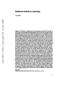
In Fig. 3 the z-scores are presented. In the first line below the graphic there are the laboratory codes, in the second the number of analysed specimens, in the third the squared robust distance and in the forth the corresponding p-values. We used the SLB-method to get qˆ.
Figure 3: z-scores of Zn-concentrations in sewage sludges and corresponding pvalues.
3.3
Choice of materials and distribution of samples
A proficiency test must enable the organiser to see whether there is a general improvement in performance in time. But if the same test material is distributed several times, the participants would become aware of the consensus value after the first round and the credibility of the results in successive rounds would be compromised. Therefore the organiser should distribute also mixtures of samples. As we have seen in the above example the true value of sample S2 could also be determined
INTERLABORATORY STUDIES
263
in an indirect way from samples S6 and S1 , from S7 and S3 , from S8 and S4 and from S9 and S5 . We could organise a future proficiency test in the following way: at each round four specimens P1 , P2 , P3 and P4 are distributed. P1 and P2 are new samples, P3 and P4 are mixtures of P1 and P2 with P0 , where P0 is a specimen from an earlier round with a (only for the organiser) known true value. Then the organiser can evaluate an eventual improvement in performance and even estimate the precision parameters σr and σR at the concentration level of P0 . At a glance, we see the laboratories which have analytical problems for the determination of Zn. Similar graphics for the other elements can be done. As the confidentiality of the results is extremely important in this type of laboratory-performance studies, the organiser distributes to the laboratories only graphics which contain exclusively their own results. Instead of the results of one element of all laboratories (Fig. 3), he distributes graphics which show the results of all elements of a particular laboratory.
4
Conclusions
Monitoring the amount of pollutants in soil, water, air, plants, food, etc. is important nowadays. Analytical tests are required to judge contamination. The fascinating thing about analycal chemical measurements is that they can quantify chemical contents objectively. A drawback is that they suffer from a lack of comparability. It is common knowledge amongst those who practise analysis for trade and commerce that analysts can obtain different results on the same material. Obviously it may not be in their interest to expose this fact. It is in the field of public health and environmental monitoring, where determinand concentrations are often small and where slight differences may be significant, that interlaboratory variation has received most attention. The disturbing thing is the suggestion of unreliability and its possible diffusion to the general public as well as to the governments responsible in cases where important decisions must be made on the basis of chemical measurements. However, the situation is not as bad as it seems. If chemists and statisticians collaborate, try to understand each other’s problems and use realistic models, representative samples, standardised and robust analytical methods, reference materials, interlaboratory tests and good robust statistics, errors can be controlled.
References [1] AMC (1989): Analytical Methods Committee. Robust Statistics Part 2: Interlaboratory Trials. Analyst 114 1699-1702. [2] AMC (1992): Analytical Methods Committee. Proficiency Testing of Analytical Laboratories: Organisation and Statistical Assessment. Analyst 117 97-117. [3] Hampel, F.R. (1985): The Breakdown Points of the Mean Combined With Some Rejection Rules, Technometrics 27 95-107.
264
P. LISCHER
[4] Horwitz, W. Albert, R. (1986): Performance Characteristics of Methods of Analysis Used for Regulatory Purposes. Paper delivered at the PittsburghConference and Exposition, Atlantic City, NJ USA. [5] Horwitz, W. (1988): Protocol for the Design, Conduct and Interpretation of Collaborative Studies. Pure & Appl. Chem. 60(6) 855-864. [6] Huber P. J. (1964): Robust estimation of a location parameter. Ann. Math. Statist. 35 73-101. [7] ISO-5725 (1987): Accuracy (Trueness and Precision) of Test Measurements Part 1: General Principles and Definitions. International Organisation for Standardisation, Geneva, Switzerland. [8] Lischer, P. (1987): Robuste Ringversuchsauswertung. Lebensmittel-Technologie 20 167-172. [9] Mandel, J. (1989): Interlaboratory Testing and Rejection of Observations. Proceedings ISO/REMCO 184. International Organisation for Standardisation, Geneva, Switzerland. [10] Reichenbach, A. (1989): Robuste Methoden f¨ ur die Auswertung von Ringversuchen. Diplomarbeit ETH-Z¨ urich. [11] Rousseeuw, P.J. & Leroy, A.M. (1987): Robust Regression and Outlier Detection. Wiley, New York. [12] Rousseeuw, P.J. & van Zomeren, B.C. (1990): Unmasking multivariate outliers and leverage points. J. Amer. Statist. Assoc. 85 633-639. [13] Rousseeuw, P.J. & Croux, C. (1991): Alternatives to the Median Absolute Deviation, J. Amer. Statist. Assoc. 88 1273-1283. [14] SLB (1989): Schweizerisches Lebensmittelbuch, Kapitel 60. Statistik und Ringversuche. Eidg. Drucksachen- und Materialzentrale, Bern.