Robust Tail Assignment

Robust Tail Assignment vorgelegt von Mgr Ivan Dovica aus Roˇzn ˇava Slowakei Von der Fakultät II – Mathematik und Naturwissenschaften der Technischen Universität Berlin zur Erlangung des akademischen Grades Doktor der Naturwissenschaften – Dr. rer. nat. – genehmigte Dissertation

Vorsitzender: Berichter:

Promotionsausschuss Prof. Dr. Peter Bank Prof. Dr. Dr. h.c. mult. Martin Grötschel Prof. Dr. Ralf Borndörfer

Tag der wissenschaftlichen Aussprache: 28.7.2014

Berlin 2014 D 83

Zusammenfassung Der erste Teil dieser Arbeit behandelt das allgemeine stochastische K¨ urzeste” Wege-Problem“. Gesucht ist der k¨ urzeste Weg in einem Graphen, in dem die Bogenlängen ungewiss und als kontinuierliche Zufallsvariablen definiert sind. Dieses Problem steht im Zentrum verschiedener Anwendungen, vor allem in der robusten Verkehrsplanung, bei der die jeweiligen Wege den Flugzeug-, Zug- oder Busumläufen oder den Dienstplänen der Mitarbeiter entsprechen. Wir schlagen eine neue Lösungsmethode vor, die auf der Diskretisierung von kontinuierlichen Zufallsvariablen basiert. Die Methode ist anwendbar auf jede Klasse von kontinuierlichen Zufallsvariablen. Wir liefern Abschätzungen f¨ ur den Approximationsfehler der diskretisierten Weglängen im Vergleich mit den kontinuierlichen Weglängen. Des Weiteren präsentieren wir theoretische Ergebnisse zum asymptotischen Laufzeitverhalten der Methode. Im zweiten Abschnitt wenden wir diese Methode f¨ ur ein reales Praxisproblem im Flugverkehr an: auf das sogenannte Tail-Assignment-Problem“. Das ” Ziel des Tail-Assignment-Problems“ ist es, die Flugzeugumläufe, d. h. die ” Routen, bestehend aus Flugsegmenten, f¨ ur eine Menge von individuellen Flugzeugen so zu erzeugen, dass eine Menge von gegebenen Fl¨ ugen unter Ber¨ ucksichtigung der Betriebsbedingungen von jedem einzelnen Flugzeug und unter Beachtung der kurz- bis langfristigen individuellen Wartungserfordernisse u ¨berdeckt werden. Wir stellen eine stochastische Formulierung dieses Problems vor und zeigen, wie unsere Methode dieses Problem innerhalb eines Spaltenerzeugungs Frameworks effizient löst. Wir zeigen den Vorteil unseres stochastischen Ansatzes gegen¨ uber dem KPI-Ansatz durch den Vergleich der Propagation der Verspätungen. Es zeigt sich, dass unser Ansatz zu weniger Betriebskosten ohne Erhöhung der Berechnungskomplexität f¨ uhrt. Eine Kernidee unserer Vorgehensweise zur Lösung des Problems der Robusten Optimierung ist das Anpassen des zugrundeliegenden stochastischen Modells auf komplexe Problemstellungen aus der Realität. Wir schlagen ein Modell von Verspätungspropagation vor, das realistisch und gleichzeitig einfach anwendbar, und deswegen ideal f¨ ur Vorhersagen einsetzbar ist. Wir bewerten unsere Ergebnisse durch umfassende Simulationen. Wir zeigen eine erhebliche Verringerung von Ankunftsverspätungen und damit auch von Kosten f¨ ur den Durchschnittsfall sowie f¨ ur eine Vielzahl der Szenarien. Wir evaluieren diese Verbesserung in anderen realistischen Benchmarks durch

Simulation unter Einbeziehung von Gegenmaßnahmen (Rettungsmaßnahmen) und in Szenarien, basierend auf historischen Verspätungsdaten anstelle des stochastischen Modells.

Abstract The first part of this thesis is devoted to the general problem of stochastic shortest path problem. It is about searching for the shortest path in a graph in which arc lengths are uncertain and specified by continuous random variables. This problem is at the core of various applications, especially in robust transportation planning where paths correspond to aircraft, train, or bus rotations, crew duties or rosters, etc. We propose a novel solution method based on a discretisation of random variables which is applicable to any class of continuous random variables. We also give bounds on the approximation error of the discretised path lengths compared to the continuous path lengths. In addition, we provide theoretical results for the computational complexity of this method. In the second part we apply this method to a real world airline transportation problem: the so-called tail assignment problem. The goal of the tail assignment problem is to construct aircraft rotations, routes consisting of flight segments, for a set of individual aircraft in order to cover a set of flight segments (legs) while considering operational constraints of each individual aircraft as well as short- to long-term individual maintenance requirements. We state a stochastic programming formulation of this problem and we show how to solve it efficiently by using our method within a column generation framework. We show the gain of our stochastic approach in comparison to standard KPI in terms of less propagated delay and thus less operational costs without growth of computational complexity. A key point of our complex approach to robust optimisation problem is the fit of the underlying stochastic model with reality. We propose a delay propagation model that is realistic, not overfitted, and can therefore be used for forecasting purposes. We benchmark our results using extensive simulation. We show a significant decrease of arrival delays and thus monetary savings on average as well as in the majority of our disruption scenarios. We confirm these benefits in even more life-like benchmarks as simulation where recovery actions are taken and in scenarios which use historical delays directly instead of the stochastic model.

Acknowledgements I would like to thank Prof. Dr. Dr. h.c. mult. Martin Grötschel for giving me the opportunity to work at ZIB. I am very thankful to Prof. Ralf Borndörfer for his supervision, support, suggestions, and all discussions regarding research and non-research topics. I am also very grateful to Lufthansa Systems team, especially Ivo Nowak and Thomas Schickinger, for their cooperation on the Robust Tail Assignment project and fruitful discussions on meetings. I would like to thank Carlos and Dung for proof-reading parts of my thesis; Miˇska and Miloˇs for grammar corrections; and Benjamin, Thomas, Marcus, and Ambros for help with translations to German during my time at ZIB. Special thanks goes to Bettina for helping me with many day-to-day problems that often seemed to be harder than research itself. I would like to thank also all colleagues at ZIB for creating great working atmosphere that made my time at Berlin so great. Last but not least I want to thank my wife Tereza and my parents for their endless patience and support.

Contents Introduction Contribution . . . . . . . . . . . . . . . . . . . . . . . . . . . . . . Thesis Outline . . . . . . . . . . . . . . . . . . . . . . . . . . . . . 1 The 1.1 1.2 1.3 1.4

1.5

Stochastic Shortest Path Problem Problem Definition . . . . . . . . . . . . . . . Labelling Algorithm . . . . . . . . . . . . . . Discretisation of Continuous RandomVariables Discretised Labelling Algorithm . . . . . . . . 1.4.1 Expectation . . . . . . . . . . . . . . . 1.4.2 Dominance . . . . . . . . . . . . . . . 1.4.3 Convolution . . . . . . . . . . . . . . . Approximation Error . . . . . . . . . . . . . .

2 Introduction To Airline Planning 2.1 Schedule Generation . . . . . . . 2.2 Fleet Assignment . . . . . . . . . 2.3 Maintenance Routing . . . . . . . 2.4 Crew Planning . . . . . . . . . . 2.5 Tail Assignment . . . . . . . . . . 2.6 Recovery . . . . . . . . . . . . . . 2.7 Integration . . . . . . . . . . . . . 2.8 Robustness in Airline Planning .

1 3 4

. . . . . . . .

. . . . . . . .

. . . . . . . .

. . . . . . . .

. . . . . . . .

. . . . . . . .

. . . . . . . .

. . . . . . . .

. . . . . . . .

7 8 10 14 16 17 17 18 21

. . . . . . . .

. . . . . . . .

. . . . . . . .

. . . . . . . .

. . . . . . . .

. . . . . . . .

. . . . . . . .

. . . . . . . .

. . . . . . . .

. . . . . . . .

. . . . . . . .

. . . . . . . .

. . . . . . . .

. . . . . . . .

. . . . . . . .

. . . . . . . .

25 26 26 27 27 28 29 30 31

3 Delay Propagation 3.1 Motivation . . . . . . . . . . . . . . 3.2 Delay Propagation in the Literature 3.3 The Model of Airline Operations . 3.3.1 Crew Operations . . . . . .

. . . .

. . . .

. . . .

. . . .

. . . .

. . . .

. . . .

. . . .

. . . .

. . . .

. . . .

. . . .

. . . .

. . . .

. . . .

37 38 40 41 43

i

3.4

3.5

3.6

3.7

Rotational Delay Propagation . . . . . . . . . . . 3.4.1 Formal Computation of Propagated Delays 3.4.2 Implementation . . . . . . . . . . . . . . . Non-rotational Delay Propagation . . . . . . . . . 3.5.1 Formal Computation of Propagated Delays 3.5.2 Implementation . . . . . . . . . . . . . . . 3.5.3 Dependency of Random Variables . . . . . 3.5.4 Dependency of Delay on Other Rotations . Performance and Accuracy . . . . . . . . . . . . . 3.6.1 Asymptotic Complexity . . . . . . . . . . 3.6.2 Speed-up . . . . . . . . . . . . . . . . . . . 3.6.3 Computational Results . . . . . . . . . . . 3.6.4 Conclusions . . . . . . . . . . . . . . . . . Summary . . . . . . . . . . . . . . . . . . . . . .

. . . . . . . . . . . . . .

4 The Robust Tail Assignment Problem 4.1 Problem Definition . . . . . . . . . . . . . . . . . . 4.2 Stochastic Programming Model RoTA . . . . . . . 4.2.1 Column Generation Approach . . . . . . . . 4.2.2 Pricing Problem for RoTA . . . . . . . . . . 4.3 Two-stage Stochastic Programming Model NoRoTA 4.3.1 Pricing Problem for NoRoTA . . . . . . . . 4.3.2 Approximate Column Generation Approach 5 Stochastic Model 5.1 Model Overview . . . . . . . . . . . . . . . . . . . 5.1.1 Stochastic Models in Airline Optimisation 5.1.2 Structure of the Model . . . . . . . . . . . 5.2 Historical Data . . . . . . . . . . . . . . . . . . . 5.2.1 Data Filtering . . . . . . . . . . . . . . . . 5.3 Methodology . . . . . . . . . . . . . . . . . . . . 5.4 Primary Gate Delays . . . . . . . . . . . . . . . . 5.4.1 The Probability of Primary Gate Delays . 5.4.2 The Length of Primary Gate Delays . . . . 5.4.3 Summary . . . . . . . . . . . . . . . . . . 5.5 Block Time Deviation . . . . . . . . . . . . . . . 5.5.1 Summary . . . . . . . . . . . . . . . . . . 5.6 Minimum Ground Time and Minimum Sit Time . 5.7 Properties of the Stochastic Model . . . . . . . . ii

. . . . . . . . . . . . . .

. . . . . . . . . . . . . .

. . . . . . .

. . . . . . . . . . . . . .

. . . . . . . . . . . . . .

. . . . . . .

. . . . . . . . . . . . . .

. . . . . . . . . . . . . .

. . . . . . .

. . . . . . . . . . . . . .

. . . . . . . . . . . . . .

. . . . . . .

. . . . . . . . . . . . . .

. . . . . . . . . . . . . .

. . . . . . .

. . . . . . . . . . . . . .

. . . . . . . . . . . . . .

44 44 45 53 53 56 56 59 61 61 62 65 70 70

. . . . . . .

71 71 73 74 75 81 85 89

. . . . . . . . . . . . . .

93 94 94 95 96 97 99 101 102 103 108 108 111 111 112

5.8

6 Ops 6.1 6.2 6.3 6.4 6.5 6.6

Model Justification . . . . . . . . . . . . . . . . . . . . . . . . 114 5.8.1 Stability of Parameters . . . . . . . . . . . . . . . . . . 114 5.8.2 Proof of Concept . . . . . . . . . . . . . . . . . . . . . 118 Simulator Overview of Simulation Frameworks Structure of the Ops Simulator . . Simulation Module . . . . . . . . . Cost Model . . . . . . . . . . . . . Recovery in the Ops Simulator . . . 6.5.1 Netline/Ops Solver xOPT . Visualisation . . . . . . . . . . . . .

. . . . . . .

. . . . . . .

. . . . . . .

. . . . . . .

7 Computational Results 7.1 Overview . . . . . . . . . . . . . . . . . . . 7.1.1 Testing Methodology . . . . . . . . 7.1.2 KPI Objective (ORC) . . . . . . . 7.1.3 Instances . . . . . . . . . . . . . . 7.2 Performance of the RoTA Model . . . . . . 7.3 Performance of the NoRoTA Model . . . . 7.4 Impact . . . . . . . . . . . . . . . . . . . . 7.4.1 Average Savings . . . . . . . . . . . 7.4.2 Analysis Of Individual Simulations 7.5 Performance under Recovery . . . . . . . . 7.6 Proof of Concept . . . . . . . . . . . . . . 7.6.1 Stochastic Model . . . . . . . . . .

. . . . . . .

. . . . . . . . . . . .

. . . . . . .

. . . . . . . . . . . .

. . . . . . .

. . . . . . . . . . . .

. . . . . . .

. . . . . . . . . . . .

. . . . . . .

. . . . . . . . . . . .

. . . . . . .

. . . . . . . . . . . .

. . . . . . .

. . . . . . . . . . . .

. . . . . . .

. . . . . . . . . . . .

. . . . . . .

. . . . . . . . . . . .

. . . . . . .

121 . 122 . 123 . 124 . 125 . 128 . 128 . 130

. . . . . . . . . . . .

133 . 134 . 134 . 135 . 136 . 138 . 139 . 141 . 141 . 143 . 147 . 152 . 152

8 Perspectives

155

Bibliography

157

iii

iv

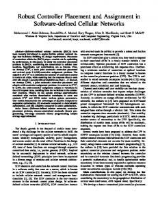
Introduction Eurocontrol STATFOR (2010) [52] reports that in the most-likely future scenario European airports will serve about 80% more flight legs in 2030 than in 2009. This corresponds to an average annual growth of 2.8% while many European airports are nowadays already reaching their capacity limits. Traffic growth will increase congestion on airports and thus increase delay generation. Highly congested airports and airspaces are more likely to cause delays and are less flexible in accommodating unexpected traffic (caused by delayed legs). This is even more true as slack times in aircraft and staff utilization have been reduced by continuous advances in the optimisation techniques. All these factors contribute to delay increase, annoy, and shoot up operational costs of airlines. Figure 1 demonstrates this fact on data derived from annual reports of Central Office for Data Analysis (CODA) for the years 2003 to 2012, see CODA [35]. We observe correlation between air traffic volume and the share of delayed legs on arrival. After years of traffic and delay growth, there is a steep decrease during the economical crisis in 2008 and 2009. The discrepancy in the 2010 and 2011 data development is caused by an extraordinary growth of delays in 2010 due to the ash cloud caused by the volcano eruption on Iceland and poor weather. Clearly, delays are causing huge financial losses to airlines. Therefore, they are subject of massive investigation with the goal to get delays and financial impacts under control. Ball et al. (2010) [11] estimate the total cost of all US air transportation delays in 2007 at $32.9 billion, of which direct airline costs are estimated at $8.3 billion and the value of passengers’ lost time at $16.7 billion. Based on European data, Cook, Tanner & Anderson (2004) 1

6 4 2 0 −2 −4

annual change

−6

traffic volume (in %) delayed arrivals (in %age points) 2004

2005

2006

2007

2008

2009

2010

2011

2012

Figure 1: Comparison of the annual growth of air traffic volume (measured by number of operated legs) on European airports and the increase of legs delayed at least 15 minutes on arrival (measured in absolute changes in percent). [38] estimate the average cost of one minute of delay longer than 15 minutes at 72 e. These figures have consequences for airline scheduling. The growth of operational costs in comparison to the decrease in scheduled costs led airlines to rethink their perception of the “ideal schedule”. They now ask for schedules that are cost effective in the real operation, under delays, and not only “on the paper”. Such schedules are called robust schedules. The last decade brought various approaches to robust scheduling in all planning stages from the fleet assignment to tail assignment. The easiest way, from a mathematical point of view, is to improve robustness by incorporating some additional robustness measure, called key performance indicator (KPI), into the current optimisation objectives. KPIs assure favourable properties of 2

the schedule that are supposed to improve its performance under disruptions. Clearly, different scheduling problems desire different KPIs. Typical KPIs are for example, minimising the total buffer for each rotation, stipulating some threshold ground buffer before each leg, avoiding visits of single aircraft on certain airports too often during one day, minimising the number of aircraft types serving each hub, avoiding crews changing the aircraft etc. KPI approaches are typically simple to implement. Their disadvantage is that there is no clear connection between the KPI and increased leg punctuality, decreased propagated delay, or additional expenses. Hence, the benefit of a KPI approach is disputable or easily be negative. In order to achieve better results on a solid scientific basis, one has to come up with more accurate and rigorous models which have to cope with disruptions directly and which asses their impact directly. It is very important to properly model disruptions and their impact on the whole network. Unfortunately, the computation of delay propagation is difficult even for small sized problems. Approaches from the literature are too slow for practical applications, have disputable accuracy of results, or apply only under special conditions that are not fulfilled in practice.

Contribution In this thesis, we propose a novel method to compute the length of a path in a graph whose arc lengths are subject to uncertainty and specified by random variables. This stochastic shortest path problem is widely applicable in transportation planning problems in which uncertainties of transfer durations. We focus on a concrete application in airline planning, namely, the tail assignment problem. We consider the optimisation of natural objectives such as the expected arrival delay, the probability of delay propagation, and the expected additional airline costs. The basis of this method is an approximation of continuous functions, representing probability density functions of continuous random variables, by step functions. This is kind of discretisation. We provide an effective and accurate implementation of operations that are required for computing of delay propagations in an airline network. Furthermore, the discretisation is applicable to any class of continuous distributions. 3

Therefore, the method can be applied to any suitable problem independently of the choice of the stochastic model. It also ensures a high accuracy of the underlying stochastic model. Our discretisation method is particularly suited for problems which are solved by the column generation framework. We demonstrate its application at the example of the tail assignment problem, which deals with the generation of aircraft rotations a few days before the day of operation. We formulate a stochastic programming model for the robust tail assignment problem in which we minimise the total probability of delay propagation. Due to the discretisation method we are able to solve this model effectively by a deterministic algorithm. Furthermore, we develop a simple but precise stochastic model of airline operations. The model has only very few parameters. It therefore can be calibrated using rather small data sets. We pay particular attention to an assessment of the benefits of our approach under as realistic conditions as possible. To this purpose, we develop a framework for simulation and evaluation of aircraft schedules. Our simulator allows an evaluation of schedules under randomly generated disruptions sampled using our stochastic model. The simulator is able to perform recovery actions; this brings simulation even closer to reality. Finally, we use the simulator for the visualisation of schedules and simulation results. Our results were awarded with the Anna Valicek Award 2010 of the Airline Group of the International Federation of Operations Research Societies (AGIFORS) which recognises original and innovative research in the application of operations research to airline and/or airline related business problems.

Thesis Outline In Chapter 1 we investigate a classical problem of the graph theory, the shortest path problem. It appears in many applications in transportation. We formulate a stochastic version of this problem in which arcs have stochastic lengths. We call this problem the stochastic shortest path problem. In order to solve the stochastic shortest path problem, we propose a discretisation method for continuous random variables. We study algorithmic 4

computation of operations such as convolution, expectation, and stochastic dominance over discretised random variables. Furthermore, we provide a theoretical bound on the approximation error of the method. Chapters 2-7 are dedicated to the application of the discretisation method to robust airline planning. Chapter 2, we survey current planning practices of airlines and give a survey of the field of robust airline planning. In Chapter 3, we study how delay propagates in airline networks. We formalise this process in a mathematical model and we show how to apply the discretisation method to the computation of the delay propagation in this model. We extend the formal definition of the method from Chapter 1, which applies to general graphs, in order to make it applicable to airline networks. We also provide implementations of all stochastic operations required. The efficiency of the method is demonstrated in a computational study which demonstrates low computation times and high accuracy when applied to the computation of delay propagation in realistic aircraft rotations. In Chapter 4 we formulate a robust version of the tail assignment problem. We give a stochastic programming formulation which minimises the probability of delay propagation across the network. In order to solve the model, we use results from the previous chapter. Namely, the probability of delay propagation, and thus the computation of the propagated delay, along aircraft rotation is required in the pricing problem of a column generation approach. Furthermore, we state a two-stage stochastic programming model in order to solve the robust tail assignment problem with consideration of non-rotational delay propagation. Such delays are caused, for example, by crew changing the aircraft, transferring passengers, or cargo. We propose an approximate column generation algorithm for solving this problem. The algorithm, again, relies on the discretisation method in solving the pricing problem. In Chapter 5, we present details of our stochastic model of primary delay generation. The model is derived from historical operational data. It focuses simplicity and plausibility. The model is used in our optimisation approach as well as in our simulator. Chapter 6 documents the simulation and visualisation tool Ops Simulator. The simulator is an important part of this work since it allows to estimate the practical gain of our approach over KPI methods in an lifelike environment. 5

In Chapter 7, we present computational results for real world instances of the robust tail assignment problem. Using the Ops Simulator, we document a genuine decrease in operational costs.

6

Chapter 1 The Stochastic Shortest Path Problem The goal of this chapter is to present an algorithm for solving the stochastic shortest path problem. The stochastic shortest path problem can be seen as a generalisation of the shortest path problem where arc lengths are random variables. First in Section 1.1, we give an overview of known formulations of the stochastic shortest path problem from the literature and we discuss their algorithmic complexity. We state a general formulation of the problem. That is, we do not take any assumptions on the arc length distributions and we assume the cost function may be any non-decreasing function. In Section 1.2, we propose a labelling algorithm for solving this formulation. An implementation of the algorithm relies on a novel discretisation technique for representation of continuous random variables which is presented in Section 1.3. In Section 1.4, we define all essential operations over discretised random variables required for implementation of labelling algorithm. Moreover in Section 1.5, we estimate an approximation error of distribution of the path length introduced through employment of the discretisation technique. Discretisation method plays central role in this work. In Chapter 3, we provide an extension of our discretisation method for computation of the propagated delay along aircraft rotations and we provide details about its application. Such extension is then applied for solving the robust tail assignment, which is introduced in Chapter 4. 7

1.1

Problem Definition

The shortest path problem is one of the most important problems in Graph Theory. Many practical problems can be formulated as the shortest path problem or contain this problem as a sub-problem. Several efficient algorithms have been proposed to solve this problem. However, recent advances in applied mathematics ask for more realistic modelling of practical problems which lead to generalisations of this problem towards reflecting uncertainty of the parameters. Input data for the mathematical models are often noisy, unknown, or have stochastic nature. Such data, thus, have to be predicted by random variables. For example, travel time between two cities depends on congestion of the road, which may be predicted by a random variable. In the context of the shortest path problem this idea leads to the definition of the stochastic shortest path problem where arc lengths, representing distances between cities, are random variables. Formally, the stochastic shortest path problem can be stated as follows. Let G = (V, E) be a graph with set of vertices V , arcs E, and two distinguished vertices s, t ∈ V . Arc lengths Xe , e ∈ E are real-valued random variables. We are looking for the shortest st-path in the graph. So defined stochastic shortest path problem finds application in many practical problems. For all we mention application in public transportation planning, see for instance Borndörfer et al. (2010) [26]. In context of the stochastic shortest path problem, definition of the optimal (or ”‘shortest”’) path is disputable and depends on specific application. Moreover, the objective function has impact on solvability of the problem. The literature proposes various formulations of the problem and complexity results for the formulations. The most natural seems to be to minimise expected length of the path. Although let us have, in the aforementioned example, given some deadline for arriving to destination city (or vertex t). Minimisation of expected travel duration (or path length) does not make sense since we rather want to find a path which gets us to destination city (or vertex t) most likely before the deadline. Frank (1969) [56] proposes this optimality criterion, that is, the objective function is to identify the path with the highest probability to have weight smaller than some given threshold. Another optimality criterion 8

propose Sigal, Pritsker & Solberg (1980) [98]. They search for the path that is the shortest of all paths with the highest probability. Most optimality criteria can be formally defined by some cost function w defined on the path length. Then the goal is to minimise expected value of the cost function. Whether the problem can be solved efficiently or not depends on the cost function. Nikolova, Brand & Karger (2006) [85] prove that it is NP-hard to find the path with the lowest expected cost for general cost functions with a global minimum. On the other hand, there are known cases when the problem is efficiently solvable. For example, minimisation of expectation of linear cost function is efficiently solvable since it holds E (w (Xe1 + Xe2 )) = E (w (Xe1 )) + E (w (Xe2 )) . Thus, one can replace arc lengths Xe by their expected costs E (w (Xe )) and solve the corresponding deterministic shortest path problem by standard algorithms. Efficient dynamic programming algorithm is also applicable for the exponential cost function, see Eiger, Mirchandani & Soroush (1985) [49] and Loui (1983) [80]. Eiger, Mirchandani & Soroush (1985) [49] prove validity of Bellman’s Principle of Optimality for the exponential cost function. They show that if expected cost of some path p1sv from s to v is smaller than of path p2sv , then the same holds for any extensions of these paths. This follows from non-negativity of E (w (Xe )) and from the fact that for exponential w E w Xp1sv + Xe = E w Xp1sv E (w (Xe )) .

We consider the problem in very general setting where the expected value of some non-decreasing cost function is minimised. Such formulation includes many of aforementioned formulations as a special case. In order to avoid negative cycles in the graph, we restrict ourselves to directed acyclic graphs. This formulation is also satisfactory for the application of the problem in following chapters. Another possibility how to avoid negative cycles is to require non-negative edge lengths and positive cost function instead. Definition 1.1.4 states studied problem. Definition 1.1.1. Given a probability space (Ω, F, P ) where Ω denotes a sample space, F ⊂ 2Ω is a set of events, and P : F → [0, 1] is a probability measure; a random variable X is a measurable function X : Ω → R+ 9

v Definition 1.1.2. The probability density function of a random variable X is the function fX : R → [0, 1] where Z b P [a ≤ X ≤ b] = fX (x)dx. a

Definition 1.1.3. The cumulative density function of a random variable X is the function FX : R → [0, 1] where FX (x) = P [X ≤ x]. Definition 1.1.4 (Stochastic Shortest Path Problem). Let G = (V, E) be an acyclic directed graph with set of vertices V , set of arcs E, and two distinguished vertices s, t ∈ V . Given real-valued independent continuous random variables Xe , e ∈ E, of arc lengths with known probability density functions, and non-decreasing cost function w, we want to find the st-path p∗st with the smallest expected cost p∗st = min E (w (Xp )) p∈Pst P where Xp = e∈p Xe and Pst is the set of all directed paths p from s to t.

1.2

Labelling Algorithm

Loui (1983) [80] proves that the formulation of the stochastic shortest path problem, where expectation of non-decreasing cost function is minimised, cannot be efficiently solved since Bellman’s Principle of Optimality does not hold. This principle is inevitable assumption for development of an efficient dynamic programming algorithm. Loui (1983) [80], therefore, proposes the labelling algorithm for solving two special cases of the stochastic shortest path problem. The first one with the quadratic cost function, and the second with arc length distributions closed under convolution and uniquely determined by the first two moments. In both cases the cost of every path length can be computed easily from arc length distributions and is determined by the first two moments. Thus, the first and the second moment of the path length are used as the labels in the labelling algorithm. Murthy & Sarkar (1996) [84] enhance the performance 10

Algorithm 1: Labelling algorithm for solving the stochastic shortest path problem Input : Digraph G = (V, E) with random variables for arc lengths Xe , e ∈ E, non-decreasing cost function w, and two vertices s, t ∈ V Output: st-path with the smallest expected cost 1 Ls := {(0)}; 2 Lv := ∅ for all v ∈ V \ {s}; 3 sort V topologically as v1 , . . . , vj = s, . . . , vk = t, . . . , vn ; 4 for i := j to k − 1 do 5 u := vi ; 6 remove all dominated labels from Lu by Dominance Rule 1.2.1; 7 for (u, v) ∈ E do 8 for (Xpsu ) ∈ Lu do 9 Xpsv := Xpsu + Xuv ; 10 Lv := Lv ∪ {Xpsv }; 11

return arg minpst :Xpst ∈Lt E(w(Xpst ));

of the labelling algorithm for the concave quadratic cost function by the pruning technique what decreases number of enumerated labels. In our problem formulation, we do not take any assumptions on the arcs length distributions and on the cost function. Thus, we have to introduce more general labels and dominance rule for the labelling algorithm. Moreover, we have to tackle a problem of summing general continuous random variables in order to derive distributions of path lengths. Our approach is described by Algorithm 1. We propose the labelling algorithm that uses full description of the path distribution in the labels. We assign sets Lv of labels Xpsv to all vertices. Each label set Lv stores probability distribution functions of the length of paths psv from vertex s to vertex v. We guarantee finiteness of the algorithm by examination of the vertices in topological order. We recall that topological order is a linear order of vertices with no backward arcs. In order to save some running time over pure enumeration, we prune labels of all dominated paths in Step (6) by Dominance Rule 1.2.1. Correctness of the dominance rule proves Theorem 1.2.2. 11

Definition 1.2.1 (Stochastic Dominance Rule). Let p1 and p2 be two svp1 p2 p1 and F p2 cumupaths with lengths Xsv and Xsv , respectively. Denote FXsv Xsv p1 p2 lative density function of random variable Xsv and Xsv , respectively. We say, that path p2 dominates path p1 if for all x ∈ R p1 (x) ≤ F p2 (x) . FXsv Xsv

Theorem 1.2.2 (Correctness of Dominance Rule). Let w be non-decreasing cost function, and let us have two sv-paths p1 and p2 with lengths represented p1 p2 p1 and F p2 cuby random variables Xsv and Xsv , respectively. Denote FXsv Xsv p1 p2 mulative density functions of Xsv and Xsv , respectively. If for all x ∈ R p1 (x) ≤ F p2 (x) , FXsv Xsv

then path p1 is suboptimal, that is, it is not part of any st-path with the smallest expected cost. Proof. Let us denote p3 any vt-path. First, we show that if p2 dominates p1 , then for extension of paths p1 and p2 along path p3 to vertex t holds FX p1 +p3 (x) ≤ FX p2 +p3 (x), for all x ∈ R. In other words, any extension of st st path p1 is dominated by the same extension of path p2 . Then we show that every dominated path is suboptimal, that is, p1 (x) ≤ F p2 (x) , ∀x ∈ R FXsv Xsv

⇒

p1 p2 E (w (Xsv )) ≥ E (w (Xsv )) .

These two facts prove that there is always extension of p2 that has lower costs than corresponding extension of p1 and therefore path p1 can be pruned. p3 Let us pick some vt-path and denote Xvt random variable of the length of this path, that is, p3 Xvt =

X

Xe .

e∈p3

p1 +p3 p3 p2 +p3 p3 p1 p2 Then Xst = Xsv + Xvt and Xst = Xsv + Xvt . From Definition 1.1.4, we know that Xe , for all e ∈ E are independent random variables and since p3 p1 p2 all paths in the graph are acyclic, Xvt is independent of Xsv and Xsv . The

12

cumulative density function of the sum of two independent random variables can be computed by the following convolution integral Z ∞ FX+Y (t) = FX (x)fY (t − x)dx. −∞

Therefore, for all t ∈ R holds p p p2 p FXsv +Xvt3 (t) − FXsv1 +Xvt3 (t) =

− =

Z

∞

Z −∞ ∞ Z−∞ ∞

−∞

p2 (x)f p3 (t − x)dx FXsv Xvt

p1 (x)f p3 (t − x)dx = FXsv Xvt

p2 (x) − F p1 (x) f p3 (t − x)dx ≥ 0. FXsv Xsv Xvt

p3 and dominance where the last inequality follows from non-negativity of fXvt of p1 by p2 . This concludes the first part of the proof.

Let us define function u : R → R such that p1 (u (x)) = F p2 (x) . FXsv Xsv p1 and F p2 are increasing and Without loss of generality we assume that FXsv Xsv continuous functions. Together with the fact that p2 dominates p1 it is easy to see that u is non-decreasing function. Expectation of some random variable can be defined as Z ∞ Z 1 E(w(X)) = w(x)f (x)dx = w(x)dF (x).

−∞

0

Hence, p1 E (w (Xsv ))

=

Z

1

1

p1 (u(x)) w(u(x))dFXsv Z 1 Z 1 p p p2 (x) = E (w (X 2 )) . = w(u(x))dFXsv2 (x) ≥ w(x)dFXsv sv

0

p1 (x) = w(x)dFXsv

Z

0

0

0

Notice that the inequality follows from the fact that functions u and w are both non-decreasing. Unfortunately, Algorithm 1, as stated, is only of theoretical relevance. In order to make it implementable in practise, we have to introduce 13

• compact representation of continuous random variables, • computation of the distribution of the path length (Step 9), • evaluation of dominance rule (Step 6), • computation of expected cost of the path (Step 11). In particular, computation of sum of the random variables, which leads to evaluation of convolution integral, is difficult and widely studied problem. To solve this problem, we propose a novel approach to computing convolution integral by discretising random variables in the next section.

1.3

Discretisation of Continuous Random Variables

The core of our approach lies in the approximation of probability density functions of continuous random variables by the step functions, which are piecewise constant functions, with finitely many pieces. This method is applicable to every distribution class of random variables with known cumulative density function. The step functions can be represented by finite number of real values which simplifies representation of random variable in the computer memory. In Section 1.4, we show that such representation allows very efficient way to compute convolution integral as well. Moreover, the technique can be repeatedly used to arbitrarily many summands since result of the convolution can be easily approximated by the step function and thus used in next convolution. The method allows analysis of the approximation error, which is addressed in Section 1.5. We approximate the probability density function fX of continuous random variable X by step function fX k with constant step size k. We choose step values in a way that the cumulated probability of each step equals cumulated probability of fX on this interval. This also assures that fX k integrates to one on the domain. Therefore function fX k can be seen as probability density function of a continuous random variable and we denote the random variable with probability density function fX k as X k . 14

0.08 probability 0.04 0.06 0.02 0.00

20

30

40 minutes

50

60

Figure 1.1: Discretised probability density function of a continuous random variable. For every step end point ik, i ∈ Z also holds FX (ik) = FX k (ik) where FX and FX k are cumulative density functions. For illustrative example of a discretised probability density function see Figure 1.1. Most of distributions have unbounded support mathbbR or R+ . In order to be able to represent the probability density function by a finite number of steps, we restrict the support, on which the function gains positive values, to a bounded interval. Clearly, fX (x) > ε for each ε > 0 holds on some bounded support. Denote xl (ε) lower bound and xu (ε) upper bound of this support xl (ε) = max {x ∈ R | fX (y) < ε, ∀y < x} , xu (ε) = min {x ∈ R | fX (y) < ε, ∀y > x} .

(1.1)

Note that we pick ε very small and fixed. Such bounding of the support is not harming the performance of the method because of limited accuracy of the representation of real numbers in the computer where the non-zero values smaller than some very small threshold values are rounded to zero. We assume that tails of the distribution, which are cut off after we round values smaller than ε to zero, have cumulated probability less than δ(ε) > 0 15

where δ(ε) is still very small. Therefore, we assume that Z xu (ε) f (x)dx = 1. xl (ε)

The following definition formalises described discretisation process. Definition 1.3.1 (Discretised Random Variable). Let X be a continuous random variable with probability density function fX and cumulative density function FX . We denote by Xk the continuous random variable with probability density function fX k which is the step function with step size k and fX k is defined as  αX k , for x ∈ (k (i − 1) , ki] , i = l k , . . . , u k , X X i fX k (x) = (1.2) 0, else, where k

αiX =

R ki

k(i−1)

fX (x)dx k

=

FX (ki) − FX (k(i − 1)) , k

i = lX k , . . . , uX k . (1.3)

Lower and upper bound on non-zero steps are defined as lX k = ⌊xl (ε)/k⌋ and uX k = ⌈xu (ε)/k⌉. We refer to Xk as discretised continuous random variable. Notice that lX k and uX k also depend on ε thus, notion lX k (ε) and uX k (ε) would be more appropriate. Nevertheless, we prefer the simpler notion when no confusion can arise.

1.4

Discretised Labelling Algorithm

Now we show how to implement Algorithm 1 with employment of discretised random variables. We refer to such implementation as Discretised Labelling Algorithm. We start with showing how to compute expected cost of the path for Step (11), and evaluation of dominance rule in Step (6). In the end of this section, we show the implementation of the convolution of discretised random variables which is necessary operation for implementation of Step (9). 16

1.4.1

Expectation

Expected cost of X is for some real valued integrable cost function w defined Z ∞ E(w(X)) = w(x)fX (x)dx. −∞

When using X k instead of X, computation of expectation is straightforward because it reduces to the sum k

E(w(X )) =

uX k X

k αiX

i=lX k

Z

ki

w(x)dx. ki−k

R In case there is no analytical description of w(x)dx given, one can approximate the value of the function by some quadrature rule for numerical integration as trapezoidal rule Z

ki

w(x)dx ≈ k ki−k

w(ki − k) + w(ki) 2

or Simpson’s rule Z

ki

w(x)dx ≈ k ki−k

w(ki − k) + 4w(ki − k2 ) + w(ki) . 6

For short survey on this topic see Smyth (1998) [102].

1.4.2

Dominance

The cumulative density function of the discretised continuous random variable is a piecewise linear function with equally spaced segment end-points. Hence, to implement Dominance Rule 1.2.1 for X1k and X2k it suffices to check dominance at segment end-points what is done by the evaluation of sums j X

kfX1k (ik) ≤

i=min{lX k ,lX k } 1

j X

kfX2k (ik),

i=min{lX k ,lX k }

2

1

2

for each j = min{lX1k , lX2k }, min{lX1k , lX2k } + 1, . . . , max{uX1k , uX2k }. 17

1.4.3

Convolution

Let X and Y be two independent random variables with integrable probability density functions fX and fY , and let Z by their sum Z = X + Y . Probability density function fZ of Z can be computed as the following convolution integral Z ∞ fZ (t) = fX (x)fY (t − x)dx. (1.4) −∞

Since we do not take any assumptions on distribution classes and parameters of random variables we can compute this integral numerically; analytical evaluation is unfortunately possible only in special cases. Various approaches to numerical computation of integrals can be found in the literature. See Krommer & Ueberhuber (1994) [73], Krommer & Ueberhuber (1987) [72], and Srivastava & Buschman (1992) [105] for an overview of various methods for numerical integration. The primal focus of these methods is to compute a single integral. Our application, however, requires method for finding function fZ rather than a value in single point fZ (t). Besides, effective repeated employment of the method is one of the key properties which we require from the integration method. Therefore, resulting function fZ has to fulfil assumptions taken by the method on initially integrated functions fX and fY so that fZ can be used for further computation. Moreover, some methods are computationally intensive, which makes their application thousands of times during a single optimisation prohibitive. Fan, Kalaba & Moore II (2005) [53] tackle the problem of evaluation of convolution along a path by application of Laplace transforms. Badinelli (1996) [9] provides computational study of various methods using approximation by orthogonal polynomials. He compares the accuracy of the methods with respect to the number of approximation points. Another approach presents Frank (1969) [56], where he proposes a Monte Carlo simulation method to estimate the probability density function of the path length. Clearly, convolution of discrete random variables is much easier to compute since it reduces to evaluation of sums. This idea was used by Dodin (1985) [43] where he discretises probability density functions to finite number of values, which are computed by solving the system of non-linear equations. Obtained discrete distributions are then used for further computations. In 18

other words, he approximates continuous random variables by discrete random variables. We also use the advantage of working rather with sums instead of integrals. Unlike Dodin (1985) [43], we still work with continuous random variables. Discretisation introduced in the previous section allows us to compute convolution as easily as for discrete random variables while still working with continuous random variables. Let X and Y be continuous random variables and X k and Y k be their respective discretisations with identical step size k. Notice that the variables does not necessarily have identical upper and lower step bounds lX k , lY k , and uX k , uY k but the points separating the steps in each function are the same equal, namely, integers divisible by k. In the first step, instead of computing probability density function fZ of Z = X + Y , by evaluating Integral (1.4), we compute Z¯ k = X k + Y k . As we show, probability density function of Z¯ k is not a step function. Therefore in the second step, we approximate Z¯ k by Z k with fZ k as step function. In order to compute fZ¯k , we have to evaluate integral fZ¯k (t) =

Z

∞

fX k (x)fY k (t − x)dx.

(1.5)

−∞

Observation 1.4.1. Function fZ¯k is piecewise linear function with line segments end-points ik where i ∈ {lZ¯k , lZ¯k + 1, . . . , uZ¯k } = {lX k + lY k − 2, lX k + lY k − 1, . . . , uX k + uY k }. and fZ¯k (x) = 0 on intervals (−∞, k (lX k + lY k − 2)) and (k (uX k + uY k ) , ∞). Moreover, function values in the line segment end-points can be computed as

fZ¯k (ik) =

∞ X

j=−∞

min{uX k ,i+1−lY k } Xk

k

X

Y = kαj αi−j+1

k

k

Y kαjX αi−j+1 .

(1.6)

j=max{lX k ,i+1−uY k }

Let us explain this fact. Since both density functions have equal step size, we can rewrite Integral (1.5) for any ik as the sum of integrals over individual 19

steps fZ¯k (ik) = = =

Z

∞

fX k (x)fY k (ik − x)dx

−∞ ∞ X

k

Z

fX k (jk − y)fY k (ik − jk + y)dy

j=−∞ 0 ∞ Z k X j=−∞

k Yk αjX αi−j+1 dy

0

=

∞ X

k

k

Y kαjX αi−j+1 .

(1.7)

j=−∞

where the second equation is only reformulation following from the definition of discretised random variables, see Definition 1.3.1. Notice that, for simplik fication, we consider αiX to be defined also for i < lX k and i > uX k and k clearly, αiX = 0 in such situation. k

k

Y Clearly, summand j is non-zero only if αjX is non-zero and αi−j+1 is non-zero which holds only for j such that

l X k ≤ j ≤ uX k , l Y k ≤ i − j + 1 ≤ uY k . It is also easy to see that for i ≤ lX k + lY k − 2 and for i ≥ uX k + uY k there is no such j and therefore all summands equal zero as well as fZ¯k (ik). Now, we approximate resulting probability density function by the step function. We approximate fZ¯k by step function fZ k so that the mass of the function on each line segment is preserved. Therefore, ( k αiZ , for x ∈ (k(i − 1), ki], i = lZ k , . . . , uZ k , fZ k (x) = 0, else, where k

αiZ =

fZ¯k (k(i − 1)) + fZ¯k (ki) , 2

i = l Z k , . . . , uZ k ,

(1.8)

and lZ k = lZ¯k + 1 and uZ k = uZ¯k . Notice that this approach preserves properties of probability density functions for fZ k because fZ k is non-negative function and Z ku k Z fZ k (x)dx = 1 klZ k

under assumption that fX k and fY k are also probability density functions. 20

1.5

Approximation Error

In the previous section we showed how to implement Algorithm 1 by using discretised random variables. Discretisation itself introduces an approximation error in the representation of probability density function of the random variables. By the approximation error, we understand absolute maximal discrepancy between true value of the function and the represented value. Along the path search, as the sum of random variables is evaluated, the initial approximation error is amplified. It is, therefore, important to asses the growth of approximation error with increasing amount of summed random variables. Now, let us prove that the approximation error of the implementation is very small. Actually, we show that the error is linear in terms of number of convoluted random variables and discretisation step size. Theorem 1.5.1. Let Xi for i = 1, . . . , n be continuous random variables and P Zn = ni=1 Xi . Discretised Labelling Algorithm with discretisation step size P k approximates Zn by Znk = ni=1 Xik with approximation error of probability density function fZkn e = O(k

n X

fX′ i (ξi ))

i=1

where fX′ i denotes first derivative of fXi and ξi ∈ R.

Proof. We prove the theorem by induction in number of summed random variables. First, let us start by looking at the approximation error of discretising single probability density function fXi of random variable Xi by step function fXik with step size k. See Definition 1.3.1. We look on approximation error on interval klXik , kuXik where steps have non-zero values. We analyse the approximation error for every step separately. Clearly, the approximation error on klXik , kuXik is the maximum of approximation errors on individual 21

intervals. eXik =

max

x∈(klX k ,kuX k ) i

=

i

max

max

m∈lX k ,...,uX k x∈(k(m−1),km) i

≤

fXi (x) − fXik (x)

i

max

m∈lX k ,...,uX k i

fXi (x) − fXik (x)

(1.9)

kfX′ i (ξim ) = kfX′ i (ξi )

i

lX k

where ξim ∈ (k(m − 1), km] and ξi ∈ {ξi

i

uX k

, . . . , ξi

i

i } ∈ klXik , kuXik .

Now, we look on approximation where fXi is approximated error on iintervals by zero, namely on intervals −∞, klXik and kuXik , ∞ . Notice that lXik and uXik depend on the choice of ε and we know that fXi (x) ≤ ε, see (1.1). So the approximation error on these intervals is at most ε. Random variables Xi are given in advance so the discretisation step size k; thus, we may assume that ε has been chosen in a way that ε ≤ eXik ,

∀i ∈ 1, . . . , n.

We conclude that fXik approximates fXi with error at most eXik on R what proves the first step of the induction for X1 . P Let Zs = si=1 Xi for some s < n, and let Zsk be random variable computed as the sum of X1k , . . . , Xsk by repeated application of Formulae (1.6) and (1.8). From the induction step, we assume that probability density function fZsk approximates fZs with error eZsk = O(k

s X

fX′ i (ξi ))

i=1

for ξi ∈ R. k k Now, let us analyse computation of Zs+1 = Zsk + Xs+1 in two steps. First k k k we compute Z¯s+1 = Zsk + Xs+1 by Formula (1.6) and then we compute Zs+1 k from Z¯s+1 by Formula (1.8). k Recall that resulting probability density function fZ¯s+1 of Z¯s+1 is a piecewise k linear function. We bound the approximation error of the probability density

22

function fZ¯s+1 with respect to fZs+1 as k e¯Zsk +Xs+1 = max fZ¯s+1 (t) − fZs+1 (t) k k k t∈R Z ∞ Z ∞ = max fZsk (t − x)fXs+1 (x)dx − fZs (t − x)fXs+1 (x)dx k t∈R −∞ Z−∞ ∞ ≤ max fZsk (t − x) fXs+1 (x) − fXs+1 (x) dx + k t∈R −∞ Z ∞ + fXs+1 (x) fZsk (t − x) − fZs (t − x) dx −∞

= eXs+1 + eZsk . k

The last equality follows from the fact that |fXs+1 (x) − fXs+1 (x)| ≤ eXs+1 and k k from the induction step |fZsk (t − x) − fZs (t − x)| ≤ eZsk , as well as from the fact that fXs+1 and fZsk integrate to one on R. Now, we transform fZk¯s+1 to step function by (1.8). This operation introduces the additional approximation error on each segment i by at most eiZ¯k

s+1

=

|fZ¯s+1 (ik) − fZ¯s+1 (ik − k)| k k 2

.

This follows from the fact that we approximate linear function by the constant function thus, the biggest approximation error occurs in extreme points of the approximation interval. From Formula (1.6) we equivalently get P∞ kf (jk) f ((i − j + 1)k) − f ((i − j)k) k k k Zs Xs+1 Xs+1 j=−∞ eiZ¯k = ≤ s+1 2 P∞ ′ i j=−∞ kfZsk (jk) kfXs+1 (ξXs+1 (i − j + 1)) i ≤ ≤ kfX′ s+1 (ξX ) s+1 2 i i i ∈ kl , ku where ξX (j) ∈ (k(j − 1), kj] and ξ k k Xs+1 Xs+1 . Last inequality Xs+1 s+1 P∞ follows from the fact that j=−∞ kfZsk (jk) = 1.

introduces adto step function fZs+1 Therefore, the transformation of fZ¯s+1 k k ditional approximation error eZ¯s+1 ≤ k

i∈lX k

max

s+1

,...,uX k

i kfX′ s+1 (ξX ) = kfX′ s+1 (ξXs+1 ) s+1

s+1

23

where ξXs+1

i ∈ lXs+1 k, uXs+1 k . k k

Finally, we proved that the discretisation method approximates Zs+1 with approximation error eZs+1 ≤ eZsk + eXs+1 + eZ¯s+1 ≤ eZsk + 2eXs+1 k k k k what concludes the proof. Besides theoretical results on the accuracy of the approximation, we study performance of the discretisation method in practical application. We apply the discretisation method for computation of the distribution of propagated delay along aircraft rotations. This problem is alike to the problem of finding the stochastic shortest path. We refer reader to Chapter 3 for more details about aircraft delay propagation. The computational results on accuracy of the discretisation method are given in Section 3.6.

24

Chapter 2 Introduction To Airline Planning Mathematical optimisation has wide range of applications in the air transportation industry. In this chapter, we provide a brief overview on some of these applications connected to aircraft and crew planning. Ideally, one would formulate and solve a single mathematical model coping with all aspects of the planning at once while maximising airlines profit. This problem would be, unfortunately, too complex to be solved. Therefore, planning is decomposed into several problems which are solved sequentially. In Section 2.1-2.6, we go through these problems. We start with schedule generation which is solved few months before the day of operations and we end with schedule recovery problem which is solved on the day of operations. However, recent development shows that integration of some of aforementioned problems into one problem became tractable. Topic of integration of individual problems is reviewed in Section 2.7. Robustness in the planning is a separate topic of Section 2.8. Detailed overview on the airline planning problems and models can be found in Yu (1997) [110], Barnhart, Belobaba & Odoni (2003) [15], Klabjan (2005) [65], Belobaba, Odoni & Barnhart (2009) [17], and Weide (2009) [108]. 25

2.1

Schedule Generation

Prior to aircraft and crew planning, a flight schedule has to be created. Construction of the schedule depends on many strategic decisions including choice of markets and airports to serve, time and frequency of the connections. All these decisions highly influence profitability of the airline and depend on various factors as airlines customer base, expected future development of the market, the airlines network type, and overall strategy of the airline. These aspects are difficult to quantify and even harder to mathematically model. Due to all aforementioned reasons, the schedule generation is mostly done manually with less mathematical optimisation involved. The set of legs, that could be part of the schedule, is enormous. However, airlines maintain their schedules as stable as possible between the seasons. They do not want to construct the entire schedule from the scratch every time but they apply only incremental changes to the current schedule. Lohatepanont & Barnhart (2004) [79] therefore integrate the schedule generation problem with fleet assignment where the goal is to choose legs to be included to the schedule from given list of candidate legs.

2.2

Fleet Assignment

After the schedule is generated, each leg has to be assigned to specific aircraft type. This is achieved by solving so called fleet assignment problem. At this stage of the planning, the goal is to maximise profit by minimising aircraft operational costs and maximising passenger revenue. Feasible solution of the fleet assignment has to fulfil aircraft balance and count constraints. The balance constraint ensures that from every airport in any moment departs not more aircraft of each type than it has previously landed at this airport. The count constraint ensures that the solution does not use more aircraft, for each fleet, than it is available. We refer to Abara (1989) [2], Hane et al. (1995) [62], and Barnhart et al. (1998) [12] for more information about the fleet assignment problem, models, and algorithms. Literature also proposes extensions of the fleet assignment model towards more complex formulations. Rexing et al. (2000) [90] propose a model which allows to shift leg departures in a given time window which may lead to decrease operational costs. Barnhart, Kniker & Lohatepanont (2002) [14] 26

propose itinerary-based model which improves accuracy of the forecasting of passenger demand; Barnhart, Farahat & Lohatepanont (2009) [16] improve tractability of this model.

2.3

Maintenance Routing

Once the legs are split into various fleets, feasibility of the schedule within each fleet has to be ensured. Every aircraft has to undergo regularly maintenance checks which vary in frequency and duration. The most regular maintenance check is done every few days and is carried out during the night; the most complex check is done every three to five years and takes few weeks; see Lan (2003) [75] for more details about aircraft checks. The goal of the maintenance routing problem is to construct a rotation for every aircraft in order to fulfil aircraft maintenance requirements and other type specific constraints. The rotations are constructed few months before the day of operation hence, actual maintenance requirements of the aircraft at the day of operation may differ and construction of different routings may be necessary. Nevertheless, these rotations are important for construction of crew pairings and for proving the maintenance feasibility of fleet assignment. Besides construction of maintenance feasible rotations there is no clear objective to be minimised. Clarke et al. (1997) [33] solve aircraft maintenance routing where through value is maximised. Through value is revenue gained by attracting passengers by providing them a multi-leg itinerary on the same aircraft. Furthermore, they require the same route for all aircraft what ensures equal utilisation of all aircraft. Another objective propose Sarac, Batta & Rump (2006) [93] where they minimise too high utilisation of the aircraft between maintenance checks.

2.4

Crew Planning

After the construction of aircraft routings, the planning process continues with crew members. Due to tractability reasons, the crew planning is divided into two steps. In the first step, crew pairings are constructed by solving so called crew pairing problem. The pairing is a sequence of flight legs starting and ending at the same crew base. In the second step, called the crew 27

rostering, crew pairings are combined to monthly work schedules which are assigned to individual crew members. The crew pairing problem is of a high significance because the crew costs are the second highest operational costs of the airlines. Typically, one pairing consists of few duty periods separated by the rest time. The cost function of the crew pairings is complex and non-linear depending on duration of the pairing, total flight time, and total work time of the crew within the pairing. Furthermore, the crew pairings have to satisfy various work rules given by national law and labour unions like: restriction of maximum duty period, maximum flying time during a duty, maximum number of duties within a pairing, and requirement of minimum rest time between duties. We refer to Hoffman & Padberg (1993) [63], Borndörfer et al. (2006) [25], AhmadBeygi, Cohn & Weir (2009) [5], and Klabjan et al. (2001) [67] for an overview on models and solution methods for solving the crew pairing problem. In the crew rostering problem, also called the crew assignment problem, pairing are assigned to individual crew members. Here, besides minimising costs, quality of life ,or crew satisfaction, is an optimisation criterion. European and North American airlines approach this problem differently. North American airlines mostly use bidline approach where first, anonymous rosters are constructed and then, the rosters are assigned to individual crew members in bidding process in seniority order. Most European airlines prefer personalised rostering. The crew members submit their preferences beforehand and the roster is constructed for each crew member according to these preferences. For more details about this topic we refer reader to Gamache et al. (1999) [59], Day & Ryan (1997) [40], and Kohl & Karisch (2004) [70].

2.5

Tail Assignment

The tail assignment problem is alike to the maintenance routing problem with the difference that this problem is solved shortly before the day of operation. The goal is to construct final rotations for a set of individual aircraft in order to cover a set of legs. One can take into consideration individual operational constraints of each aircraft as well as short- to long-term individual maintenance requirements. The problem is repeatedly solved on a daily basis 28

in order to adjust previously constructed routings to current situation which is influenced by recent disruptions and changes in the schedule. More details can be found in the thesis of Grönkvist (2005) [61] as well as in Chapter 4 which is dedicated to this problem.

2.6

Recovery

Delays, crew sickness, malfunction of technical equipment or bad weather conditions on the day of operation may require changes in the schedule. Traditional models used in the planning are not suitable for repairing the schedules because of high running time requirements. Due to time pressure, a new solution has to be available within few minutes. Every change in the planning is time consuming and risky thus, deviations from the current schedule need to be minimal. what restricts the scope of the optimisation in comparison to standard settings. On top of that, aircraft, crew, and passengers have to be recovered at the same time. Often, good solution for one of these resources leads to very bad for another resource. Recovery of disrupted schedule is, therefore, very complex task and requires to find some compromise solution for all three resources within short time. As first, recovery models for individual resources were formulated. Arg¨ uello, Bard & Yu (1997) [7] solve the aircraft recovery problem where aircraft are rerouted or legs are cancelled in order to make the schedule again operationally feasible and to minimise cost of leg delays. Lettovsky, Johnson & Nemhauser (2000) [77], Yu et al. (2003) [111] study the crew recovery problem where disrupted crew pairings are repaired in order to fulfil all work rules and to minimise impact on the schedule. As we mentioned, recovery algorithm should consider all resources, namely, aircraft, crew, and passengers, at once and to find the optimal solution for such joint formulation. This motivation is pursued in some recent works. Bratu & Barnhart (2006) [28] propose model for the aircraft recovery problem where they consider disrupted passengers and crews as well. Bisaillon et al. (2010) [24] propose a large neighbourhood search heuristic for integrated aircraft and passenger recovery problem. Kohl et al. (2007) [71] outline current practise of airlines in dealing with disruptions and describe disruption management system for solving recovery problem for aircraft, cockpit and cabin crew, and passengers. The system 29

is based on integration of recovery solutions for each independent resource. Petersen et al. (2010) [88] present integrated recovery model comprised of the aircraft recovery sub-problem for ensuring aircraft maintenance requirements; the crew recovery problem for recovering cockpit crew; and the passenger recovery problem for re-assigning disrupted passengers to a new itinerary. These sub-problems are linked together by the schedule recovery problem deciding which flight legs to cancel, delay or divert. We suggest Ball et al. (2006) [10] as a reference for detailed literature review on recovery and on description of recovery models.

2.7

Integration

Effective algorithms and growing computational power of computers allow us to solve larger optimisation problems than ever before. Hence, more complex models are being developed. Primal interest is the integration of two or more previously introduced individual problems into one integrated mathematical model. Integration increases total cost efficiency of the solutions. Moreover, the individual problems are not totally independent and their sequential solving may lead to infeasibility which can be overcome by integrated approach. In the fleet assignment problem, legs are assigned to fleets however, maintenance feasibility of so created fleet schedules is not examined. Thus the maintenance routing problem may be infeasible for some fleet. If this is the case, the fleeting has to be updated. Barnhart et al. (1998) [12] overcome this complication by introducing the model integrating the fleet assignment with the maintenance routing. A model integrating fleet assignment with crew pairing introduce Gao, Johnson & Smith (2009) [60]. Such model offers more degrees of freedom to crew pairing construction and thus, allows lower costs of the pairings. The aircraft routings and the crew pairings have even stronger dependency in between. If the crew continues the duty on the different aircraft, it needs typically more time to prepare for the next flight as if the crew stays on the same aircraft. Hence, initial aircraft rotations, produced by the maintenance routing problem, strongly predefine solution space for the crew pairing problem. Furthermore, frequent changes between aircraft are very uncomfortable and even restricted by labour unions. Every change of the aircraft is non-robust since it causes spreading of a single delay to more than one 30

consecutive leg. For all these reasons, crew pairings typically follow aircraft rotations. Weide (2009) [108], D¨ uck (2010) [45], and Dunbar, Froyland & Wu (2010) [46] propose to solve maintenance routing and crew pairing iteratively in order to increase robustness of the planning. Integrated model for crew pairing and aircraft routing is huge and difficult to solve hence, Cohn & Barnhart (2003) [37] propose smaller model consisting of a crew pairing model extended with maintenance routing decisions about short connections. Cordeau et al. (2001) [39]; Mercier, Cordeau & Soumis (2004) [83] proposes to solve an integrated aircraft routing and crew pairing model through Benders decomposition. Papadakos (2009) [87] goes even further and proposes the integrated model for fleet assignment, aircraft routing and crew pairing.

2.8

Robustness in Airline Planning

Due to growth of disruptions in the last years, robustness became an important topic in the planning. In context of airline planning, we see robustness as stability of the schedules under disruptions. This property increases chances of realisation of cost efficient schedules. There are two mathematical approaches tackling this problem: robust optimisation and stochastic programming. The approaches consider input data with some uncertainty, which represent delays, in a different way.

Robust Optimization Soyster (1973) [104], as first, introduced robustness into linear programming. In his approach, some input parameters are not fixed but they belong to some uncertainty set. Any feasible solution of the problem then has to be feasible for all combinations of input parameters from this set. This worstcase approach produces solutions that are too conservative to be applicable for most practical applications. Ben-Tal & Nemirovski (1998) [18], Ben-Tal & Nemirovski (1999) [19], and El Ghaoui & Lebret (1997) [50] propose less conservative approaches where the most extreme value combinations of input parameters do not have to be covered by feasible solutions. 31

Another approach to bound the conservatism of the solutions propose Bertsimas & Sim (2004) [21]; Sim (2004) [99]. They introduce a parameter which specifies maximum number of uncertain coefficients that may be changed while the solution stays feasible. For an application of this method on discrete optimisation problems see Bertsimas & Sim (2003) [20]. Sometimes, robustness of the solution is rather ”nice to have” property than ”a must”. Then one wants to improve robustness as much as possible while keeping the cost of the solution close to optimal. Fischetti & Monaci (2008) [54] propose such approach where non-robustness is minimised while increase of the objective value is limited by some parameter. In context of airline planning, uncertainty lies in delays occurring during the day of operations. For example, hedging against a single delay of thirty minutes is already too expensive or even impossible to implement. Moreover, there is no reason to require so strong protection since a recovery action can be taken to resolve the problem later during the operations. For these reasons, as far as we know, such worst case concepts have not been applied to actual airline scheduling problems. A concept more matching to our requirements provides, so-called recoverable robustness, introduced by Stiller (2008) [106]. Here, some recovery algorithm to fix infeasibility is the part of the input. The solution of the problem may be itself infeasible for some scenarios, but it has to be possible to recover the solution by predefined recovery algorithm. Caprara et al. (2008) [31] apply this approach on train platforming.

Stochastic Programming In stochastic programming, uncertainty is approached in a different way. While robust optimisation requires solution resistant to all considered realisation of the input parameters, stochastic programming considers uncertainty in a ”soft” way. Realisations of input data are considered with some probabilities and expected value of an objective function is minimised. Typically, violation of some constraints is penalised in the objective function. Another option to enforce fulfilment of the constraint is by chance constraints that ensure the given constraint is satisfied with at least some given probability. 32

Multi-stage stochastic programming, furthermore, gives an opportunity to model response to realisation of uncertain parameters from the previous stage. In context of airline planning problems, this is an important possibility how to asses propagated delay and recovery actions performed during the day of operation. Stochastic programming approach is, from a mathematical point of view, the most satisfying solution approach for modelling robust airline planning problems; unfortunately, stochastic programming formulations are very often intractable. See Birge & Louveaux (2000) [23] as a general reference to stochastic programming. Applications Currently, it is intractable to implement complex models with incorporation of recovery operations that minimise overall delays and additional costs. So far, simplified approaches has been developed with focus on partial goals contributing to overall robustness. We recognise two basic directions pursued by robustness objective functions. First, stability, or sometimes called reliability, reflects immunity of the schedule to disruptions. Aim is to construct schedule which is more likely to be operated without any ad-hoc changes and thus probability of realisation of planned costs of the schedules is higher. However, changes are sometimes inevitable. In such case, flexibility of the schedule, also called recoverability, is crucial. It ensures that the schedule can be recovered from disruption faster and for lower costs and effort. Burke et al. (2010) [29] perform a simulation study in order to find a tradeoff between stability and flexibility of aircraft schedules leading to highest increases of overall robustness. They show that stability has higher impact than flexibility. Key performance indicators (KPIs) provide technically easiest way to improve the robustness. KPIs are usually simple to model and are based on experience. Clearly, there are many various KPIs with varying effectiveness AhmadBeygi et al. (2007) [3] and Bian et al. (2003) [22] analyse historical aircraft schedules in order to find features of schedules which enhance robustness; based on that, they propose KPIs for improvement of robustness. The biggest weakness of KPI approach is impossibility of assessing their real impact before putting into operations. This can be overcome by simulation of 33

schedules. Eggenberg & Salani (2009) [47], Shebalov & Klabjan (2006) [96], D¨ uck (2010) [45], and others use simulation to prove effectiveness of their methods. See Section 6.1 for overview of complex simulation frameworks. Let us recall some recent KPIs proposed in the literature. Grönkvist (2005) [61] proposes to minimise medium length ground times, that is, ground times which are too long to effectively absorb delays while at the same time too short to make the aircraft available as a back up for another delayed aircraft. In addition, he proposes to avoid multiple visits of critical airports or, similarly as Weide (2009) [108], to avoid tight crew connections with short buffer time. Eggenberg & Salani (2009) [47] suggest to improve robustness in the maintenance routing problem, with allowed retiming of legs, by maximisation of minimal idle time in every rotation, the total idle time of all aircraft, or by maximisation of number of plane crossings. Stability of schedules is also topic of Sohoni, Lee & Klabjan (2008) [103] where they propose to adapt flight block times in order to increase punctuality of the airline or to decrease probability of disrupting passenger itineraries. In general, many approaches targeting to increase stability of the schedule are focusing on minimisation of delay propagation or some alike objective. AhmadBeygi, Cohn & Lapp (2008) [4] minimise estimate of propagated delay which is computed as the sum of delay propagated to all consecutive legs. In aircraft maintenance routing, Lan (2003) [75]; Lan, Clarke & Barnhart (2006) [76] minimise total expected propagated delay; furthermore they allow retiming of flight legs for decreasing average number of passengers missing connection. In work of D¨ uck (2010) [45] and Dunbar, Froyland & Wu (2010) [46] propagated delay is also chosen as a robustness measure. Tam, Ehrgott & Zakeri (2009) [107] compares bi-criteria KPI approach to crew pairing problem of Ehrgott & Ryan (2002) [48] with stochastic programming approach of Yen & Birge (2006) [109]. In both, the goal is to minimise delay propagation due to crew changing aircraft. In the crew pairing problem, Schaefer et al. (2005) [94] improves robustness by minimisation of expected crew pairing costs. Aforementioned works use different techniques to estimate or compute propagated delay. Overview of used techniques is given in Section 3.2. Improvement of flexibility is the main focus of work of Smith & Johnson (2006) [101], Gao, Johnson & Smith (2009) [60] and Rosenberger, Johnson & Nemhauser (2004) [92]. They investigate fleet assignment where Smith & Johnson (2006) [101] increase robustness of airline schedules by restricting 34

number of different aircraft types visiting airports. Gao, Johnson & Smith (2009) [60] extend this approach by restrictions on crew members. Rosenberger, Johnson & Nemhauser (2004) [92] propose to increase robustness by minimising number of aircraft connecting different hubs and by shortening sequences of the legs without visiting the hub airport. Shebalov & Klabjan (2006) [96] maximise opportunities to swap crew members by increasing frequency of repeated crossings of crews. Topic of robust scheduling is studied also in context of other problems transportation problems. For example, we refer to application in railway timetabling see Liebchen et al. (2007) [78], Fischetti, Salvagnin & Zanette (2009) [55] and Kroon et al. (2007) [74].

35

36

Chapter 3 Delay Propagation This chapter is devoted to study of delay propagation in airline networks. In Section 3.1, we point out the importance of reduction of delay propagation in aviation. We show a motivational example demonstrating incapability of minimising delay propagation by ad hoc decisions and key performance indicators (KPIs). In Section 3.2, we give an overview on approaches for computation of delay propagation in airline networks known from the literature. In this thesis, we propose a stochastic approach that relies on knowledge of distributions of primary delays. We model delay propagation directly. This allows an accurate minimisation of robustness objectives based on propagated delay. In Section 3.3, we state the model of airline operations under which we study delays and delay propagation. Then, in section 3.4, we provide a formal description of computation of propagated delay along aircraft rotations. We propose a practical implementation of all required operations in Section 3.4.2. This implementation is an extension of the discretisation method presented in Chapter 1, which approximates continuous probability density functions by step functions. In Section 3.5, we enhance the method by including effects of non-rotational delay propagation. Such delay propagation is, in reality, caused by changing crew members, passengers, or awaiting cargo from another flight leg. 37

Implementation of additional operations is given in Section 3.5.2. We further discuss algorithmic difficulties of non-rotational delay propagation in Section 3.5.3 and Section 3.5.4. In Section 3.6, we demonstrate that both methods introduced in this chapter are suitable for application in column generation framework in order to solve large-scale real world problems. We study accuracy and speed of the method on instances of the tail assignment problem for various parameters of discretisation method.

3.1

Motivation

On the day of operation, aircraft get disturbed by random events like bad weather, equipment malfunction, late passengers, baggage handling problems, etc. Most of these delays are inevitable and planners have to cope with them. Such delays are called primary delays. Deeper discussion on delay classification in given in Section 5.2. Once a longer delay occurs it is difficult to eliminate it. After the landing, some of the delay can be absorbed by the ground buffer, if there is any, but the remaining delay propagates to the succeeding leg. Such a delay is called propagated delay (in the literature also called knock-on or reactionary delay). According to Central Office for Delay Analysis CODA (2009) [36], 44% of all delay minutes in Europe in 2009 were due to propagated delays. The statistics show continuous growth of delays together with growth of traffic volume, see Figure 1. Statistics on various years and up to date statistics can be found on homepage of CODA [35]. There is nothing we can do about primary delays. However, propagated delays can be reduced by constructing aircraft rotations in a way that buffer times are allocated at the “right” connections. Figure 3.1 shows an example of effect of the aircraft rotations on delay propagation. We consider an airport with two incoming legs A and B and two outgoing legs C and D. The left side of the picture shows two rotations that connect legs AC and BD in a first-in, first-out manner, resulting in a nearly even distribution of the buffer times. However, suppose that leg A tends to be delayed more often than leg B and typically suffers from longer delays. One such situation is visualised on the figure by the thin lines while thick lines express planned operation of the legs. With this information, it makes sense to allocate more buffer 38

Figure 3.1: Effects of an aircraft routing on delay propagation (thick: plan, thin: day of operation). after leg A by connecting legs AD and BC. Such a routing is shown on the right of Figure 3.1. As you can see, the solution on the right suffers less from propagated delays as the solution on the left, which is counter-intuitive. Thinking this example through, it becomes apparent that the delay propagation from one leg to another does not only depend on the two legs involved, but on the entire rotation as well. The arrival delay of a leg depends on preceding legs, and the effect of a delay depends on the succeeding legs.

Figure 3.2: The effect of an aircraft routing on delay propagation along an entire rotation. Figure 3.2 illustrates these facts by showing the rotations of Figure 3.1 in 39

whole. We see that leg A is preceded by leg G, and there is no ground buffer between leg G and A. Arrival delays of leg G are therefore fully propagated to leg A and thus the arrival delay of leg A in the rotation may well be much higher than would be assumed by considering leg A alone. It may be also higher than the arrival delay of leg B although leg A itself may suffer from delays less than leg B. Now, the solution on the right side of Figure 3.2 seems to be more robust than the solution on the left. Similarly, leg C is followed by leg F with 25 minutes of ground buffer and leg D is followed by leg E with no buffer. It may, therefore, be appropriate to cover legs D and E in a rotation that is unlikely to be delayed, because there is no further possibility to reduce propagated or additional primary delay. Aware of all these information, it becomes unclear which of the two studied routings is more robust. The example shows that delay propagation has an impact on the whole rotation and therefore cannot be decided locally. On the other hand, minimisation of propagated delay in a network requires some quantitative measure of likelihood and magnitude of primary delays on the legs. This motivation example explains importance of stochastic formulation and representation of delays and propagated delay. While the stochastic model is introduced in Chapter 5, computation of propagated delay is examined in the rest of this chapter.

3.2

Delay Propagation in the Literature

Topic of delay propagation is extensively studied in the literature. In general, it is a difficult problem to solve. The basic complication originates from computation of sum of two random variables which corresponds to convolution of their probability density functions. This problematic is already studied in Chapter 1; especially Section 1.4.3 is dedicated to overview of common approaches to computation of convolution. On top of that, an application in context of airline planning requires some other transformations of the probability density functions, as we address further in this section. These transformations make the computation of the propagated delay even more complicated. Therefore, various ways how to compute distribution of propagated delay approximately, or under some special assumptions, were proposed. 40

An analytical approach to computation of convolution chooses Fuhr (2007) [57]. She uses a special class of Erlang-Exp/Exp-Erlang distributions to model delays. This class is, up to an approximation error, closed under convolution. The first three moments of the resulting distribution can be analytically computed, which allows fast computation of delay propagation along rotations. Similar approach developed Arikan et al. (2010) [8]. They use log-Laplace distributions which allow analytical approximated estimation of the first two moments of the distribution of propagated delay. Many other methods avoid direct computation of convolution. An approximation method proposed by Dunbar, Froyland & Wu (2010) [46] approximates distributions of the primary delay by their expected values. The expected value of the propagated delay is then computed as a sum of the expected values of primary delays. It is easy to see that this method underestimates true value of the expected propagated delay. Kleywegt, Shapiro & Homem-de Mello (2001) [69] propose a general Monte Carlo approach, which approximates desired expected values by the average of the samples. They propagate many individual delay samples whose average approximates the expected propagated delay. Similar approach is used by Schaefer et al. (2005) [94] to estimate expected costs of the crew pairings. The idea of propagation of individual samples is also used by Lan, Clarke & Barnhart (2006) [76]. They propagate historical primary delays. Resulting histogram of the propagated delay is then fitted with a continuous distribution in order to obtain the distribution of the arrival delay.

3.3

The Model of Airline Operations

The structure of the model of airline operations has important consequences in algorithmic computation of the propagated delay. Therefore, before the actual computation of the propagated delay, we clarify the structure of the model which we further assume throughout whole thesis. We separate aircraft operations into two phases called a gate phase and a block phases. The gate phase represents the time period an aircraft spends at a gate, that is, the time between arrival of an incoming leg at a gate and departure of the succeeding outgoing leg from this gate. The block phase represents the time from departure of the aircraft from the gate at departure airport until arrival to the gate at the arrival airport. This can be also 41

seen as a simplification of the models described and used in the simulation frameworks, which we discuss in Chapter 6. Clearly, duration of each such phase can deviate from the scheduled duration. We express these deviations by random variables.

Figure 3.3: Absorption of the arrival delay at the airport by the ground buffer. After landing, passengers have to leave the aircraft, the aircraft has to be prepared for the next flight and new passengers have to board the aircraft. Time necessary for all aforementioned operations is accounted in so called minimum ground time, which we consider to be a constant time period dependent on the aircraft type and airport. It means, an aircraft is not able to depart earlier than minimum ground time after the arrival to the gate. Time between the scheduled arrival time and the scheduled departure time of the next leg in the rotation is called scheduled ground time. The time difference between the scheduled ground time and the minimum ground time is called scheduled buffer time, or just buffer. The buffer is an idle time period of the aircraft. Clearly, the buffer may absorb eventual arrival delays and avoid their propagation to the next leg. Preparations for the next leg are mostly started some time before the departure, therefore buffers may not influence their completion time and possible delays. The same holds also for the congestion of the airport and weather conditions which may cause some delay too. It means that buffers are unable to avoid new primary delays at the gate. Simple example demonstrating absorption of the delay shows Figure 3.3. There are two legs with scheduled ground time 60 minutes from which 25 minutes form minimum ground time and 35 minutes are buffer. On the left, 42

the aircraft has the arrival delay of 39 minutes; on the right, the aircraft arrives 3 minutes ahead of scheduled arrival time. Additionally, in both cases aircraft suffers from 9 minutes of primary gate delay. This results in delayed departure by 9 minutes and 13 minutes on the left and right side of the figure, respectively. Translating described behaviour to stochastic model, gate phase can be split to ground time and primary gate delay generated afterwards. Ground time does not have stochastic representation and absorbs possible propagated delays from previous leg, depending on buffer length. Primary gate delay at departure is modelled by random variable. Representation of the block phase is rather straightforward. By random variable, we model deviation of the block duration from the scheduled block duration. We remark that block time deviation can be also shorter than scheduled if an early arrival occurs. It is in contrast with the gate phase where random variable models only delays.

3.3.1

Crew Operations

Ground movement of the crew members may cause delay propagation as well. If the crew stays on board of the aircraft, time necessary for preparation of the crew is accounted in the minimum ground time. However, if the crew’s duty continues on a different aircraft, there is some time necessary for transferring the crew to this aircraft. We refer to this time as minimum sit time. Often, the minimum sit time is greater than the minimum ground time. The minimum sit time is, similarly to minimum ground time, considered to be a constant time period dependent on the airport.

Figure 3.4: Delay propagation due to crew change. 43

For demonstration, let us consider situation from the right side of Figure 3.3 where in addition, we assume changing crew c1 from another aircraft. Crew c1 has 65 minutes to change the aircraft from which 25 minutes are minimum sit time and 40 minutes are buffer. As discussed earlier, there is propagated delay to departing leg due to delayed arrival of aircraft by 4 minutes. Since crew arrives with delay of 55 minutes, 15 minutes of delay propagate to departing leg. Therefore, next leg departs with delay of 24 minutes thereof 9 are primary gate delay and 15 minutes are propagated delay.

3.4

Rotational Delay Propagation

Now, we show how to compute distribution of the propagated delay for presented model of the airline operations. First, we offer the formal process of the computation; and afterwards, we give algorithmic details of this computation based on discretisation method introduced in Section 1.3.

3.4.1

Formal Computation of Propagated Delays

Let us demonstrate computation of a propagated delay along a rotation r = (1, 2, . . . , k) with k legs. We consider random variables Gi the primary delay at the gate before leg i, i = 1, 2, . . . , k, Bi the deviation from the scheduled block time of leg i, i = 1, 2, . . . , k. We derive random variables of propagated and arrival delays along a rotation from the random variables of primary delays. Since both depend also on legs prior to i in rotation r we denote them ADir the arrival delay of leg i in rotation r, i = 1, 2, . . . , k, P Dir the delay propagated to leg i in rotation r, i = 1, 2, . . . , k. Let us further denote bi,i+1 the scheduled buffer time between legs i and i + 1, i = 1, 2, . . . , k − 1. Notice that bi,i+1 are not random variables, but constant values. We also recall that ADir actually represent the deviations from the scheduled arrival times since we allow also early arrivals, not only delayed. Furthermore, we 44

assume that all random variables Gi and Bi are independent. We will now argue that the delay propagated to leg i in rotation r is given by the recursion P D1r = 0, P Dir

= max

(3.1)

r P Di−1

+ Gi−1 + Bi−1 − bi−1,i , 0 , i = 2, 3, . . . , k.

(3.2)

To this purpose, we show by induction that the arrival delay and the propagated delay to leg i in rotation r are

P D1r

= 0,

ADir = P Dir + Gi + Bi , r P Dir = max ADi−1 − bi−1,i , 0 ,

i =1, 2, . . . , k

(3.3)

i =2, 3, . . . , k.

(3.4)

Substitution for ADir gives Equation (3.2).

In fact, since leg 1 is the first leg in rotation r, there is no propagated delay from previous legs, that is, P D1r = 0. Hence, the arrival delay of leg 1 in rotation r is the sum of gate delay G1 and block deviation B1 AD1r = G1 + B1 = P D1r + G1 + B1 . Now, consider leg i + 1, for i ≥ 1. If arrival delay ADir is greater than buffer time bi,i+1 , then bi,i+1 minutes of the delay are absorbed by the ground buffer; only the remaining delay propagates to leg i + 1. If arrival delay is smaller than buffer time, no delay propagates to leg i + 1. Therefore, the delay propagated to leg i + 1 in rotation r is r P Di+1 = max {ADir − bi,i+1 , 0} .

The arrival delay of leg i + 1 in rotation r is the sum of the propagated delay from leg i and primary gate delay Gi+1 and block deviation Bi+1 r ADi+1 = P Dir + Gi+1 + Bi+1 .

3.4.2

Implementation

To implement Operation (3.1), respectively Operations (3.3) and (3.4), we engage the discretisation method for numerical computation of convolution introduced in Chapter 1. Since our method is independent of specific distribution classes of primary delays, we omit details on delay distributions which can be found in Chapter 5. 45

It is apparent that the application of discretisation technique in the computation of propagated delay along aircraft rotation requires some extensions of the method. First, we introduce mixed random variables, which are more appropriate for representation of propagated delay than continuous random variables. Application of mixed random variables, instead of continuous random variables, requires some modifications in implementation of convolution from Section 1.3. Besides, we show the implementation of additional operations over discretised random variables; in particular, shifting the distribution, taking the positive part of the distribution and computing maximum of two distributions.

Mixed Random Variables Main difference between the computation of the propagated delay and the path’s length, discussed in Chapter 1, lies in ”‘forgetting”’ the negative part of the distribution of the propagated delay performed in Operation (3.4). Thinking this through, it becomes clear that resulting distribution of propagated delay P Dir is partially discrete since it has positive probability of no propagated delay, and partially continuous when looking at distribution of positive delay length. Natural support of such situation provide mixed random variables. See their formal characterisation in Definition 3.4.1. Notice that random variables of primary gate delay Gi are mixed random variables as well; this is explained in Section 5.4. Definition 3.4.1. Random variable X is a mixed random variable, if the sample space of X can be divided into countable set Ωd and uncountable set Ωc where all ω ∈ Ωd have non-negative probability. Moreover, P [X ∈ Ωd ] = p and P [X ∈ Ωc ] = 1 − p. In our application, both, propagated delay P Dir and gate primary delay Gi are mixed random variables with the same structure. There is only one point in Ωd , which represents the probability that the length of the delay is zero. The rest of the sample space represents the non-negative delay length and belongs to Ωc . Hence, we restrict ourselves to the mixed random variables with special structure which can be denoted X = pX 0 , Xc where Xc is a continuous random variable with probability density function fXc and cumulative density function FXc ; and pX 0 is a probability that outcome of X is 46

zero. Previous can be formally summarised as follows Ωd = {0} , Ωc = (0, ∞), P [X = 0] = pX 0 , P [a ≤ X ≤ b] = (1 −

pX 0 )

Z

b

fXc (x)dx Z y X X P [X ≤ y] = p0 + (1 − p0 ) fXc (x)dx

for a, b ∈ (0, ∞) ,

a

for y ∈ [0, ∞) .

0

Discretisation Let us recall the discretisation of continuous random variables from Section 1.3. Let X be a continuous random variable with probability density function fX and cumulative density function FX . We approximate fX by step function fX k as follows ( k αiX for x ∈ (k (i − 1) , ki] , i = lX k , lX k + 1, . . . , uX k , fX k (x) = (3.5) 0 else, where Xk

αi

=

R ki

k(i−1)

fX (x) dx k

=

FX (ki) − FX (k (i − 1)) , k

i = lX k , lX k + 1, . . . , uX k .

Finiteness of the representation is guaranteed by the choice of bounds lX k and uX k which we define as lX k = max {z ∈ Z | fX (x) < ε, ∀x < kz} , uX k = min {z ∈ Z | fX (x) < ε, ∀x > kz} ,

(3.6) k

for some very small ε > 0. For simplicity, we may use notion αiX also for k i < lX k and i > uX k . In such situation, clearly, αiX = 0. Despite the truncation of the probability density function in the tails, we assume that Z ∞ Z ku k X fX k (x)dx = fX k (x)dx = 1. (3.7) −∞

klX k

47

This assumption is based on the fact that the mass in the tails is very small, which can be controlled by a proper choice of ε. From the numerical point of view, this inaccuracy can be seen as a rounding error. Deeper discussion on this topic, supported by experimental results, follows in Section 3.6.2. Under this assumption, fX k fulfils properties of probability density functions and we denote by X k the random variable corresponding to fX k . Discretisation of mixed random variables is then straightforward. Let Y = (pY0 , Yc ) be a mixed random variable. It is necessary to discretise only Yc , k which is done by (3.5). Accordingly, we denote Y k = (pY0 , Yck ) discretised mixed random variable Y .

Convolution The algorithm computing convolution of two discretised continuous random variables is presented in Section 1.4.3. Here, we state an algorithm for computation of the convolution of a discretised continuous and a discretised mixed random variable as well as of two discretised mixed random variables. Let X = (pX 0 , Xc ) be a mixed random variable and Y be a continuous random variable. Assuming X and Y are independent, their sum V = X + Y is the continuous random variable and holds X V = pX 0 Y ⊕ 1 − p0 (Xc + Y ) .

(3.8)

It means V is the mixture of random variable Y and Xc + Y with mixture X weights pX 0 and 1 − p0 . Mixture of random variables can be defined as shows Definition 3.4.2. In order to avoid possible confusion, we use + operator to denote sum of random variables and ⊕ operator to denote mixture of random variables. Definition 3.4.2 (Mixture). Let us have random variables X1 , X2 , . . . , Xn with probability density functions fX1 , fX2 , . . . , fXn , and mixture weights Pn ω1 , ω2 , . . . , ωn ≥ 0 for which holds i=1 wi = 1. Random variable Z = Ln i=1 wi Xi is mixture of X1 , X2 , . . . , Xn with probability density function fZ (x) =

n X i=1

48

wi fXi (x).

We implement (3.8) by approximating X and Y by discretised random variables Y k and X k . First, we have to compute the sum of Xck and Y k . Since both are discretised continuous random variables, we already know how to compute their sum (see Section 1.4.3 for details). Then we have to derive weighted sum of probability density functions fY k and fXck +Y k . Since fY k and fXck +Y k are step function with equal segment end points, their weighted sum fV k is also the step function defined as  k k X +Y Xk Y k Xk   p α + 1 − p αi c for x ∈ (k (i − 1) , ki] , 0  0 i fV k (x) = i = lV , lV + 1, . . . , uV ,   0 else, where lV k = min(lX k , lXck +Y k ) and uV k = max(uX k , uXck +Y k ).

Now, let us show how to compute the convolution of two mixed random variables. Let Z = (pZ0 , Zc ) be a mixed random variable independent of X and denote W = X + Z. W is mixed random variable W = pW 0 , Wc and can be computed as X Z pW 0 = p0 p0

Z 1 − pZ0 pX 1 − pX pZ0 1 − pX 0 1 − p0 0 0 Xc ⊕ Zc ⊕ (Xc + Zc ) . Wc = Z Z Z 1 − pX 1 − pX 1 − pX 0 p0 0 p0 0 p0 The implementation of this operation over discretised mixed random variables is similar to previous case since Wck is a mixture of random variables Xck , Zck , and Xck + Zck which we already know how to compute. Formally,  Xck Zck Xck +Zck  for x ∈ (k (i − 1) , ki] , w 1 α i + w 2 α i + w 3 α i fWck (x) = i = lWck , lWck + 1, . . . , uWck ,   0 else, where w1 =

pZ 0

k

1−pX 0

k

k

k

Z 1−pX 0 p0

, w2 =

pX 0

k

1−pZ 0 k

Z 1−pX 0 p0

k k

, w3 =

1−pX 0

k

k

1−pZ 0

Z 1−pX 0 p0

k

k

, lWck = 1,

and uWck = max(uXck , uZck , uXck +Zck ). Shifting Operation (3.4) involves the subtraction of a non-negative constant from the continuous random variable what corresponds to delay absorption by ground 49

buffer of length b. Let us denote Y = X − b and let b be a non-negative constant. Clearly, probability density function fY of Y is defined as fY (x) = fX (x + b) x ∈ R. As for all other operations, the implementation of this one is carried out over discretised random variables and the result of the operation has to be a step function with fixed segment end points ik for i ∈ Z. In case b = kj for some j ∈ Z the implementation is straightforward and we just shift the indices of the segments. ( k X αi+j for x ∈ (k(i − 1), ki], i = lX k − j, lX k − j + 1, . . . , uX k − j, fY k (x) = 0 else. If b 6= jk, for all j ∈ Z, we transform fX k in a way that segment end points as well as total mass of the function are preserved. In general, let b = jk + h for 0 ≤ h < k, j ∈ Z. We compute the probability density function of Y k as  h Xk  α for x ∈ (k(i − 1), ki], i = lX k − j − 1,  k i+1   k k k−h h X X   for x ∈ (k(i − 1), ki], i = lX k − j, lX k − j + 1,  k αi+1 + k αi fY k (x) = . . . , uX k − j − 1,   X k k−h  αi k for x ∈ (k(i − 1), ki], i = uX k − j,    0 else. Maximum Furthermore, in Operation (3.4) we take non-negative part of the delay which formally corresponds to taking maximum of the delay value and zero. After giving an implementation of this operation, we state the implementation of more general operation which takes the maximum of two mixed random variables. Thoughtful reader may have noticed that, so far, we did not utilise such operation. This operation is required in Section 3.5. Let Y = max {X, 0} where X is a continuous random variable. We see that Y is the mixed random variable for which P [Y = 0] = P [X ≤ 0], P [Y = x] = P [X = x] for x > 0. 50

Therefore, we define Y = pY0 , Yc as pY0

=

fYc (x) =

Z

0

fX (x)dx, −∞

fX (x) 1 − pY0

x ∈ (0, ∞).

Now, let us have a look at implementation of this transformation over dis cretised random variables. We denote Y k = max X k , 0 which is computed as k pY0

=

0 X

k

kαiX ,

i=lX k

fYck (x) =

(

1 Xk k αi 1−pY 0

for x ∈ (k(i − 1), ki],

0

else.

i = 1, 2, . . . , uX k ,

(3.9)

Computation of the maximum of two mixed random variables requires slightly different approach. Let W = max {X, V } and X, V be independent mixed random variables with cumulative density functions FX and FV , respectively. Instead of concentrating on the probability density function of W we look at the cumulative density function. We know that FW (x) = FX (x)FV (x) x ∈ R.

(3.10)

As (3.5) shows, knowledge of FW allows us to compute discretisation of W . Actually, it is enough to know values of FW in the segment end-points since Wk

αi

=

R ki

k(i−1)

fW (x)dx k

=

FW (ki) − FW (k(i − 1)) , k

i = lW k , lW k + 1, . . . , uW k . (3.11)

Then (3.10) and(3.11) are for implementation. Let us recall that satisfactory k Xk k k Yk k X = p0 , Xc , Y = p0 , Yc . Cumulative density functions of X k and 51

V k are defined FX k (ik) =

k pX 0

=

k pX 0

Xk + 1 − p0 FXck (ik)

i X Xk Xk + 1 − p0 k αj c , j=0

FV k (ik) = pV0 =

k

k pV0

Vk + 1 − p0 FVck (ik)

i X Vk Vk + 1 − p0 k αj c . j=0

k k We derive W k = pW , W as 0 c k

k

k

pW = pX pV 0 0 0 1 Wk    1−p0W k αi fWck (x) =   0

and k

for x ∈ (k(i − 1), ki], i = 1, 2, . . . , max{uXck , uVck }, else

FX k (ki) FV k (ki) − FX k (k (i − 1)) FV k (k (i − 1)) k k k k Xc Vc X Vk Xk Xk = k 1 − p0 1 − p0 αi αi + 1 − p0 αi c FV k ((i − 1) k) + k k V + 1 − pV0 αi c FX k ((i − 1) k) .

αiW =

As you may have noticed we assume that X and Y are mixed random variables, which is the case in our application in Section 3.5. Please notice that the operation can be defined, in a similar way, for two continuous random variables, or mixed and continuous random variable as well. The only difference is in definition of cumulative density functions and bounds lW k and uW k . Remark For our application it is satisfactory to focus on mixed random variables with single point in Ωd . Thus, we defined only operations over these special mixed random variables. Clearly, one can define all aforementioned operations also 52

for general mixed random variables. Notice that the complexity of the operations over such random variables depends on the number of non-zero steps but also on the cardinality of set Ωd . Moreover, every applied convolution increases size of Ωd rapidly what may cause significant slow down or even intractability of the method for general mixed random variables.

3.5

Non-rotational Delay Propagation

Late aircraft are not the only source of propagated delays. Operation of the legs may depend on other resources like crew, cargo, and passengers. If these resources get delayed on their previous legs covered by a different aircraft, the delay propagates to the current leg. All propagated delays not caused by the aircraft are called non-rotational propagated delays. Figure 3.4 shows example of non-rotational delay propagation due to the changing crew. Through out this section, we speak about the most common source of non-rotational delay, which is the crew; although the same applies for other resources changing between rotations.

3.5.1

Formal Computation of Propagated Delays

In addition to notation and variables introduced in Section 3.4.1, let us denote L the set of all legs, R the set of all rotations, P the set of all pairings, R set of rotations covering each leg exactly once, R ⊂ R. We consider a rotation r = 1, 2, . . . , k with k legs and r ∈ R. Furthermore, along with random variables P Dir , Gi , Bi and, ADir , we introduce R

AP Dir the delay propagated to leg i in rotation r by the aircraft under consideration of set of rotations R, for i = 1, 2, . . . , k,

R

CP Dir the delay propagated to leg i in rotation r due to the changing crew under consideration of set of rotations R, for i = 1, 2, . . . , k, bci,j the scheduled buffer time for a crew member changing between legs i and j, where leg i is covered by different rotation than leg j, for i, j ∈ L. 53

Notice that delay propagation depends not only on currently considered rotation but also on rotations covering other legs. We discuss this topic later in Section 3.5.3. Thus, we use index R also for random variable of propagated R P Dir and arrival delay R ADir . Let us recall that bci,i+1 are constant values. Since the minimum ground time may differ from the minimum sit time, also bci,i+1 may differ from bi,i+1 . We furthermore define functions crew : L → 2P rot : 2R × L → R which for given leg l ∈ L return the set of pairings, or the rotation, covering the leg under consideration of R, respectively. We assume that every leg can be operated by several cockpit and cabin crew members. Each crew member has its own pairing, that is, the set of legs to operate. For accessing legs in the rotation or pairing, we define function pred : P ∪ R × L → {L, ∅}

(3.12)

that returns previous leg of given leg in pairing, rotation, respectively. The function returns empty set, if the leg on input is the first leg of the pairing or rotation, respectively. Furthermore, let Mi ⊂ L be the set of all legs from which leg i in rotation r awaits an incoming crew member Mi = {l ∈ L|l = pred(p, i) & p ∈ crew(i)} .

(3.13)

Now, we show that propagated delay to leg i in rotation r is given by the recursion R

AP D1r = 0,

R

AP Dir R P Dir R ADir

R

= = =

CP Dir =

(3.14) R

r max ADi−1 − bi−1,i , 0 R r R max AP Di , CP Dir R P Dir + Gi + Bi

max

l∈Mi \{pred(r,i)}

n

i = 2, 3, . . . , k, i = 1, 2, . . . , k,

(3.15) (3.16)

i = 1, 2, . . . , k, (3.17) oo rot(R,l) max R ADl − bcl,i , 0 i = 1, 2, . . . , k. n

(3.18)

Clearly, there is no propagated delay to the first leg of the rotation due to the late aircraft; therefore, R AP D1r = 0. But, the crew members operating 54

the first leg may have some legs assigned beforehand. The total propagated delay to the first leg equals the propagated delay due to the changing crew members. R P D1r = R CP D1r = max R AP D1r , R CP D1r

Notice that the second equality follows from non-negativity of R CP D1r .

The arrival delay of leg 1 is the sum of the propagated delay to this leg, gate delay G1 , and block deviation B1 R

AD1r = R P D1r + G1 + B1 .

Now, let us look at leg i + 1, for i ≥ 1. If the aircraft arrives with R ADir minutes of delay, bi,i+1 minutes of the delay are absorbed by the buffer, the rest is propagated to the next leg. If the arrival delay is smaller than bi,i+1 , no delay propagates to leg i + 1; therefore, R r AP Di+1 = max R ADir − bi,i+1 , 0 .

Leg i + 1 may depart only if the aircraft is present and all crew members are on board. Thus, the propagated delay to leg i + 1 in rotation r is the maximum of the propagated delay due to the aircraft and crew members R r r r P Di+1 = max R AP Di+1 , R CP Di+1 .

The propagated delay due to the crew is as big as the delay of the latest incoming crew member. Mi is the set of all legs from which at least one crew member changes to leg i. Clearly, we do not consider crew flying along rotation r. nAs we already explained for the case of rotational propagated o rot(R,l) R c delay, max ADl − bl,i , 0 is the delay that propagates from leg l to leg i. Then the propagated delay due to the changing crew is n n oo rot(R,l) R max R ADl − bcl,i , 0 . CP Dir = max l∈Mi \{pred(r,i)}

Recursion Formula (3.14)-(3.18) is an extension of Formula (3.1)-(3.2) where in addition, propagated delay due to changing crew R CP Dir is considered. In fact, if R CP Dir = 0, for every i, that is, no delay propagation due to crew occurs, R P Dir = R AP Dir and Formulae (3.14)-(3.18) reduce to Formulae (3.1)-(3.2). 55

3.5.2

Implementation

Section 3.4.2 documents the implementation of all operations necessary for evaluation of Formulae (3.14)-(3.18). Indeed, Formula (3.14) and (3.17) are similar to Formula (3.1) and (3.2), respectively. Formulae (3.16) and (3.18) require, in addition, computation of the maximum of two or more random variables. This operation is defined for two random variables in Section 3.4.2. Computation of the maximum of more than two random variables is achieved by repeated application of this operation. Nevertheless, computation of non-rotational delay propagation brings two more difficulties that need to be addressed, which are caused by possible interaction of the rotations.

3.5.3

Dependency of Random Variables

In our implementation of convolution and operation of maximum, we assume that input random variables are independent, see Section 1.4.3 and Section 3.4.2. Unfortunately, this assumption does not have to be fulfilled for operation of maximum when non-rotational delay propagation is assumed. In such situation our approach gives a lower bound of exact value, please see Observation 3.5.1.

Figure 3.5: Arrival delay of legs B and C are dependent because of crew c1 and c2 that change the aircraft. 56

Figure 3.5 shows a situation where this is the case. The figure pictures the propagation of the primary delay from leg A to the consecutive leg of the rotation, and also to another rotation, due to changing crew c1. Therefore, the delays of both rotations are dependent; in particular, arrival delay of leg B and C are dependent. Hence, when we compute propagated delay to leg D the assumption about independence of propagated delay from leg B and leg C does not hold.

Solution methods from PERT Networks Let us examine known solution techniques to tackle this situation. The similar problem arises in the computation of the distribution of completion time in a stochastic PERT (Program Evaluation and Review Technique) networks. PERT network models, for example, a project that is decomposed into tasks or jobs that may be performed in parallel or sequentially. Start of some tasks may depend on prior fulfilment of some other tasks. Every task has some stochastic duration characterised by some probability distribution. Knowledge of the project completion time distribution or the longest path in the graph helps to manage the project and to improve the planning of the project. Formally, a PERT network is an acyclic oriented graph representing for example project divided into jobs. The vertices of the graph can be viewed as tasks, or jobs, in the project. Duration of each job is given by a random variable. The graph structure captures dependencies between the jobs by arcs; the job can be started only after all jobs on ingoing arcs are finished. When all ingoing jobs are finished, we say that the vertex, or job, is ready (to start). The goal is to find the distribution of the project duration which corresponds to the length of the path from the source to the sink. This problem was first stated by Malcolm et al. (1959) [81]. O’Connor (2006) [86] summarises approaches for solving this problem and recognises three basic classes of methods: bounding, approximate, and exact. The exact methods compute the distribution of the completion time numerically under assumption that the task lengths follow discrete distributions and for each vertex all incoming sub-paths are independent. Dependencies of the paths are broken by fixing the length of some tasks to constant times. The set of arcs breaking all dependencies in the network is called the conditioning set (O’Connor (2006) [86]) or the uniformly directed cutset (Sigal, Pritsker & Solberg (1980) [98]). The choice of the conditioning set is not unique and 57

the literature proposes various algorithm for detection and selection of the conditioning set. In order to compute the completion distribution of the project, the completion time for all value combinations of the conditioning set arcs has to be computed. It is clear, that mentioned exact methods are very inefficient and applicable only on small networks of for very simple task length distributions. The approximate methods estimate the distribution of the completion by simulation. Dependencies of the paths do not play role in this method but accurate estimates require many simulations. Knowledge of the conditional set may speedup the method since one can sample only on vertices from the conditioning set and the rest can be computed exactly. See, Burt & Garman (1971) [30]. Different approach present so called bounding methods. These methods compute approximate distributions of the completion time which are provable lower, or upper bounds on actual distributions. They do not rely on conditioning sets and are computable efficiently. Kleindorfer (1971) [68], Shogan (1977) [97], Fulkerson (1962) [58] and Dodin (1985) [44] propose various bounding methods. Shogan (1977) [97] studies tightness of bounds proposed in Kleindorfer (1971) [68] and Fulkerson (1962) [58] and provides small computational study.

Application in Airline Planning Structure of the airline planning application differs from that of project scheduling in PERT Networks. Luckily, crew changes appear in the schedule seldom and thus, dependencies between rotations are observed rarely. On the other hand, the problem of finding the distribution of the path length is only a sub-problem, which has to be solved many times during the optimisation, for further details see Chapter 4. The efficiency of applied method is, therefore, of very high importance. Thus, we do not detect possible dependencies between the paths and we apply Formula (3.10) also in case considered random variables are dependent. In fact, this method is known as Kleindorfer’s lower bound and is proposed by Kleindorfer (1971) [68]. He proves that this method delivers a lower bound on the distribution in the network. 58

Observation 3.5.1. Formula (3.10) gives a lower bound on cumulative density function of maximum of two random variables. If the random variables are independent, the formula defines cumulative density function exactly. Proof. See Kleindorfer (1971) [68].

3.5.4

Dependency of Delay on Other Rotations

Figure 3.6: Demonstration of dependency of propagated delay of the rotation on another rotations. Non-rotational delay propagation introduces also other difficulty, namely that the distribution of propagated delay of the rotation may depend on the choice of rotations covering other legs. Figure 3.6 illustrates such situation. There are three aircraft rotations covering the same set of legs in two different ways. The rotation of aircraft 1 stays in both cases unchanged, but the rotations of aircraft 2 and aircraft 3 are different. Due to crew c1, the arrival delay of leg A propagates to leg B. On the left, leg A is covered by aircraft 2 while on the right is covered by aircraft 3. Clearly, the arrival delay of leg A depends 59

Algorithm 2: The algorithm for computation of the propagated delay with consideration of non-rotational delay propagation. Input : Set of legs L, set of pairings P, set of rotations R covering each leg in L, constant values bi,j , bci,j for i, j ∈ L, and random variables Gl , Bl for l ∈ L. Output: Distribution of propagated delay to each leg in L. 1 sort L topologically as l1 , . . . , ln by increasing scheduled arrival time; 2 for l := l1 to ln do 3 r := rot (R, l); 4 lp := pred (r, l); 5 if lp = ∅ then R 6 AP Dlr := 0; 7 8

9 10 11 12

else o ADlrp − blp ,l , 0 ; n n oo rot(R,q) R r R c CP Dl := maxq∈Ml \{lp } max ADq − bq,l , 0 ; R P Dlr := max R AP Dlr , R CP Dlr ; R ADlr := R P Dlr + Gl + Bl ; n o rot(R,l) return R P Dl |l∈L ; R

AP Dlr := max

n

R

on preceding legs and therefore, may differ in both pictured routings as well the propagated delay to leg B. One such situation is demonstrated by thin lines, which represent one particular delay scenario applied to both routings. You can see that leg B departs on time on the left routing while there is some propagated delay due to crew c1 on the right routing. This example shows that in order to compute propagated delay along a rotation with consideration of non-rotational delay propagation, we have to know rotations covering legs from which non-rotational delay propagates. Moreover, the distributions of the arrival delay on these legs have to be known. Here, we propose an algorithm that for given rotations and pairings computes propagated delay of all rotations in parallel. We suppose that all legs are covered by exactly one aircraft rotation and each leg has assigned all necessary crew members. Steps 6-11 compute propagated and arrival delay of the leg as defined by Formulae (3.14)-(3.18). Algorithm 2 computes the 60

distribution of propagated delay of the legs in increasing order according to the arrival time of the leg (Step 1). This order of leg processing ensures that all distributions of arrival delay desired in Step 9 and Step 8 are already computed. Clearly, if one requires to compute the propagated delay for a single rotation, it is not necessary to compute propagated delay for all legs and rotations. We can recursively identify only rotations that are influencing this rotation and then terminate the algorithm after the propagated delay of the last leg in the rotation is computed.

3.6

Performance and Accuracy

This section is devoted to study of computational performance of the discretisation method. We demonstrate behaviour of our method on large-scale real world instances of the tail assignment problem since the discretisation method is applied in the path generation. Further details about the tail assignment problem are subject of Chapter 4. Here, we compare accuracy and computational efficiency of the method for various step sizes. Clearly, the smaller discretisation step we choose, the higher accuracy of the results we obtain, but the slower method gets. Our main interest is to prove that certain step sizes allow accurate and fast computation and thus the method is practical for real word applications. Further results showing practical impact on robustness of the planning is provided in Chapter 7.

3.6.1

Asymptotic Complexity

First, let us look on computational complexity of each of operations maximum, shifting, and convolution which combined allow computation of propagated delay in airline network. Complexity of these operations depends on the number of non-zero steps of discretised probability density functions. Let us denote by s the maximum number of non-zero steps of probability density functions of Bik and Gki . Convolution is the most computationally intensive operation. It is easy to see that convolution of two discretised 61

probability density functions, with at most s non-zero steps, runs in O(s2 ) while operations of shifting and maximum can be evaluated in O(s). Let us look how this complexity translates to complexity of computation of propagated delay for whole rotation. As we proceed along the rotation, the span of resulting distribution of propagated delay grows with each computed convolution. Shifting the probability density function does not influence the span; cutting off the negative part of the probability density function, shortens the span by some constant factor. Convolution of density functions with s1 and s2 non-zero steps produces probability density function with s1 + s2 non-zero steps. Thus, after computing i consecutive convolutions of probability density functions with at most s non-zero steps, we obtain a probability density function with at most is non-zero steps. Convolution of resulting probability density function with at most is steps with another probability density functions with at most s requires O(is2 ) operations. Altogether, in the rotation with n legs, the computation of the last P D has complexity O(ns2 ) and computation of the propagated delay along the whole rotation can be done in O(n2 s2 ).

3.6.2

Speed-up scenario SC1 SC2 SC3 SC4 SC5

# legs

# aircraft

# crew changes

100 149 90 114 103

16 23 20 15 21

4 4 -

Table 3.1: Description of instances. In our instances, n typically grows up to ten. Although it is rather small constant, it already causes significant slow down of the method. As an illustration, we show results for five standard one day instances of the robust tail assignment problem described in Table 3.1. In the second column of 62

Table 3.2, we show maximum number of non-zero steps of some probability density function that was generated during the optimisation. The third column shows total time, in seconds, spent on evaluation of operations over discretised random variables. All results are produced for discretisation with step size of one minute. full length

SC1 SC2 SC3 SC4 SC5

truncated length

maximum steps

time [s]

maximum steps

time [s]

2885 3018 2484 2933 2490

450 214 29 107 30

391 402 366 392 405

46 24 4 18 6

Table 3.2: Comparison of the maximum length of the probability density function and CPU time spent on operations over discretised random variables with step size of one minute. You can see that maximum number of non-zero steps grows up to 3000. Obviously, the chance that delay of 3000 minutes propagates to some leg is purely theoretical. Actually, the great part of such distribution has very low probability. We, therefore, apply the same truncating procedure as we apply at the initial discretisation of the continuous random variables, see description of Operation (3.6). That is, we round the steps, in the tail of distribution, with value close to zero. Such steps do not have to be represented what fastens the operations over the probability density functions. Repeated truncation increases approximation error. The resulting step function is not a probability density function any more since it does not integrate to one. To keep the error small we do not truncate the function after each convolution, but only when computing the distribution of propagated delay, namely when we take non-negative part of the function, see Operation (3.9). Thus, in order to get properly defined probability density function, we add k the truncated probability to pY0 . We reformulate the implementation of (3.9) 63

as follows. Let Y k = max X k , 0 then k pY0

=

0 X

k kαiX

+

fYck (x) =

kαjX

k

(3.19)

j=q+1

k i=lX

(

uX k X

Xk

1 k αi 1−pY 0

for x ∈ (k(i − 1), ki],

0

else, n

i = 1, 2, . . . , q,

o k where q = min y ∈ lX k , lX k + 1, . . . , uX k | ∀x > yk : α⌊Xx ⌋ < ε . k

Please note that another option, to overcome problems of truncation, is to define new distribution by scaling the truncated probability density function. Such approach is more natural, but according to our experiments performs worse due to numerical issues. These problems are caused by the scaling factor, which is very close to one. Introduced truncation leads to significant speed up of the method. Table 3.2 shows the experimental results for five randomly chosen one day instances. The second and the third column refer to values obtained for the original method, that is, method where Y = max {X, 0} is implemented by (3.9). The fourth and the fifth column show values where the column generation framework for solving the robust tail assignment uses improved implementation of the method, which truncates the distribution of propagated delay, that is, implements Y = max {X, 0} as (3.19). In our experiments, we used truncation threshold ε = 10−6 and all instances are discretised with the step of one minute. You can see that the truncation decreases length of the represented probability density functions significantly. Maximum represented length of the propagated delay is at about 400 minutes what is up to seven times less than before truncation. Finally, computational time drops down up to nine times. All presented computations are executed on a 64-bit desktop PC with two Intel(R) Core(TM) 2 processors with 3.0 GHz and 8 GB of RAM memory, running openSuse Linux 11.2. Our code is implemented in C++ and was compiled using g++ 3.4. Description of distributions of random variables for the gate delay and block deviation are given in Chapter 5. 64

3.6.3

Computational Results

Application of the discretisation method to a real word application requires some tricks, for example aforementioned truncation, which makes theoretical analysis of the accuracy problematic. Nevertheless, we refer interested reader to Section 1.5 where theoretical analysis of the core of the method, computation of the convolution, is presented. Here, we focus on practical study of the accuracy of the method. Our experiments show performance of the method within the column generation framework. We solve the robust tail assignment problem, which is introduced in Chapter 4. The discretisation method is implied in the path generation to compute the probability of delay propagation along the rotations. We, therefore, use probability of delay propagation as a measure for benchmarking the accuracy of the discretisation. The accuracy and the running time of the discretisation method are controlled in terms of the step size parameter. The smaller the step size, the higher accuracy, but also higher computational effort. We now investigate the tradeoff between speed and accuracy, as well as accuracy per se. We start with an experiment that is designed to demonstrate the speed of the discretisation algorithm. In order to eliminate influences from different execution paths of the column generation algorithm, we simply use the discretisation algorithm to compute the probability of delay propagation for fixed schedules. That is, we take the rotations of the schedule and compute the distributions of propagated delay. We know that distributions of propP Djr k

agated delay are mixed random variables P Djr k = (p0 P Dr k

, P Djr kc ) then, the

probability of delay propagation equals 1 − p0 j . Since the rotations are fixed, different value of the discretisation step size changes only accuracy of the computed probability and computation time, not the solution itself. First, we compute probability of delay propagation (PDP) without considering the crew pairings; second, we consider also delay propagation due to the changing crew. We present results for instances SC1 and SC2 from Table 3.1. The instances include four crew changes and the rotations involve up to eight legs. Table 3.3 shows the effect of six different step sizes ranging from 0.1 to 4.0 minutes. The second column in both subtables gives the step size in minutes. 65

without crew

SC1 SC1 SC1 SC1 SC1 SC1

with crew

step size [m]

CPU [s]

PDP [#]

error [%]

CPU [s]

PDP [#]

error [%]

0.1 0.5 1.0 2.0 3.0 4.0

34.0 1.4 0.4 0.1 0.1 0.1

25.0586 25.0672 25.0917 25.2227 25.4775 25.7657

0.09 0.06 0.04 0.56 1.58 2.73

39.2 1.6 0.4 0.1 0.1 0.1

26.0876 26.1027 26.1353 26.2819 26.5521 26.9575

0.03 0.02 0.15 0.71 1.75 2.91

SIM

25.0820

26.0964

without crew

SC2 SC2 SC2 SC2 SC2 SC2 SIM

with crew

step size [m]

CPU [s]

PDP [#]

error [%]

CPU [s]

PDP [#]

error [%]

0.1 0.5 1.0 2.0 3.0 4.0

51.2 2.1 0.6 0.2 0.1 0.1

44.1227 44.1360 44.1743 44.3906 44.8245 45.2921

0.04 0.01 0.08 0.57 1.55 2.40

58.9 2.4 0.6 0.2 0.1 0.1

45.4622 45.4759 45.5152 45.7334 46.1727 46.5545

0.05 0.02 0.06 0.54 1.51 2.35

44.1410

45.4857

Table 3.3: Comparison of accuracy and speed for various discretisation step sizes on schedules with fixed rotations. The fourth, the fifth and the sixth column state the computation CPU time in seconds, computed value of PDP, and the error of the computation in percent respectively. Next three columns show the same for the scenario optimised with consideration of the crew pairings. To determine the approximation error, we estimate the “true” probability of delay propagation of a schedule by averaging over the results of 500, 000 random runs of Ops Simulator. For details about Ops Simulator, we refer reader to Chapter 6. The simulated value is stated in the last row of each 66

without crew

with crew

step size [m]

CPU [s]

PDP (opt)

PDP (sim)

CPU [s]

PDP (opt)

PDP (sim)


0.1 0.5 1.0 2.0 3.0 4.0

4446 206 46 18 8 5

19.7268 19.7362 19.7450 19.8693 20.0651 20.3353

19.7478 19.7528 19.7408 19.7537 19.7386 19.7635

4220 177 40 10 6 4

23.3942 23.4234 23.4288 23.5460 23.7779 24.0664

23.3642 23.3579 23.3579 23.3579 23.3584 23.3579


0.1 0.5 1.0 2.0 3.0 4.0

2796 134 24 8 4 3

34.8927 34.9236 34.8938 35.4122 35.5942 35.7466

34.9200 34.9368 34.8795 35.2313 35.0615 34.9068

1505 71 16 4 2 1

42.4405 42.3651 42.3906 42.6030 43.0354 43.3621

42.4338 42.3476 42.3400 42.3442 42.3556 42.3405

Table 3.4: Comparison of accuracy and running time for various discretisation step sizes on optimised schedules. sub-table. You can see, that the error is in general very small, even a relatively coarse discretisation step size of two minutes provides very accurate results. On the other hand, discretisation step sizes of three and more minutes do not bring any significant speed up of the method while approximation error increases. Due to the truncation, the method converges to slightly smaller values than we estimated by the simulation. We also see that the PDP value grows with increasing discretisation step size. These two facts together explain surprising behaviour, where we observe more accurate results for discretisation step 0.5 and 1 than for 0.1. Another important question is what happens when we apply the discretisation method with various step sizes in the optimisation is demonstrated by another experiment. We, again, use scenarios SC1 and SC2 with and without consideration of the crew pairings. The results are summarised in Table 3.4. 67

Throughout the column generation, many rotations are constructed and many delay distributions are computed. Therefore, the running times, listed in the columns labelled CPU, are much higher than those in Table 3.3. Due to the approximation error, the same column has different PDP value for each discretisation step size what may cause different execution paths of the algorithm and algorithm may converge to different solution. Therefore, we cannot directly compare solutions by the computed PDP. Columns labelled PDP (opt) give the PDP value of the solution generated by the optimiser. This value is, however, compared to the PDP value obtained from Ops Simulator as an average of 100, 000 random simulation runs. This value is listed in columns labelled PDP (sim). You can be seen that solution quality is insensitive to the discretisation step size in tested range, that is, even with very coarse discretisations, the method computes very good solutions. In other words, the important point is to take delay propagation into account. If one does so, the quality of the discretisation does not influence the quality of the solution much. However, the objective value computed by the optimiser becomes increasingly worse estimate of the “true” objective with growing step size. We finally take a closer look at the probability of delay propagation on individual rotations. For practical application it is important to know that the computed values are good estimators of the “true” values for each leg and rotation, not only on average for the whole schedule due to averaging values with higher deviations. Table 3.5 reports PDP values on the individual legs of three rotations from the optimised solution of instance SC2. We compare PDP for discretisation step sizes of one and four minutes, respectively. The columns of the table state, for each leg, the scheduled block time in minutes, ground buffer time after the leg in minutes, simulated PDP values, and optimised PDP values as well as the relative error for discretisation step sizes of one and four minutes, respectively. The solution quality is again very good. For a discretisation step size of one minute, the PDP is forecast with an error less than one percent on each individual leg, except for legs with very small PDP in the order of the computational precision. Such errors are irrelevant in practise. Notice also that the approximation error does not grow with the length of the rotation. 68

Rotation 1 leg

1 2 3 4 5 6 7 8

duration

buffer

PDP

step size 1.0

step size 4.0

[m]

[m]

(sim)

PDP

error [%]

PDP

error [%]

60 100 115 40 45 75 90 70

25 10 20 0 10 20 15 -

0 0.0478 0.2144 0.0957 0.5521 0.3365 0.1959 0.1428

0 0.0470 0.2136 0.0949 0.5514 0.3367 0.1955 0.1432

0 1.67 0.37 0.84 0.13 0.06 0.20 0.28

0 0.0483 0.2213 0.0985 0.5608 0.3486 0.2035 0.1489

0 1.05 3.22 2.93 1.58 3.60 3.88 4.27

Rotation 2 leg

1 2 3 4

duration

buffer

PDP

step size 1.0

step size 4.0

[m]

[m]

(sim)

PDP

error [%]

PDP

error [%]

95 95 65 60

0 0 0 -

0 0.3177 0.4596 0.5746

0 0.3176 0.4591 0.5743

0 0.03 0.11 0.05

0 0.3267 0.4711 0.5873

0 2.83 2.50 2.21

Rotation 3 leg

1 2 3 4 5

duration

buffer

PDP

step size 1.0

step size 4.0

[m]

[m]

(sim)

PDP

error [%]

PDP

error [%]

95 100 95 85 120

55 35 0 35 -

0 0.0110 0.0195 0.4402 0.0600

0 0.0109 0.0194 0.4395 0.0589

0 0.91 0.51 0.16 1.84

0 0.0110 0.0195 0.4402 0.0600

0 0 1.53 2.20 2.17

Table 3.5: Probability of delay propagation for individual legs in rotations.

69

For a step size of four minutes, the results for individual legs become less reliable.

3.6.4

Conclusions

Presented computational study shows that discretisation with step sizes of 0.1 and 0.5 minutes are too slow for practical usage. Discretisation step of three minutes and more does not bring significant speed up of the method while the estimate of the probability of delay propagation is less accurate. Discretisation step size of one and two minutes provide fast computation of distributions of propagated delay and very high accuracy. In the rest of this work, we use discretisation step size of one minute as a standard setting for all computations.

3.7

Summary

In this chapter we introduced the model of aircraft operations and we showed how to compute propagated delay within this model. The implementation is based on the discretisation method, introduced in Chapter 1. Besides the computation of the propagated delay along the rotations, we also showed how to consider non-rotational delay propagation due to changing crew members, transferring passengers, or cargo. This algorithm allows optimisation of various robustness measures which are based on knowledge of propagated or arrival delay of legs. Developed method is suitable for application in column generation frameworks for solving real world large-scale instances. We demonstrated it on instances of the tail assignment problem. Discretisation method is applied in the path generation and provides fast and accurate computation of probability of delay propagation along rotations.

70

Chapter 4 The Robust Tail Assignment Problem In Section 4.1, we shortly introduce the tail assignment problem and thereof derived the robust tail assignment problem. We propose two mathematical models for the robust tail assignment problem. In Section 4.2, we show stochastic programming model RoTA which minimises rotational probability of delay propagation. In Section 4.3, we introduce two-stage stochastic programming model NoRoTA which minimises probability of delay propagation also with consideration of non-rotational delay propagation. We also show how to solve both formulations by an extension of standard deterministic column generation algorithm where the central role plays discretisation method discussed in previous chapters.

4.1

Problem Definition

The tail assignment problem, as we understand it, first introduced Grönkvist (2005) [61]. The goal is to construct rotations for a set of aircraft in order to cover a set of flights. The rotations have to fulfil all maintenance rules and operational restrictions. Mathematical formulation of the tail assignment problem is alike to better known maintenance routing. The main difference between these problems is that the maintenance routing constructs the set of 71

virtual rotations for the aircraft set while the tail assignment creates “personalised” rotations for each concrete aircraft. This difference is also reflected in the name of the problem since individual aircraft are identified by the tail number. The maintenance routing problem is solved a couple months before the day of operation. At that time exact aircraft positions of individual aircraft and their maintenance requirements are unknown. Therefore, the constructed routings need to ensure that a certain part of the fleet can be maintained each night and that the schedule is feasible. The tail assignment is solved on a daily basis for following few days in order to adjust previously constructed rotations to current maintenance requirements. Information about current position of each individual aircraft allow to cover a wider set of restrictions and to satisfy all individual aircraft requirements. Some typical conditions reflected in the tail assignment problem formulation are: airport curfew, short to long-term maintenance requirement, or maintenance capacity of the airport. Although operational restrictions may seem fleet specific and thus equal for every aircraft, there are many aircraft dependent restrictions as well. We formulate and solve the tail assignment for a single fleet, but it is possible to solve the problem for more fleets at the same time. This can be convenient if there are feasibility problems or if the fleets have easily interchangeable aircraft. Grönkvist (2005) [61] gives full details about the tail assignment together with suitable models and algorithms for its solving. Nature of this problem does not give us a clear objective to optimise. Especially, there are no monetary costs to be minimised. In fact, aircraft of the same type have the same fuel consumption the set of legs to be flown is fixed and the choice of routings cannot influence it. Also crew pairings are fixed and thus crew costs cannot be changed either. Clarke et al. (1997) [33] mention minimisation of so called through value, which is a bonus for preserving multi-leg passenger itineraries on the same aircraft. They also pose requirement for equal aircraft utilisation. Up to date literature, however, mostly focuses on maximisation of robustness which we also consider to be the key optimisation objective. Meaning of robustness in context of the tail assignment differs from author to author but the central idea is the same. The goal is to decrease effects of delays on the aircraft, passengers, and whole airline network. 72

We refer reader to Section 2.8 for overview of methods and objective functions for improvement of robustness in the airline planning and in particular in the tail assignment and maintenance routing. In order to minimise impact of delays various KPIs and approaches were introduced. Their goal is to estimate delay propagation effects throughout the network. From the mathematical point of view, stochastic programming provides the most satisfying approach to modelling the robustness of the schedules. The uncertainty in this case reflects aircraft delays. In this chapter, we propose a stochastic programming models for solving the tail assignment problem where we use total probability of delay propagation, in short PDP, of the schedule as a measure of robustness. We show that these models are effectively solvable by the column generation framework enhanced by the discretisation method for computation of propagated delay introduced in Chapter 3.

4.2

Stochastic Programming Model RoTA

We formulate the robust tail assignment problem as a set partitioning problem with base constraints, see again Grönkvist (2005) [61]. XX RoTA: min dr xkr (4.1) k∈K r∈Rk

X

X

xkr = 1

∀l ∈ L

(4.2)

abr xkr ≤ sb

∀b ∈ B

(4.3)

X

∀k ∈ K

(4.4)

∀k ∈ K, ∀r ∈ Rk .

(4.5)

k∈K r:l∈r,r∈Rk

XX

k∈K r∈Rk

xkr = 1

r∈Rk

xkr ∈ {0, 1}

Here, K denotes set of all aircraft, Rk is the set of feasible rotations for aircraft k, L is the set of all legs, and B is the set of all constraints. Fulfilment of individual aircraft constraints is guaranteed by construction of set Rk where rotations that are infeasible for aircraft k are not included in this set. Constraint (4.2) guarantees that every leg is covered by exactly one rotation. Constraint (4.3) ensures that the base constraints are satisfied. 73

These constraints can model, for instance, maintenance capacities at airports (bases). In such case constant sb specifies maximum number of aircraft that may be maintained at particular airport at given night while abr equals one if the rotation r ends with the maintenance check at that airport. Difference between standard tail assignment model and RoTA lies in the objective function (4.1) which is stochastic. The objective maximises robustness in the sense of minimising the probability of delay propagation. The cost of rotation r is defined as X dr = P r[P Dir > 0] (4.6) i∈r

where P Dir is random variable of propagated delay to leg i in rotation r.

4.2.1

Column Generation Approach

We solve RoTA model (4.1)-(4.5) by using a column generation algorithm. Although this model has stochastic objective function, it may be solved as a deterministic algorithm. Here, we do not give technical details about solving the column generation models in general and we rather focus on problem specific enhancement of the algorithm. We show how to improve existing column generation framework for solving the tail assignment in order to incorporate stochastic objective function (4.6). Specifically, this improvement requires formulation of the pricing problem which can be implemented easily by the discretisation method. The idea of the column generation is to solve the linear programming relaxation of the problem, the so-called master problem, in an iterative way. This algorithm for the robust tail assignment is summarised by Algorithm 3 in pseudocode. The full formulation of the problem has exponentially many columns, therefore only a subset of columns is considered in each iteration. So constructed problem is called the restricted master problem (Step 4). In each iteration, we identify columns that may improve current solution of the restricted master problem. These columns are identified by solving the pricing problem where we search for columns with negative reduced cost (Step 5). The set 74

Algorithm 3: Column generation algorithm for RoTA. Input : Set of aircraft K, set of legs L, base constraints B, rotation feasibility oracle, and random variables Bik , Gki , i ∈ L. Output: Feasible schedule. 1 newCols := ∅; 2 generate initial RMP; 3 repeat 4 (π, µ, ν) := solve the RMP; 5 newCols := solvePricingProblemForRoTA(π, µ, ν); 6 add newCols to the RMP; 7 8 9

until newCols = ∅; heuristically find IP solution of the RMP; return IP solution;

of such columns (denoted by newCols) is added to the restricted master problem (Step 6); then the problem has to be resolved. This process is repeated until no improving column exists. Although we do not include all columns to the restricted master problem, we know that the master problem is solved to optimality since there is no column which can improve current solution of the problem. An integer solution is constructed by a rounding heuristic in a second phase (Step 8). For more details about the column generation, please review publications Borndörfer et al. (2006) [25], Barnhart et al. (1998) [13], or Desaulniers, Desrosiers & Solomon (2005) [42].

4.2.2

Pricing Problem for RoTA

As we just mentioned, the goal of the pricing problem is to find columns (which correspond to feasible aircraft rotations) with negative reduced cost. Negativity of reduced costs means that the column can improve current solution of the restricted master problem. We show how to solve the pricing problem for a single aircraft however, the same problem needs to be solved for each aircraft. 75

We associate dual variables πl , l ∈ L, with the leg covering Constraints (4.2), µb , b ∈ B, with the base Constraints (4.3), and νk , k ∈ K, with the aircraft Constraints (4.5). The pricing problem for aircraft k can be then stated as ! X X min d¯r = min dr − πl + abr µb − νk . r∈Rk

r∈Rk

l∈r

b∈B

Assuming that the consumption of base resources on a rotation for aircraft k can be expressed in terms of base resource consumptions abl on legs l, the pricing problem becomes ! XX X min d¯r = min dr − πl + µb abl − νk . (4.7) r∈Rk

r∈Rk

l∈r

b∈B l∈r

We also know that dr can be expressed as the sum of robustness measure on individual legs which, in our case, is the sum of probability of delay propagation to legs in the rotation X dr = P r[P Dlr > 0]. l∈r

Altogether, the pricing problem can be rewritten as min d¯r = min

r∈Rk

r∈Rk

X

P r[P Dlr > 0] − πl +

l∈r

X b∈B

µb abl

!

− νk

(4.8)

which can be seen as the problem of finding the shortest path in a connection graph. νk is a problem specific constant that is not influencing the solution process. Definition 4.2.1 (Connection Graph). The connection graph is an oriented graph with one vertex for each leg and two artificial vertices, source vertex s and target vertex t. An arc a = (u, v), u, v ∈ L, exists if and only if leg v can succeed leg u in some rotation. That is, if leg u arrives to the airport before leg v departs from this airport. Vertex s is connected to legs which may be considered as first legs of the day, that is, they originate from the airport where the aircraft stays over night. All legs that may be the last operated legs of the day are connected to t. 76

We define arc weights for arcs not including s and t as X wuv = P r[P Dvr > 0] − πv + µb abv

(4.9)

b∈B

where r is path from s to v. Weights of all arcs from the source as X wsv = −πv + µb abv

(4.10)

b∈B

since we know that there is no propagated delay to the first leg of the rotation, see Formula (3.1). All arcs to the sink have weight wut = 0.

(4.11)

Please note that so defined weights wuv depend on currently constructed su-path due to P Dvr . Finding solution of the pricing problem (4.8) therefore equals to finding the shortest path from s to t in the defined connection graph.

Implementation of The Pricing Problem In Formula 4.9, resource consumptions abv , dual variables µb and πv are the part of the problem’s input but random variable P Dvr for v ∈ L as well as P r[P Dvr > 0], are unknown since they depend on currently explored path. It means that we cannot construct complete connection graph with fixed arc weights. Thus we compute distribution of P Dvr and P r[P Dvr > 0] “on the fly” during the path search and only for the path being currently generated. First, let us show how to compute arc weights wuv and then we state whole path search algorithm. Function computeArcWeight (see Algorithm 4) summarises computation of wuv . According to (4.10) and (4.31), all arcs from from the source and to the sink do not have contribution from propagated delay and their weights are easy to compute, see Step 3 and 6. Let psu be currently constructed su-path which we are about to extend along arc uv and propagated delay P Dupsu to leg u was computed beforehand. In order to compute wuv , we have to compute P Dvpuv first. As explained in Section 3.4.1, propagated delay P Dvr for leg v ∈ L with predecessor vertex 77

Algorithm 4: Algorithm for computation of the arcs weight in RoTA pricing problem. Input : Discretised random variables Bik , Gki , i ∈ L, su-path psu which is subpath of rotation r, distribution of propagated pk delay P Dusu for vertices along path r, and vertex v such that there is arc (u, v) in the connection graph. Base constraints B, dual variables π and µ. Output: Weight of arc (u, v) extending path psu and distribution of pk propagated delay P Dv sv to vertex v along path psv = psu + v which is subpath of rotation r. 1 2 3 4

pk

computeArcWeight(u, v, P Dusu ,π,µ) begin if u = s then P wuv := −πv + b∈B µb abv ; return (wuv , 0);

6

else if v = t then return (0, 0);

7

else

5

8 9 10

n o pk pk P Dv sv := max P Dusu + Gku + Buk − buv , 0 ; P pk wuv := P r[P Dv su > 0] − πv + b∈B µb abv ; pk return wuv , P Dv sv ;

u in rotation r is computed from primary gate delay Gv and block time deviation Bv and from propagated delay P Dur to vertex u, see Formula (3.2). pk

Computation of P Dv sv is done in Step 8 of Algorithm 4. Then in Step 9, we compute wuv according to the definition of the arc weight (4.9). All operations over random variables are handled by the discretisation method which is explained in Section 3.4.2. pk

Note that computed P Dv sv has to be stored because it is required for computation of arc weights of further extensions of the path. Hence, function pk computeArcWeight returns P Dv sv together with wuv . 78

Now, we know how to compute arc weights, let us show how to find the shortest path in the graph. Not every path can be considered during the path search due to rotation feasibility requirement. This itself significantly increases difficulty of the problem since this leads to solving the resource constrained shortest path problem which is known to be NP-hard. Typically, the problem is solved by dynamic programming approach, see Desaulniers et al. (1997) [41], or by depth-first-search, see Klabjan et al. (2001) [66]. See overview of the resource constrained shortest path problem formulations and solution techniques in Desaulniers, Desrosiers & Solomon (2005) [42]. We solve the pricing problem by the depth-first search algorithm. Clearly, there is no efficient way to find the most negative path since it requires exploration of all paths, but we can find many negative paths fast. In each iteration of the column generation we identify more negative paths and add them to RMP. One can apply full depth-first search in the final iterations of the column generation if optimal solution of the RMP is required. Algorithm 5 shows pseudocode of implementation of the pricing algorithm solvePricingProblemForRoTA which solves the pricing problem for every aircraft by calling the function pathSearchRoTA (Step 5). If sink vertex t is reached and the cost of the current path is negative, we add the current path to the set of negative paths (Step 10). If we reach target count of negative paths we terminate search for this aircraft (Step 12). In case the current path is incomplete, we try all possible extensions of the path (Step 14). If the extension is feasible, we compute distribution of propak gated delay P Dvr and weight of the arc by method computeArcWeight specified by Algorithm 4. We recursively call pathSearchRoTA to the extended path with updated path cost (Step 18). For simplicity, we handle feasibility rules of aircraft rotations in the algorithm by means of a feasibility oracle (Step 16). Note that in Step 14, we can also heuristically pick only the most promising extensions of the path instead of all possibilities. Just to summarise, we recall that function solvePricingProblemForRoTA in Algorithm 5 is applied in Algorithm 3 in order to identify new rotations (columns of the master problem) with negative reduced costs for each aircraft, see Step 5 of Algorithm 3. These rotations are then included to the RMP in the next step of the column generation iteration. 79

Algorithm 5: Pricing Algorithm for RoTA problem solvePricingProblemForRoTA() Input : Set of legs L, set of aircraft K, base constraints B, rotation feasibility oracle, dual variables π, µ, and ν, and random variables Bik , Gki , i ∈ L. Output: Set of feasible paths (rotations) with negative reduced cost. 1 2 3 4 5 6

7 8 9 10 11 12

13 14 15 16 17 18

solvePricingProblemForRoTA(π, µ, ν) begin negativeP aths := ∅; for every aircraft a do construct connection graph for aircraft a; pathSearchRoTA(∅,s,0,0,π, µ, ν) ; return negativeP aths; pk

pathSearchRoTA(psu ,u, cost,P Dusu ,π, µ, ν) begin if u = t then if cost < νk then add psu to negativeP aths; if found enough negative paths then terminate path search; return; for arcs (u, v) do psv = psu + v; if psv is feasible then pk

wuv , P Dv sv

pk

:=computeArcWeight (u,v,P Dusu ,π, µ); pk

pathSearchRoTA (psv ,v,cost + wuv ,P Dv sv ,π, µ, ν);

80

4.3

Two-stage Stochastic Programming Model NoRoTA

In the previous section we showed how to solve RoTA model for the robust tail assignment problem. Now, we look at an extension of this problem where also non-rotational delay propagation is considered. Section 3.5 demonstrates that computation of the propagated delay for a single rotation with non-rotational delay propagation is not straightforward. Difficulties arise from dependency of propagated delay of one rotation on another rotations. It means that the change in the rotation of one aircraft may change the propagated delay to another aircraft, and thus cost of another aircraft’s rotation while the rotation itself stays unchanged. Consequences of possible interactions between the rotations are explained and demonstrated on the examples in Section 3.5.3 and Section 3.5.4. This has strong implication to the column generation approach. The objective function of the problem, which is a function of propagated delay, becomes a non-linear function and not directly decomposable to individual columns. We therefore propose a two-stage stochastic programming model. In the first stage, we compute the expected cost of each rotation when considered independently of others. This is the same situation than we deal with in RoTA model and thus the formulation is so far the same as for RoTA model, see (4.1)-(4.5). In the second stage, we add probability of delay propagation due to non-rotational delay propagation only. Yen & Birge (2006) [109] tackle alike problem by two-stage stochastic programming model with nonlinear recourse for minimisation of expected delay costs of the crew pairings. They demonstrate complexity of minimisation of such objective. However, the way we model delay propagation in the objective is alike to Yen & Birge (2006) [109], the solution methods are very different. In comparison to Yen & Birge (2006) [109], our recourse problem has different structure in order to match the structure of our stochastic model. Equations (4.12)-(4.16) summarise the model and the recourse model is defined by (4.18)-(4.26). 81

NoRoTA:

min

XX

dr xkr + Q(x)

(4.12)

k∈K r∈Rk

X

X

xkr = 1

∀l ∈ L

(4.13)

abr xkr ≤ sb

∀b ∈ B

(4.14)

X

∀k ∈ K

(4.15)

∀k ∈ K, ∀r ∈ Rk .

(4.16)

k∈K r:l∈r,r∈Rk

XX

k∈K r∈Rk

xkr = 1

r∈Rk

xkr ∈ {0, 1}

Please notice that this model is identical to the model (4.1)-(4.5) except the objective function. In addition to probability of rotational propagated delay dr , the expectation of the recourse problem Q(x) through all disruption scenarios ω ∈ Ω is minimised. That is Z Q(x) = E (Q (x, ω)) = Q (x, ω) P r[ω]dω. (4.17) Ω

We state the recourse problem as follows X Q (x, ω) = min ppdj − ppd′j j∈L Gωj

ad′j = pd′j + Bjω + XX pd′j = ad′pred(r,j) − bpred(r,j),j xkr

(4.18) ∀j ∈ L

(4.19)

∀j ∈ L

(4.20)

∀j ∈ L

(4.21)

∀j ∈ L

(4.22)

∀j ∈ L

(4.23)

∀j ∈ L

(4.24)

∀j ∈ L, ∀l ∈ Mj

(4.25)

∀j ∈ L

(4.26)

∀j ∈ L

(4.27)

∀j ∈ L

(4.28)

k∈K r∈Rk

pd′j ≥ 0

M ppd′j ≥ pd′j adj ≥ pdj + Bjω + Gωj X X pdj ≥ adpred(r,j) − bpred(r,j),j xkr pdj ≥

k∈K ∀r∈Rk adl − bclj

pdj ≥ 0 M ppdj ≥ pdj ppdj , ppd′j

∈ {0, 1} 82

where x = x11 , x12 , . . . , x21 , x22 , . . . , xk1 , xk2 , . . . .

Recourse problem corresponds to the model of airline operations introduced in Section 3.3 and formally is described in Section 3.5.1. Every disruption scenario ω ∈ Ω comprises of realisations of all random variables Bi , i ∈ L, of block time duration, and Gi , i ∈ L, of primary gate delay. We denote these realisations of random variables by ω by Gωi and Biω . In order to remind definition and explanation of these random variables please see Chapter 3. Just to remind, bi,j denotes ground buffer between legs i and j, and bci,j denotes ground buffer of the crew member changing between legs i and j. As we previously mentioned, Gωi , Biω , bci,j , and bi,j are constant values. Function pred(r, j) returns previous leg to leg j in rotation r, see formal definition (3.12) and M is some large constant. Variables xkr are the first stage decision variables of aircraft rotations. Let us denote R set of rotations chosen in the first stage corresponding to x. Variables adj and pdj are second stage decision variables indicating arrival delay and propagated delay of leg j with consideration of non-rotational delay propagation, respectively. When coming back to the stochastic model, these rot(R,j) variables can be also seen as realisations of random variables R ADj and rot(R,j) R P Dj from the stochastic model. Decision variables ad′j and pd′j denote the same but without consideration of non-rotational delay propagation and rot(R,j) rot(R,j) thus correspond to ADj and P Dj , respectively. Binary decision variables ppdj and ppd′j model the probability that propagated delay pdj and pd′j to leg j is positive. The objective function of the recourse problem (4.18) computes only the contribution of non-rotational delay propagation. Therefore, we subtract the occurrences of delay propagation without consideration of non-rotational delay propagation from the occurrences of delay propagation under consideration of non-rotational delay propagation. Inequalities (4.19)-(4.21) ensure correct computation of pd′j , and they are equivalent to formulae describing formal computation of the propagated delay from Section 3.4. Inequality (4.19) corresponds to (3.3) and computes the arrival delay of the leg, which is the sum of the propagated delay, primary gate delay, and deviation of the block time. Inequalities (4.20) and (4.21) correspond to (3.4) and compute the propagated delay to the leg which depends on the arrival delay of the previous leg. Previous leg is determined by the choice of the rotation covering the leg. This choice is given by the 83

decision variables xkr from the first stage of the problem. Inequality (4.21) ensures non-negativity of propagated delay. Conditions (4.22), (4.28) ensure that if pdj , pd′j is positive , then ppdj , ppd′j equals one otherwise it equals zero. Inequalities (4.23)-(4.26) ensure correct computation of pdj , that is, the propagated delay to leg j with consideration of non-rotational delay propagation according to Section 3.5. These inequalities are equivalent to Formulae (3.14)-(3.18) that formally describe computation of such propagated delay. In addition to Inequalities (4.23), (4.24), and (4.26) which are similar to (4.19), (4.20), and (4.21), respectively; inequalities (4.25) address inclusion of non-rotational propagated delay defined by Formula (3.18). The model ensures that the propagated delay is maximum of propagated delay, (Inequalities (4.24)), and of propagated delay due to incoming crew to leg i (Inequalities (4.25)). We denote Mi set of all legs from which leg i awaits crew, see (3.13). Inequalities (4.25) ensure delay propagation from these legs. If there is an incoming crew also from the previous leg of the chosen rotation, the constraint for delay propagation from these leg is duplicate. Notice that this duplicity is irrelevant in the mixed-integer programming model while in Formulae (3.14)-(3.18) has to be omitted. As we mentioned in Section 3.3, minimum change time may be greater than minimum ground time. If this is the case for legs i and j covered by some crew member, the aircraft has to cover legs i and j in the sequence as well. Otherwise, the crew does not have enough time to change the aircraft. Such crew connections are called short connections. During the solving the robust tail assignment, crew pairings are already generated and cannot be changed. Typically, optimisation models avoid violation of the minimum sit time by constraints for time critical connections ensuring “aircraft follows crew” policy. We do not incorporate these constraints into our model explicitly since we do not consider such solutions to be infeasible. Unsatisfactory change time of the crew often causes delayed departure of the next leg. Since we minimise total probability of delay propagation, unsatisfactory change time is automatically penalised during the optimisation in the objective and such solution can be optimal only in very special situations. 84

Solution approach The recourse problem makes NoRoTA difficult to solve. Even restriction of the scenario space of the recourse problem to rather small number of scenarios keeps the model intractable for practical application. We propose a method for approximate solving the NoRoTA model by a deterministic column generation framework which employs the discretisation method. We do not define pricing problem for whole two stage stochastic model, i.e. the first and the second stage decision variables, but only for the first stage variables. That means we solve the pricing problem similar than for RoTA but with contribution of recourse problem to objective. After solving the restricted master problem we update the second stage solution in order to align with change of first stage variables. At this point of computation we have correct value of the objective and we proceed to the next iteration. First let us show implications of two stage stochastic problem to the pricing problem based on which we state whole column generation algorithm later.

4.3.1

Pricing Problem for NoRoTA

Models RoTA and NoRoTA differ only in the objective function where we add the recourse problem on top of RoTA. We therefore modify column generation for RoTA model in a way that we include contribution of recourse problem to the objective. In order to incorporate the recourse problem within column generation we have to decompose it to individual columns and arc weights in the connection graph. Then, it is easy to see that this problem also reduces to the restricted shortest path problem and we solve it by the depth-first-search. So, let us have a look on decomposition of objective of the recourse problem to arcs in the connection graph. Notice that the recourse problem is due to Inequalities (4.20) and (4.24) nonlinear, but for fixed first stage decisions it reduces to an easy to solve mixed-integer programming model. Fortunately, when looking for columns with negative reduced costs by solving the pricing problem, the fixed solution of RMP from the previous iteration is considered. Let x∗ be an integer solution of the problem and R∗ set of rotations corresponding to x∗ . Furthermore, let us denote Qr (x∗ ) the value of recourse problem assigned to rotation r for fixed x∗ . 85

Please notice that the pricing problem is solved based on linear programming solution not integer one. How to tackle this difference is explained later in Section 4.3.2. Since Q(x∗ ) is the sum of contribution of propagated delay for each leg, we can easily decompose it for every rotation as simple sum for all legs in the rotation. ! X X Qr (x∗ ) =E ppdj − ppd′j j∈r

=

X

P r[

j∈r

R∗

P Djr

> 0] −

j∈r

X

P r[P Djr > 0]

j∈r

under constraints (4.19)-(4.28) where P Djr and R P Djr are random variables of propagated delay to leg j in rotation r. P Djr considers no non-rotational ∗ delay propagation and R P Djr considers non-rotational delay propagation under consideration of rotations R∗ . ∗

Decomposition of the recourse problem to individual rotations gives us the following pricing problem ! X XX min d¯r (x∗ ) = min dr + Qr (x∗ ) − πl + µb abl − νk r∈Rk

r∈Rk

= min r∈Rk

l∈r

X

P r[R P Djr > 0] − P r[P Djr > 0] ∗

l∈r

+P r[P Djr > 0] − πl +

X b∈B

= min r∈Rk

b∈B l∈r

X

P r[

R∗

µb abl

!

− νk

P Dlr > 0] − πl +

l∈r

X b∈B

µb abl

!

− νk .

(4.29)

It means that in order to solve the pricing problem of NoRoTA we need to compute propagated delay with consideration of non-rotational delay propagation for given covering of legs along newly generated rotation in the connection graph (see Definition 4.2.1). Similarly than for RoTA model, arc weights depend on currently constructed path and thus need to be computed along path construction. We also use discretisation method for representation of random variables and operations over them. 86

Algorithm 6: Algorithm for computation of the arcs weight in NoRoTA pricing problem. Input : Discretised random variables Bik , Gki , i ∈ L, su-path psu which is subpath of rotation r, distribution of propagated ∗ k delay R P Dur along path r, and vertex v such that there is arc (u, v) in the connection graph. Base constraints B and dual variables π and µ. Output: Weight of arc (u, v) extending path psu and distribution of ∗ k propagated R P Dvpsv delay to vertex v along path psv = psv + v which is subpath of rotation r. 1 2 3 4 5 6 7 8

9 10 11 12

computeArcWeightWithCrew(u, v, if v = t then return (0, 0);

R∗

pk

k

P Dusu , π, µ,{R ADl∗ }) begin ∗

else if u = s then R∗

pk

AP Dv sv := 0;

else R∗

pk AP Dv sv

:= max

n

R∗

pk P Dusu

+

Buk

o

+ buv , 0 ; oo ∗ k pk R∗ CP Dv sv := maxl∈Mv max R ADl∗ − bclv ; n o pksv pksv R∗ pksv R∗ R∗ P Dv := max AP Dv , CP Dv ; P ∗ k wuv := R P r[P Dvr > 0] − πv + b∈B µb abv ; ∗ pk return wuv , R P Dv sv ; n

+

Gku

n

We therefore solve the shortest path problem in the connection graph with arc weights X ∗ wuv = P r[R P Dvr > 0] − πv + µb abv (4.30) b∈B

for arcs not including vertex t and where r is some path from s to v. All arcs to the sink have weight wut = 0. 87

(4.31)

Algorithm 7: Pricing algorithm for NoRoTA problem solvePricingProblemForNoRoTA() Input : Set of legs L, set of aircraft K, base constraints B, rotation feasibility oracle, dual variables π, µ, and ν, random variables Bi , Gi , i ∈ L, and distributions of arrival delay k R∗ ADl∗ for l ∈ L. Output: Feasible paths (rotations) with negative reduced cost. 1 2 3 4 5 6

7 8 9 10 11 12

13 14 15 16 17

∗

return negativeP aths; pk

k

pathSearchNoRoTA(psu ,u, cost,R P Dusu ,π, µ, ν, {R ADl∗ }) begin if u = t then if cost < νk then add psu to negativeP aths; if found enough negative paths then terminate path search; ∗

∗

return; for arcs (u, v) do psv = psu + v; if psv is feasible then pk

(wuv , R P Dv sv ) := ∗

computeArcWeightWithCrew(u, v, 18

k

solvePricingProblemForNoRoTA(π, µ, ν, {R ADl∗ }) begin negativeP aths := ∅; for every aircraft a do construct connection network for aircraft a; ∗ k pathSearchNoRoTA(∅,s,0,0, π, µ, ν, {R ADl∗ } );

R∗

pk

∗

pk

pathSearchNoRoTA (psv ,v,cost + wuv ,R P Dv sv ,π, µ, ∗ k ν, {R ADl∗ }); ∗

88

k

P Dusu , π, µ, {R ADl∗ });

Notice that in comparison to connection graph for RoTA problem, there may be some propagated delay to the first leg of the rotation due to connecting crew. Algorithm 6 shows computation of arcs weight in the connection graph for NoRoTA problem. It extends Algorithm 4 where in addition to rotational propagated delay, in Step 6 and 8, also non-rotational propagated delay due to changing crew, in Step 9, is computed. In Step 10 maximum of these delays is taken as total propagated delay. Steps 6-10 correspond to Equations (3.14)(3.18). Propagated delay of changing crew is computed from the arrival delay of ∗ k crew’s previous leg. Arrival delay R ADl∗ of such leg l is given as an input of the pricing problem and we come to its computation later in this section. Similarly than in Algorithm 4, we return weight of the arc wuv and ∗ pk distribution of propagated delay R P Dv sv . Algorithm for solving the pricing problem stays unchanged in comparison to RoTA model and it is summarised in Algorithm 7. It differs from Algorithm 5 only in the computation of arc weights in the connection graph and additional ∗ k input parameter R ADi∗ , i ∈ L needed for arc’s weight computation.

4.3.2

Approximate Column Generation Approach

In order to conclude with complete column generation algorithm, let us ex∗ k plain how to compute R ADi∗ , i ∈ L which we skipped in previous explanation. We also explain how we handle nonintegrality of current RMP solution. k

Computation of R ADi∗ is based on current solution x∗ of RMP. As the so∗ k lution of RMP changes with every iteration we should recompute R ADi∗ . As a consequence we should recompute prices of all columns that depend ∗ k on R ADi∗ . This, actually, reflects connection of the first stage decision variables with recourse problem. We refer reader to Section 3.5.3 and Section 3.5.4 where possible interactions between the rotations are explained and demonstrated on examples. ∗

Accuracy of prices of such columns is high as long as the solution of RMP (fixed first stage decisions for the recourse problem) matches to the previous RMP solution. Unfortunately, the optimal solution of the RMP changes with iterations significantly and the prices of the columns added to the RMP in early iterations become very inaccurate. Hence, we increase accuracy of the 89

Algorithm 8: Column generation algorithm for NoRoTA. Input : Set of aircraft K, set of legs L, base constraints B, rotation feasibility oracle, and random variables Bik , Gki , i ∈ L. Output: Feasible schedule. 1 newCols := ∅; 2 generate initial RMP; 3 repeat 4 (x∗ , π, µ, ν) := solve the RMP; n o R∗ ∗k 5 (recalcCols, ADl ) :=updateProblem(x∗ , π, µ, ν); 6

7 8 9 10 11

newCols := ∗ k solvePricingProblemForNoRoTA(π, µ, ν, {R ADl∗ }); add newCols to the RMP; update the RMP with recalcCols;

until newCols = ∅; heuristically find IP solution of the RMP; return IP solution;

the RMP by recalculating the column prices in order to match with current first stage decision. Accuracy of prices of these columns is high as long as solution of RMP (fixed first stage decisions for the recourse problem) matches to the previous RMP solution. Unfortunately, the optimal solution of the RMP changes with iterations significantly and the prices of the columns added to the RMP in early iterations become very inaccurate. Hence, we increase accuracy of the the RMP by recalculating the column prices in order to match with current first stage decision. Our modified column generation approach summarises Algorithm 8 in pseudocode. In comparison to column generation algorithm for RoTA, stated in Algorithm 3, we add a new procedure updateProblem which updates the cost of columns that are already in the RMP as well as computes see Step 5 of the algorithm. 90

R∗

k

ADi∗ ,

Algorithm 9: Algorithm for updating the cost of all rotations in the current solution updateProblem(). Input : Set of legs L, random variables Gki , Bik , i ∈ L, rotations specified by x∗ where x∗r represents probability of choosing r. Output: Total probability of propagated delay of rotations and distribution of arrival delay of l ∈ L with respect to x∗ . ∗ 1 updateProblem(x , π, µ, ν) begin 2 sort L topologically as l1 , l2 , . . . , ln by increasing scheduled arrival time; 3 for l := l1 to ln do 4 for r ∈ rot∗ (x∗ , l) do 5 lp := pred(r, l); 6 if lp = ∅ then 7 AP Dlr := 0; 8 9

10 11

else n o k k AP Dlr := max ADlrp − blp ,l , 0 ; n n oo rk ∗k c CP Dl := maxq∈Ml \{lp } max ADq − bq,l , 0 ; n o k k k P Dlr := max AP Dlr , CP Dlr ; k

12 13 14 15 16

k

ADlr := P Dlr + Gkl + Blk ; L k k ADl∗ := r∈rot∗ (x∗ ,l) x∗r ADlr ;

∗ for r ∈ R such that xr > 0 do P P ∗ k d¯r (x∗ ) := i∈r R P r[P Dir > 0] − πi + b∈B µb abi − νk ; ¯ ∗ ), ADk | l ∈ L ; return d(x l

Column Updates The pricing problem for integer x∗ is equivalent to Formulae 3.14-3.18. there∗ k fore R ADl∗ can be computed by Algorithm 2. We recall that we denote by R∗ set of rotations corresponding to x∗ . Unfortunately, every iteration of the column generation algorithm provides us linear solution of the problem instead of integer solution. 91

Clearly, linear relaxation of the recourse problem does not give us direct opportunity to solve the problem by the discretisation method. Thus we always look at the recourse problem as a mixed-integer problem and fractionality of first stage decisions is considered as the probability of choosing the rotation into the solution. This point of view allows us to use again discretisation k ∗ method for computation of R ADl∗ by modified Algorithm 2. In parallel, we evaluate new prices for columns that are already part of RMP. Algorithm 9 summarises this procedure. Similarly than in Algorithm 2 we compute propagated delay along legs in rotations in increasing order according to the scheduled arrival time. It guarantees that arrival delay of other legs, which may be required in Step 10, is already computed. Steps 4-12 of Algorithm 9 correspond to steps 3-11 of Algorithm 2 and compute propagated and arrival delay to chosen leg. For detailed explanation we refer reader to Section 3.5 and in particular to description of Algorithm 2. Since x is fractional, one leg may be covered by more rotations at the same time. Therefore we compute propagated delay along the leg for all these rotations at once (Step 4). In order to identify all legs covering the leg, we introduce function rot∗ which is an extension of function rot that for set of rotations and leg l ∈ L returns the subset of rotations which are covering leg l rot∗ : 2R × L → 2R . When considering arrival delay of some leg which is not part of the rotation we are currently looking at, we take the mixture of arrival delay through all rotations covering this leg. We denote random variable for such arrival k delay ADl∗ . For simplicity, we compute the mixture of arrival delays of the leg right after the computation of arrival delays for individual rotations (Step 13). This random variables are used for computation of non-rotational propagated in Step 10. The algorithm outputs new values of the total propagated delay ADl∗k for every l ∈ L and updated prices (computed in Step 15) for all rotations in current optimal solution of RMP.

92

Chapter 5 Stochastic Model In this chapter, we present a stochastic model of primary delays of airline operations. This model is used throughout this work for the optimisation and evaluation of the aircraft schedules and is derived based on a large set of historical data. In Section 5.1, we discuss some stochastic models of aircraft operations presented in the literature and we outline a structure of our stochastic model which is alike to presented model of airline operations from Section 3.3 . Then, in Section 5.2, we document historical data set which we apply as input data for our analysis. We describe the process of separating primary delays from propagated delays. In Section 5.3, we explain statistical methods and techniques we use during the data analysis and for estimation of probability distributions of random variables in our stochastic model. In Section 5.4 and Section 5.5, we provide details about chosen distributions and their parameters. We show that • the probability of occurrence of the primary gate delay depends on the departure airport and on the departure time of the leg and it follows Bernoulli distribution • the length of the primary gate delay is independent of all parameters and follows Log-normal distribution with tail following Power-law distribution 93

• deviation of the block phase follows Log-logistic distribution with parameters depending on the scheduled block duration. Section 5.6 is dedicated to discussion about minimum ground and minimum sit time used in our model. In Section 5.7, we list assumptions under which is our model valid and we justify their choice. We conclude the chapter with justification of the model by experiments comparing historically observed propagated delay with the propagated delay forecast by our model in Section 5.8.

5.1 5.1.1

Model Overview Stochastic Models in Airline Optimisation

Most papers concerning robust optimisation in the field of airline scheduling propose some stochastic model of disruptions and delay propagation. Such models are used either directly in the mathematical optimisation model, or for the evaluation of robust solutions by simulation. These models vary in structure, distributions and their parameters, in the factors on which the parameters are dependent, and in the methods used for estimation of suitable distributions and their parameters. Many models forecast delay of legs by a single random variable. Arikan et al. (2010) [8] model block duration of legs by truncated Log-Laplace distribution. The parameters of the distribution are obtained by regression that is parametrised by route, origin and destination of the leg, carrier, month, day of week, departure and arrival time, aircraft age, average number of passengers on board, and congestion of the departure and arrival airport. Sohoni, Lee & Klabjan (2008) [103] model the block duration using truncated Lognormal distribution without any other details about the parameters of the distributions. AhmadBeygi, Cohn & Lapp (2008) [4] present a different perspective on delay generation. They model primary delays at the gate assuming that there is no deviation involving block durations. The authors rely on empirical distributions of primary gate delays, which are derived for every departure airport. Tam, Ehrgott & Zakeri (2009) [107] also model primary gate delays. The delays are forecast by two factors: a probability that the leg is delayed 94

and delays length distribution. Both factors are estimated for each weekday separately by regression, which is parametrised by the scheduled arrival and departure times and by the arrival and departure airports of the leg. Schaefer et al. (2005) [94] forecast leg delay using two random variables: one for primary gate delay and the other for block duration. The length of primary gate delays follows a Beta distribution truncated at 5 hours. The parameters of the Beta distribution are the same for all airports and day times. The block duration is classified into three classes according to the scheduled leg duration: short, medium, and long. The Gamma distribution is chosen for the short and for the long legs and the Erlang distribution is chosen for the medium legs. The classes of distributions and specific parameters of the distributions are determined based on results of the chi-square test. They admit inaccuracy of this classification caused by lack of the data.

5.1.2

Structure of the Model

Our model follows model of airline operations explained in Section 3.3 where we also show how to compute the propagated delay under the model. We also demonstrate structure of the model on a small example. We split the aircraft operations into two phases: a gate phase and a block phase. Random variables are linked to each phase in order to express the deviation between their scheduled and real durations. Time between arrival and scheduled departure, or a moment when the aircraft is ready to depart in case of delayed arrival, is not considered to be stochastic. We assume that aircraft needs at least minimum ground time for the preparation and since an aircraft cannot depart earlier than scheduled leg departure, any spare time remains unused. Therefore, potential deviations of the gate phase are always non-negative and represent primary gate delays. We model this delay by two random variables: probability that leg gets delayed and length of this delay. For the block phase, the deviation may be either positive or negative. We find it very important to keep our stochastic model simple. Therefore, we identify only the most important factors on which the distribution parameters depend. This approach is advantageous because it makes the model suitable for scenarios where the historical datasets are rather small. Besides, it is questionable whether more factors would bring higher accuracy of the forecast 95

since finer differentiation decreases amount of relevant historical data and, as a consequence, decreases the accuracy of estimates. Moreover, we keep in mind that the modal has to be usable in situations where new legs are introduced into the schedule. It means that the model has to forecast delays also for connections without historical data, that is, it should rely on few information about the new leg available beforehand. For example, origin-destination pair should not be a parameter of the model since a new leg may connect a new origin-destination pair. For such leg our model could not forecast anything.

5.2

Historical Data

We analysed historical data of a European short haul carrier. The dataset contains flight legs of four subfleets within 28 months with 300-650 legs per day and approximately 350, 000 legs in total. The legs are connecting more than 400 different origin-destination pairs in the hub-and-spoke network with two hubs. Figure 5.1 illustrates the network with legs of one subfleet for one day. For each leg, the historical data consist of records providing information about scheduled and actual time of departure, scheduled and actual time of arrival, departure airport, arrival airport, and the identification codes of the scheduled aircraft and the aircraft that actually operated the leg. If the aircraft departed with delay, the record contains the IATA delay code and duration of the delay associated to this code. If the leg was cancelled, we do not have any information about the leg. International Air Transport Association (IATA) established the standard for classification of delays. Delays are categorised into ten groups, which are listed in Table 5.1. Clearly, one leg may have more than one reason of delay. For example, a propagated delay from the previous leg and a new primary delay, or more reasons of the primary gate delay at the same time. In this case, we are provided all reasons with IATA delay code and associated delay duration. 96

Figure 5.1: The flight network for one day of operation of a European short haul carrier (geographical location with time axis going up). Colours distinguish different aircraft, each line is one leg.

5.2.1

Data Filtering

In order to build the stochastic model of primary delay, we have to filter out propagated delays from historical data. Propagated delays result from primary delays and the airlines network and operational decisions. We explain this on the motivational example in Section 3.1. Jetzki (2009) [64] provides an elaborate study on propagated delays; she analyses delay propagation for three business models: hub-and-spoke, pointto-point and low cost. The author reports that 40% of delays are propagated in hub-and-spoke networks and 45% in point-to-point networks. Low cost carriers have the highest share of propagated delay which is about 50%. Effects of delay, of course, depend on various other factors like robustness of 97

IATA Code Description 1-9 11-19 21-29 31-39 41-49 51-59 61-69 71-79 81-89 91-99

Internal airline codes Passenger and baggage handling Cargo and mail handling Aircraft and ramp handling Technical delays Damage to aircraft and automated equipment failure Operations and crew Weather Air Traffic Control and Airport or Governmental Authorities Reactionary and Miscellaneous Table 5.1: IATA Delay Codes classification.

the schedule, concrete network structure, congestion of served airports, etc. In our data set, we observed that 30% of all recorded delay minutes are due to propagated delays. In the first step of the filtering, we reconstruct the scheduled and actual aircraft rotations based on historical data with IATA delay codes. A rotation is a chain of legs flown by a single aircraft during a single day. Since we analysed European continental data, two rotations are always separated by an overnight stay. We decompose the activities of the rotations in an interlaced sequence of periods of scheduled (actual) ground time - which is the time between scheduled (actual) arrival and scheduled (actual) departure of the next leg - and scheduled (actual) block durations - which is the difference between scheduled (actual) arrival and departure time. Availability of IATA delay codes in historical data makes decomposition of delays into primary and propagated easy. One has to omit delay records with delay codes 91 − 96. Delay code 93 corresponds to rotational delay propagation and delay codes 91-92,94-96 correspond to non-rotational delay propagation. Table 5.2 provides definition of individual delay codes from 91 to 99. In our dataset, 81% of propagated delays account to rotational propagated delay and only 19% to non-rotational. 98

IATA Description Code 91 92 93 94 95 96 97 98 99

load connection, awaiting load from another flight through check in error, passenger and baggage aircraft rotation, late arrival of aircraft from another flight cabin crew rotation, awaiting crew from another flight, (flight deck or entire crew) crew rotation, awaiting flight deck or entire crew from another flight (including deadheading crew members) operations control, rerouting, diversion, consolidation, aircraft change for reasons other than technical industrial action with own airline industrial action outside own airline, excluding ATS other Table 5.2: IATA Delay Codes 91-99.

Notice that there is another method which can be used to purify data from the propagated delays instead of usage of IATA codes. Considering our stochastic model, one can compute primary delays directly from the arrival time, the departure time, and the minimum ground time of each airport. More precisely, the arrival delay minus buffer time is the propagated delay and thus, the departure primary gate delay of the next leg is departure delay minus propagated delay. Please note that the values of primary delays obtained by this way sometimes differ from the ones we see directly in historical data.

5.3

Methodology

Sections 5.4 and 5.5 are dedicated to the selection of suitable probability distribution classes and their parameters for the random variables of primary gate delay and block duration deviation. Before that, we discuss our approach, indicate the goals we want to reach, and we give an overview of the methods used during this process. 99

Choice distribution class First, we pick a set of distribution classes for each random variable. These classes are chosen upon consideration of the shape, (a)symmetry, and domain of the historical data we want to fit. We apply the maximum likelihood estimation as the basic method for the distribution fitting. This method returns parameters for the given distribution class which are most likely to produce the observed data. We apply fitting only on data sets with at least fifty observations.

Choice of parameters: chi-square test If we have more distribution classes that are suitable to model the data, we find the best parameters for each class and compare them. We use the goodness-of-fit chi-square hypothesis test together with visual examination of quantile-quantile plots in order to choose the distribution that matches best the empirical data. The goodness-of-fit chi square test decides whether some statement, also called null hypothesis, is plausible or not. In our case, we test whether a given data set comes from a population of a specific distribution. An advantage of this test is that it can be applied to any univariate distribution with known cumulative density function. First, data has to be grouped into bins. The support of the distribution is divided into intervals. Each bin contains the samples with the value from the certain interval. Then the test computes probability with which the samples from theoretical distribution could be binned as we observe it in tested set. This probability is called p-value. We accept the null hypothesis if the p-value is greater than 0.01. Otherwise, we reject it. Please note that acceptance of the null hypothesis means that the observed data are drawn from the tested distribution with probability at least 1%. Typical acceptance levels recommended in the literature are 0.01 and 0.05. The results of the chi square test depend on the choice of bins. By default, we pick uniform size of the bins. In order to achieve higher accuracy of the method, it is recommended to have at least seven samples in each bin. Therefore, we always merge a bin with its successor until it contains at least seven elements. 100

Choice of parameters: justification by visual inspection In general holds that the more data samples available the more accurate the results of the test. However, due to the imprecision in real world data, which we explain in more details later, the chi square test may incorrectly reject the null hypothesis for large sample sets. In such cases we rather rely on our own judgement supported by graphical comparison of the real data and theoretical distribution. Visual inspection is not a rigorous mathematical method, but it plays an important role during the fitting. We use histograms and quantile-quantile plots to compare historical data with fitted distributions. Quantile-quantile plot, or shortly QQ-plot, compares quantiles of historical data and theoretical distribution. If the points on the graph roughly lie on a plotted line, then we can say that the data comes from the theoretical distribution. On QQ-plots, in comparison to histograms, deviations in tail parts and shifts of the data are more notable. During our work, we found e-Handbook of Statistical Methods eHa [1] very useful in sense of practical hints for work with statistical methods and their interpretation where we refer reader for further information.

5.4

Primary Gate Delays

First, we look at histograms of primary gate delays on airports. Table 5.2 shows histograms for two different airports. Legs with no primary delay are included in this table as legs with zero primary gate delay. It is possible to see that the histograms have significant peaks at zero. However, the histograms differ significantly in magnitude of this peak. Obviously, it is not possible to fit any continuous distribution to such data with satisfactory accuracy. Therefore, we split the forecast of primary gate delays into two random variables: a Bernoulli random variable that predicts whether primary delay occurs or not, and a continuous random variable that estimates the length of this delay. 101

airport B

0.3 0.1

0.2

probability

0.15 0.10

0.0

0.00

0.05

probability

0.20

0.25

0.4

airport A

0

10

20

30

40

50

60

0

minutes

10

20

30

40

50

60

minutes

Figure 5.2: Histograms of primary gate delays at two airports including on time departures.

5.4.1

The Probability of Primary Gate Delays

First, we look at factors influencing the occurrence of primary gate delays. We identified the departure airport and the departure time of the leg as the most important factors. Hence, we derived the probability of occurrence of a primary gate delay for each airport and for each hour of the day as the ratio of the number of departing legs with primary gate delays and total number of all departing legs. Figure 5.3 presents derived probabilities by hour on three chosen airports during the day. You can see that the rate of delayed legs increases and decreases during the day. Besides, the graphic shows that there are significant variations in probabilities for different airports.

Airport Aggregation Unfortunately, even a data set containing 350, 000 historical observations does not guarantee enough information for satisfactory estimation of the probability of primary gate delay for every airport and every required hour. Hence, we identify airports with few historical samples that may have similar 102

0.8 0.6 0.4

probability

0.2 0.0

5

10

15

20

hour

Figure 5.3: Probability of primary gate delay on three airports for different hours. properties and aggregate them. Under assumption that the airports generate primary gate delays at about the same rate, we get an improvement in the quality of the probability estimates. We group the airports with few samples into two groups based on their size measured by the number of transported passengers. We believe that small regional airports should have similar properties, as well as more congested airports should exhibit similar properties. We support our decision by observation that the probability of primary gate delay on small airports is much smaller than on large and highly congested ones. We think, that this aggregation leads to more realistic probabilities than derivations of the probability based on, say, ten to twenty samples. Availability of historical data with primary gate delays from other airlines may help to overcome data shortage on occasionally served airports. But, before doing so, one should also examine whether frequency of primary gate delays is airline independent or not.

5.4.2

The Length of Primary Gate Delays

As for the probability of primary gate delay, we first focus on factors influencing the distribution. Our analysis showed that the distribution of the 103

0.20 0.15 0.10

probability

0.05 0.00

5

10

15

20

minutes

0.06 0.00

0.02

0.04

probability

0.08

0.10

0.12

Figure 5.4: Histogram of primary gate delays at an airport for different hours.

0

10

20

30

40

50

60

minutes

Figure 5.5: Histogram of primary gate delays at an airport for different weekdays. length of the primary gate delay is independent of all studied factors. We illustrate our conclusions on Figure 5.4 and Figure 5.5. Figure 5.4 demonstrates independence of primary gate delays on daytime. We present histograms for a chosen airport at different hours. Each curve represents a histogram for different one hour interval. The histograms exhibited in Figure 5.5 show independence on weekdays; that is, each curve represents a 104

different weekday. Similar results provide partitioning data according to seasons and months, which are discussed in Section 5.8.

0.08 0.06 0.00

0.02

0.04

probability

0.10

0.12

Modelling of Heavy Tails

0

50

100

150

200

minutes

Figure 5.6: Histogram of historical primary gate delays. Figure 5.6 shows a histogram of the length of the primary gate delay from historical data which we want to fit by some continuous probability distribution. It is possible to see that the probability of a particular delay decreases with length rapidly. However, the number of long delays is, still, significant. In fact, 2% of all primary delays are longer than one hour and 1% is longer than 80 minutes. We are not aware of any probability distribution with such a heavy tail. This may appear irrelevant, but we believe that proper modelling of tail is important. Long delays are causing serious problems to airlines and thus, proper handling is of high importance for study of robustness in the planning. Hence, we model the tail of the distribution separately. We examined different values ranging from 50 to 100 minutes and we conclude that 60 minutes provides the best threshold value separating the distribution into two parts, as this value yields the best quality of fit for both parts of the distribution. In addition, we bound the maximal modelled delay to 220 minutes. Longer delays are barely observed in the historical data. Moreover, one does not have 105

accurate evidence of such long delays. Often, when so long delay occurs, the leg has to be cancelled which is then not recorded in our historical data.

Distribution Fitting A thoughtful reader certainly noticed regular peaks in the histogram on Figure 5.6. These peaks occur every five minutes in values divisible by five. We believe that this imperfection is caused during data gathering. Indeed, not all airports suffer from this data corruption in the same way. We tried to smooth the data to eliminate this problem. We applied various smoothing methods. Since it is questionable how to smooth first minutes of the distribution, we rather rely on the original, not smoothed, historical data. This data corruption results in poor performance of statistical tests, as the chi square test. Therefore, we often based our decisions on examination of QQ-plots or histograms. The shape and the range of the delay distribution suggest usage of the following distribution classes: Exponential, Log-normal, Gamma, Weibull, and Power-exponential distribution. We use R, a software for statistical computing and graphics, for distribution fitting ( see R Development Core Team (2008) [89]). We apply the maximum likelihood estimation to fit distributions to the historical data. Aforementioned data corruption causes poor performance of the chi square hypothesis test and of any other statistical test. Therefore, we choose suitable distribution by comparing QQ-plots. Log-normal distribution with µ = 1.66 and σ = 1.07 performed the best. Although, Power-exponential distribution performed also very well. Figure 5.7a shows QQ-plot of the selected Lognormal distribution against historical data. A natural candidate to model the tail of the distribution is Power-law distribution. The probability density function of Power-law distribution can be defined as ( −α c xxmin x > xmin , P l(x) = 0 else, where xmin > 0 is the lower bound and c is normalisation constant that ensures that the function integrates on the domain to one. 106

Power−law distribution

100

150

200

60 50 40 30 20

Log−normal distribution

10 0 0

10

20

30

40

50

60

historical data

100

150

200

historical data

(a)

(b)

Figure 5.7: QQ-plot of Log-normal and Power-law distribution and historical data.

In our case xmin = 60 and we introduce upper bound on domain since we do not want to model delays which are longer than 220 minutes. Hence, the normalisation constant is computed as

c=

220−α+1 − 60−α+1 . 60 (−α + 1)

Clauset, Shalizi & J. (2009) [34] discuss Power-law distribution and methods for fitting the distribution to the data. They propose a novel fitting method suitable especially for this distribution class. Unfortunately it does not work well for our data set. Similarly, the maximum likelihood estimation did not provide us meaningful results. Thus, we estimate parameters empirically by comparing QQ-plots and results of the chi-square hypothesis test. Figure 5.7b shows QQ-plot of Power-law distribution with α = 3.7 which provides the best fit. 107

5.4.3

Summary

We conclude with a short formal summary of the presented results. A primary gate delay occurs with probability p(di , ti ), and with probability 1 − p(di , ti ) there is no primary gate delay where p is a function of departure airport di , and hour of departure ti of leg i. Let us denote by fGi (x) the probability density function for a length of primary gate delay of leg i. Then, ( k1 Ln(x, µ, σ), 0 < x

Robust Tail Assignment

Robust Tail Assignment

Suggest Documents

The recoverable robust tail assignment problem - UNSW Sydney

Robust Measures of Tail Weight - K.U.Leuven

Robust Airport Gate Assignment - Semantic Scholar

Robust Controller Placement and Assignment in ...

Robust Eigenstructure Assignment by a Projection

Tail-robust Scheduling via Limited Processor Sharing - Caltech ...

Robust Regression with Asymmetric Heavy-Tail Noise ...

Robust Monitor Assignment with Minimum Cost for Sensor Network ...

Robust Pole Assignment in Descriptor Linear Systems ... - Science Direct

Robust Controller Placement and Assignment in Software ... - Faculty

Robust Storage Assignment in Unit-Load ... - Semantic Scholar

Robust Scheduling for Berth Allocation and Quay Crane Assignment

Computational Experience with Robust Pole Assignment ... - UMD ECE

Robust species taxonomy assignment algorithm for 16S ... - CiteSeerX

RTSS2007 Robust Priority Assignment In Fixed Priority ... - CiteSeerX

Robust pole assignment in linear state feedback - Google Sites

Assignment

Assignment

Assignment

Tail Template

Running head: INDIVIDUAL ASSIGNMENT Individual Assignment ...

MAIN ASSIGNMENT

Assignment 5

Assignment