Robust Visual Homing with Landmark Angles John Lim1,2 1
Department of Information Engineering, RSISE Australian National University
[email protected]
Abstract— This paper presents a novel approach to visual homing for robot navigation on the ground plane, using only the angles of landmark points. We focus on a robust approach, leading to successful homing even in real, dynamic environments where significant numbers of landmark points are wrong or missing. Three homing algorithms are presented, two are shown to be provably convergent, and the other shown to converge empirically. Results from simulations under noise and robot homing in real environments are provided.
I. I NTRODUCTION Visual homing is the problem of using information from visual images to return to some goal or home location after an agent has been displaced from that initial location. Many approaches are possible. If some metric map of the environment was constructed (eg: using laser, sonar, stereo within a SLAM framework [1, 2]), the agent can plan its return path using the map. Alternatively, the estimated camera motion from two views can give the homing direction using computer vision algorithms such as the 8-point algorithm [3]. Visual servoing [4] and other approaches [5, 6] are also possible. Here, we focus on local visual homing methods which are typically used within graph-like topological maps [7, 8, 9] where connected nodes represent nearby locations in the environment. A local homing algorithm is then used to drive the agent from one node to the next. Various local homing methods exist, including [10, 11, 12, 13, 14, 15, 16, 17] and many others, which can be found in reviews such as [18]. The elegance and simplicity of these methods make them attractive not only for robotics, but also for modeling homing behavior in insects. (Indeed, many of these algorithms were directly inspired by or aimed at explaining insect homing.) Using only the angles of landmark or feature points, we follow in the footsteps of other biologically inspired homing methods. These include the snapshot model [16], which matches sectors of the image snapshot taken at the goal position with the sectors in the current image to obtain ‘tangential’ and ‘radial’ vectors used to perform homing. The average landmark vector method [11] computes the average of several unit landmark vectors (a vector pointing from the agent to some landmark point) and obtains a homing vector by subtracting the average landmark vectors at the current and goal positions. The average displacement model of [15] and the work of [19] are examples of other such methods. These rely on some globally known compass direction in order to perform a correct comparison of landmark vectors
Nick Barnes1,2 2
Canberra Research Laboratory, NICTA, Australia
[email protected]
observed at the current and goal positions. More recently, [10, 20] proposed a compass-free framework which works for any combination of start, goal and landmark positions on the entire plane. This approach uses a ‘basic’ and a ‘complementary’ control law that performs homing with three or more landmarks. In our work, we assume that correspondences have been found between the landmark points in an image taken at the current position with those in an image taken at the goal location. The robot starts at some point, calculates the homing direction and moves in that direction. This is iterated and the robot moves step by step, until it arrives at the goal location. The landmark points used are image features obtained, matched or tracked with methods such as Scale Invariant Feature Transform (SIFT) matching [22], Harris corners [23], KLT [24] and others. These are ‘naturally’ occurring landmark points, rather than objects placed in the scene for the sole purpose of being an easily tracked and unmoving landmark. While we focus on local, short-range homing, this can be integrated with a topological map framework [7, 8, 9, 20] to perform long-range homing and localization tasks. Section II introduces three algorithms. Firstly, a homing algorithm with both the robot and landmark points lying on the same plane is presented and shown to converge theoretically. Next, we investigate the case of planar homing with general, 3D landmark points and present two algorithms - the conservative method, which has theoretically guaranteed convergence and a non-conservative method which is demonstrated to converge empirically. Implementation details are in Section III and experimental results are in Section IV. Motivation. We aim to address the issues of: Robustness to outliers. In general, existing methods assume that a correct correspondence has been found between landmarks seen in the goal and current positions. However, if some of these landmarks have moved, are moving, were occluded, or were erroneously matched, there is often no provision to ensure successful homing. We term such moved or mismatched landmarks as outliers in the observed data. We propose a voting framework that efficiently integrates information from all landmarks to obtain homing cues that are extremely robust to outliers and other types of measurement noise. Provable convergence. Homing is not provably successful in most of the cited local homing methods. The work of [10] showed successful homing through extensive simulations. [12] provided the first planar homing algorithm with a proof
of convergence. This paper differentiates itself from [12], by proposing provably convergent algorithms for the more general case where the relative rotation between current and goal positions need not be known (compass-free), and where the landmarks need not lie on the same plane as the robot. II. T HEORY Let the goal or home be a point G and the current location of the robot be the point C. Images of the environment are taken at both points. At each step, the robot uses this image pair to compute and move in some homing direction, h. Hence, C changes location with each iteration and homing is successful when C converges on G. Define convergence as moving the robot to within some neighbourhood of G and having it remain in that neighbourhood. We begin with the observation that: Observation 1: The robot converges, if at each iteration, it takes a small step in the computed direction h, such that the −−→ angle between CG and h is less than 90◦ . −−→ C lies on a circle centered on G with radius |CG|. If the movement of the robot is small, it will always move into the −−→ circle if homing direction h deviates from CG by less than 90◦ −−→ (At exactly 90◦ from CG, the robot moves off the circle in a tangent direction). This ensures that each step the robot makes will take it a little closer to the goal (since it is moving into the circle). Hence the robot-goal distance decreases monotonically, and at the limit, it will reach G. (In practice, robot motion is not infinitesimally small, but as long as the angle between h −−→ and CG is not too close to 90◦ , the above still holds true.) A. The Case of the Planar World Consider the case in which both robot and landmark points lie on a plane. Given 2 landmarks L1 and L2 (Figure 1(a)), and the current position at point C, the inter-landmark angle −−→ −−→ is the angle between the two rays CL1 and CL2 . All points on circular arc L1 CL2 observe the same angle ∠L1 CL2 . Following [10], we define a convention where angle ∠L1 CL2 −−→ −−→ is consistently measured, going from CL1 to CL2 , in a anticlockwise (or clockwise) direction. Then any point on arc L1 CL2 will have acute ∠L1 CL2 (or obtuse, if measuring in the clockwise direction). The inter-landmark angle observed at the current position, ∠L1 CL2 , is the current angle, whilst that observed at the goal position, ∠L1 GL2 , is the goal angle. The circular arc L1 CL2 is termed a horopter. The dashed landmark line L1 L2 splits the plane into upper and lower halfplanes. Let the set of points on the horopter be R0 ; let the region in the upper half-plane and within the horopter be R1 ; the region outside the horopter (shaded region in Figure 1(a)) be R2 ; and the region in the lower half-plane be R3 . In the configuration of Figure 1(a) and using the anticlockwise angle measurement convention, if C lies on the horopter, and G lies within R1 , that is G ∈ R1 , then ∠L1 GL2 > ∠L1 CL2 . However, if G ∈ R2 , then ∠L1 GL2 < ∠L1 CL2 . Furthermore, the anticlockwise convention for measuring angles implies that if point P ∈ R1 ∪ R2 , then ∠L1 P L2 is acute, but if P ∈ R3 , then ∠L1 P L2 is obtuse. Therefore,
C ∈ R0 ∪R1 ∪R2 and G ∈ R3 , implies ∠L1 CL2 < ∠L1 GL2 since acute angles are always smaller than obtuse ones. The acute-obtuse cases are reversed if C lies on the other side of the line L1 L2 (the lower half-plane). Angle ∠L1 CL2 is now acute when measured in the clockwise direction and obtuse if measured in the anticlockwise. An analysis will yield relationships symmetrical to the above. With this, given knowledge of whether the current or the goal angle is larger, one can constrain the location of G to one of regions R1 , R2 , R3 . However, since distance from the current point to the landmarks is unknown, we know neither the structure of the horopter nor that of the line L1 L2 . Even so, one can still obtain valid but weaker constraints on the location of G purely from the directions of the landmark rays. These constraints on G come in two types. Type 1: Define −−→ −−→ a region RA1 that lies between vectors CL1 and CL2 (shaded region in Figure 1(b)). Let the complement of RA1 be RB1 = c RA1 = Π \ RA1 , where Π is the entire plane and \ denotes set difference. RB1 is the Type 1 constraint region (the entire unshaded region in Figure 1(b)) and G must lie within RB1 . −−→ −−→ Type 2: Let RA2 lie between the vectors −CL1 and −CL2 (shaded region in Figure 1(c)). The Type 2 constraint region c is the complement set, RB2 = RA2 (the unshaded region). Lemma 1: If an acute current angle is greater than the goal angle, then G ∈ RB1 but if it is less than the goal angle, then G ∈ RB2 . If an obtuse current angle is greater than the goal angle, then G ∈ RB2 but if it is less, then G ∈ RB1 . Proof: If ∠L1 CL2 is acute and ∠L1 CL2 > ∠L1 GL2 , the goal, G, must lie in R2 . RA1 is the shaded area in Figure 1(b), which does not intersect R2 . One can see that for any C lying on the horopter, RA1 never intersects R2 . R2 is a subset of RB1 . Hence, G ∈ R2 ⇒ G ∈ RB1 . Conversely, if ∠L1 CL2 is acute and ∠L1 CL2 < ∠L1 GL2 , then G ∈ R1 ∪ R3 and G ∈ / R2 . RA2 is the shaded area in Figure 1(c) and RA2 ∩ (R1 ∪ R3 ) = ∅ for any point C on the horopter. So, G ∈ (R1 ∪ R3 ) ⊂ RB2 . For obtuse ∠L1 CL2 (when using the clockwise convention), the proof is symmetrical to the above (that is, if ∠L1 CL2 > ∠L1 GL2 , then G ∈ R1 ∪ R3 and (R1 ∪ R3 ) ⊂ RB2 so G ∈ RB2 . Also, if ∠L1 CL2 < ∠L1 GL2 , then G ∈ R2 and R2 ⊂ RB1 so G ∈ RB1 ). From the constraints on G, we can now define con−−→ straints on CG. Some region, R, consists of a set of points, {P1 , P2 · · · Pi , · · · }. We define a set of direction vectors: −−→ CPi (1) D = {dj | dj = −−→ , ∀ i > 0, j 6 i} |CPi | such that for every point in set R there exists some k > 0 and some dj ∈ D such that Pi = C + kdj . (A robot starting at C and moving k units in direction dj will arrive at Pi ). −−→ As an example, consider the case in Figure 1(b). Let CL1 −→ = 0, correspond to the polar coordinate angle, θ, of θ− CL1 and let the direction of θ vary in the anticlockwise direction. Then, region RA1 maps to the fan of vectors with polar angle −→ whilst region RB1 maps to the vectors with 0 < θ < θ− CL2 −→ < θ < 360◦ . polar angle θ− CL 2
(a) Fig. 1.
(b)
(c)
(a) Horopter L1 CL2 and line L1 L2 splits the plane into 3 regions. (b-c) Regions RA1,A2 (shaded) and RB1,B2 (everything that is unshaded).
−−→ CG is the vector pointing from current to goal location. Recovering it guarantees convergence (moving in the direction −−→ CG repeatedly will, inevitably, bring the robot to G). It also gives the most efficient path (the straight line) to the goal. In −−→ the following, we are interested only in the direction of CG −−→ −−→ and we will use CG, and the unit vector in the direction CG, interchangeably. Then: Theorem 1: From one landmark pair, Lemma 1 constrains G within regions RB1 or RB2 . Equation 1 maps this to a set −−→ of directions, D, where CG ∈ D. For N landmarks, we have −−→ up to N C2 vector sets {D1 , D2 , · · · DN C2 }. CG lies in their intersection, Dres = D1 ∩ D2 ∩ · · · ∩ DN C2 . Assuming isotropically distributed landmarks, as N → ∞, −−→ Dres = CG. In practice, successful homing only requires N to be large enough, such that a homing direction can be chosen, that is less than 90◦ from every vector in Dres . It will then −−→ be less than 90◦ from CG and from Observation 1, the robot will converge. A stricter condition is to have the maximum angle between any two vectors in Dres less than 90◦ . Then −−→ all vectors in Dres will be less than 90◦ from CG. B. Robot on the Plane and Landmarks in 3D Whilst the robot can move on some plane with normal vector, n, the observed landmark points will, in general, not lie on that plane. Here, we extend the previous results to this more general situation. It is not unreasonable to assume that the robot knows which direction is ‘up’, that is, the normal to the ground plane. Then, we can measure angles according to the same clockwise or anticlockwise conventions as before. Let C, G lie on the x-y plane (so normal vector n is the z-axis) and suppose C lies in the negative-x region. There always exists some plane passing through two 3D points such that this plane is orthogonal to the x-y plane. So, without loss of generality, we can let the landmark pair L1 , L2 lie on the yz plane. There exists a circular arc passing through L1 , C and L2 . Revolving the arc about line L1 L2 sweeps out a surface of revolution. The portion of the surface that lies in the negative-x region of ℜ3 is the horopter surface. All points on the horopter have inter-landmark angles equal to ∠L1 CL2 .
The intersection of this 3D horopter surface with the xy plane containing C and G is a 2D horopter curve (some examples shown in Figure 2 (a-f)). Rather than a circular arc, the curve is elliptical. Let region R1 be the set of all points inside the horopter curve and in the negative-x region; let R2 be the set of points in the negative-x region and outside the horopter; let R3 be the set of points in the positive-x region. Then, the inequality relationships between ∠L1 CL2 and ∠L1 GL2 if C lay on the horopter and G in one of regions R1 , R2 or R3 , are similar to those discussed in Section II-A. Since landmark distances are unknown, once again, we attempt to constrain G using only landmark directions. The difference is that we now use the projected landmark vectors −−→ −−→ C L˜1 and C L˜2 instead of the landmark vectors as was previ−−→ ously the case. The projection of a landmark ray vector, CL1 , −−→ −−→ onto the plane is C L˜1 = n × (CL1 × n) where L˜1 is the projection of L1 onto the plane and × is the cross product. The horopter curve intersects the y-axis at H1 , H2 and the −−→ −−→ projected landmark rays, C L˜1 and C L˜2 intersect the y-axis at L˜1 , L˜2 . However, whilst L1 , L2 lie on the horopter, the projected landmark rays are such that L˜1 , L˜2 do not lie on the horopter in general. (If they did, then the problem is reduced to that of Section II-A.) Let Py be the y-coordinate of point P . Three cases arise: (Case 1) both L˜1y , L˜2y lie in the interval [H1y , H2y ]; (Case 2) one of L˜1y or L˜2y lies outside that interval; (Case 3) both L˜1y , L˜2y lie outside [H1y , H2y ]. For Case (1), the results of Lemma 1 hold except that the Type 1 and 2 constraint regions are now bounded by projected landmark rays. Figure 2(a) illustrates the case of c , which is a Type G ∈ R2 . The shaded region is RB1 = RA1 −−→ −−→ ˜ ˜ 1 constraint bounded by C L1 , C L2 such that G ∈ RB1 (since R2 ⊂ RB1 ) for any C on the horopter curve. Meanwhile, Figure 2(b) illustrates the case of G ∈ R1 ∪R3 and the shaded c region is the Type 2 constraint region, RB2 = RA2 bounded −−→ −−→ by −C L˜1 , −C L˜2 such that G ∈ (R1 ∪ R3 ) ⊂ RB2 . Using Equation 1, these regions can be mapped to sets of possible homing directions. Unfortunately, Lemma 1 does not always hold for Cases (2)
(a)
(b)
(c)
(d)
(e)
(f)
(g)
(h)
(i)
Fig. 2. Intersection of horopter with x-y plane. Regions RB1 , RB2 constraining location of G are shaded. The complement regions, RA1 , RA2 are unshaded. (a-b) Case1: both L˜1y , L˜2y in [H1y , H2y ]. (c-d) Case 2: one of L˜1y or L˜2y outside [H1y , H2y ]. (e-f) Case 3: both L˜1y , L˜2y outside [H1y , H2y ]. (g-i) Intersection of horopter surface with y-z plane. 3 cases arising from θ < 90◦ , θ = 90◦ and θ > 90◦ .
and (3) such as in the example configurations in Figures 2(c, d) for Case (2) and (e, f) for Case (3). Regions RC are marked with diagonal hatching. In Figure 2(c), the Type 1 constraint, RB1 should contain R2 . However, RC ⊂ R2 but RC 6⊂ RB1 . Likewise, in Figure 2(d), the Type 2 constraint, RB2 should contain R1 ∪R3 but it misses out on RC ⊂ R1 . This means that if G lay in RC , there would exist configurations of L1 , L2 , C where G would not lie in the constraint region. Two approaches are possible - the first is a non-conservative approach that uses all constraints arising from all landmark pairs. This method will very probably converge and in all
(thousands of) experiments (Section IV), was indeed observed to converge. A second approach uses only a subset of all the constraints and its convergence is theoretically guaranteed. 1. Non-conservative Method - Likely Convergence As a result of the above problem, Theorem 1 will no longer hold. Dres was previously defined as the intersection of all sets of possible homing directions arising from all the landmark ¯ res , pairs. This may not exist, so we will instead define D which is the intersection of the largest number of such sets. One observes that the size of RC tends to be small relative to the total region in which G can lie. For example, in the
case of G ∈ R2 and RB1 should contain R2 but misses out the RC regions (Figures 2 (c, e)), RC is largest when C is at the highest point on the horopter and L˜1y , L˜2y approach ±∞. Even then, RC is small compared to all of region R2 . Therefore, the probability of G ∈ RC is actually rather small. Assuming N randomly scattered landmarks, out of N C2 constraints, some proportion of constraints would give rise to these ‘missed’ regions, RC , where there is potential for error. Of these, an even smaller number will actually be erroneous constraints, i.e. G ∈ RC . These erroneous constraints map to −−→ a set of direction vectors that is ‘wrong’ in the sense that CG is not in this set.−−→ ¯ res . However, there is The direction CG might not lie in D −−→ a good chance that CG lies close to it, and in fact, there is a −−→ very high probability that CG is less than 90◦ from a homing ¯ res (eg: the average of all direction chosen from the set D ¯ res ). In the highly unlikely event of a wrong directions in D −−→ estimate, that is, CG being greater than 90◦ from the homing direction, the robot will make a step that takes it further away from the goal than it was at its last position. However, this alone is insufficient to cause nonconvergence. The robot will move to a new position, leading to a change in the directions of the landmark rays, and a new estimate of the new homing direction is found. In order for the robot to not converge to G, it would have to obtain so many wrong estimates that it was going in the wrong direction most of the time. This requires a stacking of many improbable odds and indeed, in no experiment was non-convergence ever observed. Even so, there is a remote but finite chance of failure, which leads us to the next method. 2. Conservative Method - Guaranteed Convergence Assume the camera is mounted some distance above the ground and the x-y plane (we are working in the camera coordinate frame) is parallel to the ground. Homing motion is then restricted to this x-y plane. As before, landmark pair L1 , L2 lies on the y-z plane and the horopter surface is the surface swept out by revolving the arc L1 CL2 about the line L1 L2 , restricted to the half-space that has x-coordinates with the same sign as the sign of Cx . There is a strategy for picking landmark pairs so that L˜1y , L˜2y lie in the interval [H1y , H2y ]. This is the Case 1 configuration which is free of erroneous constraints: Lemma 2: If a landmark pair, L1 , L2 is chosen such that one lies above the x-y plane and one lies below it, and such that −−→ −−→ θ = cos−1 (CL1 · CL2 ) 6 90◦ , then L˜1y , L˜2y ∈ [H1y , H2y ]. Here, θ is always acute; it differs from the inter-landmark angle which can be acute or obtuse depending on how it is measured. The intersection of the horopter surface with the y-z plane is as shown in Figures 2(g-i) which depict the three cases arising when the angle, θ, between two landmark rays as observed at any point C on the horopter, is greater than, equal to or less than 90◦ . With one landmark above and one below the x-y plane, the line segment lying between L1 and L2 intersects the y-axis. L˜1 , L˜2 are the projections of L1 and L2 onto the x-y plane, whilst H1 and H2 are the intersections of the horopter with the plane.
If θ 6 90◦ (Figures 2(g) and (h)), it can be shown that L˜1y , L˜2y ∈ [H1y , H2y ] is always true for any L1 , L2 satisfying these conditions. However, if θ > 90◦ , this is not always true, as the counterexample of Figure 2(i) demonstrates. Using only landmark pairs that have θ 6 90◦ is a conservative method that ensures only correct constraints are used, in the noise-free case. However, most of the discarded constraints will in fact be correct, according to the earlier argument that the probability that G ∈ RC is low. (Note that if insufficient pairs of landmarks meet the conditions of Lemma 2, one can still use the earlier, non-conservative method to home.) The conservative method ensures Theorem 1 holds and −−→ CG ∈ Dres . Hence, if there are sufficient landmarks such that a vector h which is within 90◦ of all direction vectors in Dres can be found, then moving in the direction of h will bring the robot closer to the goal. If this condition is met at each step of the robot’s estimate and move cycle, convergence on G is guaranteed as per Observation 1. III. A LGORITHMS AND I MPLEMENTATION Algorithm 1 Planar Robot, 3D Landmarks 1: while angular error, αave > αthres do 2: for j = 1 to K do 3: Select a pair Lj1 , Lj2 from set of landmark pairs with known correspondence. 4: if (Conservative) and ((Lj1 , Lj2 are both above the −−→ −−→ plane or both below) or (cos−1 (CLj1 · CLj2 ) > 90◦ )) then 5: continue to next j. 6: end if 7: αj = |∠Lj1 CLj2 − ∠Lj1 GLj2 |. 8: Find regions RB1 , RB2 as per Lemma 1 using pro−−→j −−→j −−→j −−→j ˜ , CL ˜ and GL ˜ , GL ˜ jected landmark rays, C L 1 2 1 2 9: Find the set of possible homing directions Dj . 10: Cast votes for Dj . 11: end for 12: Find bin(s) with votes > votethres . Mean direction is homing vector, h. Calculate average αave . 13: Move robot by StepSz ∗ h. 14: end while The homing approach proposed in Section II involves finding sets of possible homing directions and obtaining the intersection of all or of the largest number of these sets. A voting framework accomplishes this quickly and robustly. The table of votes divides the space of possible directions of movement into voting bins. For planar motion, voting is done in the range θ = [0, 360◦ ). From the sets of possible homing directions {D1 , D2 , · · · , Di , · · · }, votes for bins corresponding to the directions in each Di are incremented, and the bin(s) with maximum vote (or with votes exceeding a ¯ res . When more than one threshold, votethres ) gives Dres or D bin has maximum vote, we take the average direction to be the homing vector, h. The non-conservative and conservative
approaches for homing with planar robots and 3D landmarks are implemented in Algorithm 1. In the algorithm, K can be all N C2 combinations of landmark pairs, or some random sample thereof. To sense whether the robot is far from or close to the goal, we average the inter-landmark angular error, αj = |∠Lj1 CLj2 − ∠Lj1 GLj2 | over all j. αave gives a measure of how similar the current and goal images are. Ideally, as the robot approaches the goal position, αave → 0. We specify that when αave < αthres , homing is completed and the robot stops. αave may be used to control the size of robot motion, the variable StepSz. Note that Algorithm 1 is more efficiently implemented by using the directions mapped from RA1 , RA2 instead of RB1 , RB2 , since the former regions are typically smaller. This way, less computations (incrementing of votes) occur. h, is then found from the minimum vote instead of the maximum. IV. E XPERIMENTS AND R ESULTS A. Simulations In the Matlab simulations, landmarks were randomly scattered within a cube of 90 × 90 × 90 units. The robot moves between randomly generated start and goal positions by iterating the homing behaviour. h was taken to be the average of the set of directions with maximum votes. Firstly, for the noise-free case, 1000 trials were conducted for each of the planar conservative and planar non-conservative cases. Secondly, a series of experiments involving 100 trials each, investigated homing under outliers and Gaussian noise. Outliers were simulated by randomly replacing landmark rays with random vectors. The circle of possible directions of movement was divided into 360 voting bins (1◦ per bin). We tested for up to 40% outliers and for Gaussian noise with standard deviation up to 9◦ . The robot successfully homed in all experiments. This confirms the theoretical convergence proof for the conservative case, and gives empirical evidence supporting the statistical argument for likely convergence in the non-conservative case. In order to examine the quality of homing, we compute the −−→ directional error (angle between CG and h), which measures how much the homing direction deviates from the straight line home. The histograms in Figure 3(a-d) summarize the directional error in the noise and outlier experiments. Recall, from Observation 1 that a homing step will take the −−→ robot closer to the goal if h is less than 90◦ from CG. For no noise and no outliers, all homing directions computed were −−→ indeed less than 90◦ from CG (even for the non-conservative method). However, even with up to 40% of landmark rays being outliers, the number of homing estimates that were more −−→ than 90◦ from CG was insignificant for the non-conservative case (Figure 3(b)), and less than 8% for the conservative case (Figure 3(a)). This means the robot was heading in the correct direction the vast majority of the time in spite of the outliers, hence homing was successful. Successful convergence was observed in trials with Gaussian noise. Figures 3(c-d) illustrate the performance as the
Gaussian noise standard deviation is varied from 0◦ to 9◦ . Performance degrades gracefully with noise but the proportion of homing vectors with directional error greater than 90◦ was once again insufficient to prevent convergence. It is interesting to note that the planar non-conservative case outperformed the planar conservative case. Voting proved particularly robust to the incorrect constraints arising in the non-conservative case. Since correct constraints dominate in number, these form a robust peak in the vote space which requires large numbers of incorrect constraints voting in consistency with each other, to perturb from its place. However, the incorrect constraints are quite random and do not generally vote to a consistent peak at all; and the ‘missed’ RC regions also tend to be small, so the total effect on the performance of the non-conservative case is quite minimal. Conversely, although the conservative case guarantees convergence, that guarantee comes at the cost of throwing away all constraints that are not certain to be correct. In the process, many perfectly fine constraints are discarded as well. Thus, the set of directions with maximum votes was larger, and the average direction (taken as the homing direction) deviated −−→ further from CG, compared to the non-conservative method. B. Real experiments Grid trials: A camera captured omnidirectional images of some environment at every 10 cm in a 1 m x 1 m grid. With some point on the grid as the home position, the homing direction was calculated at every other point on the grid. The result is summarized in a vector-field representation where each vector is the direction a robot would move in if it was at that point in the field. By taking each point on the grid in turn to be the home position, we can examine how the algorithm performs in that environment for all combinations of start and goal positions (marked with a ‘+’) within the grid. All experiments were successful. Figure 3(e-h) shows sample results from the 3 different environments. Landmarks were SIFT features [22] matched between current and goal images. The high-resolution (3840 x 1024) Ladybug camera [25] captured images of a room (Figure 3(k)) and an office cubicle (l). Figure 3(e,f) are results for the room using conservative and non-conservative algorithms respectively. Room images were taken with the camera 0.85 m above the ground. This is necessary for the conservative method, which requires landmarks both above and below the image horizon. (In contrast, cubicle images were taken with the camera lying on the floor and were unsuitable for the conservative algorithm since everything below the horizon is featureless ground.) Both conservative and non-conservative methods homed successfully in Figure 3(e,f). Since the conservative method discards many constraints, the homing direction deviated fur−−→ ther from CG, compared to the non-conservative method which gave more direct homing paths. Nevertheless, it is clear that a robot placed anywhere within the grid will follow the vectors and eventually reach the goal position. Figure 3(g) demonstrates successful homing in the cubicle environment using the non-conservative method. We also
(a)
(b)
(e)
(c)
(f)
(i)
(d)
(g)
(h)
(j)
(l)
(k)
(m)
Fig. 3. (a-d) Homing direction under outliers and Gaussian noise. (e-f) Grid trials for room, comparing conservative and non-conservative methods. (g-h) Grid trials in cubicle and outdoors. (i) Effect of varying number of landmarks (j) Robot’s view in atrium experiment. (k) High-resolution panorama taken in a room with an elevated camera and (l) taken in a cubicle with camera on the floor. (m) Low-resolution panorama taken outdoors.
tested the algorithm on a low-resolution (360 x 143) outdoor image set supplied by authors of [17, 21]. Figure 3(m) is an example image from the set and 3(h) is a sample result. Interestingly, the low-resolution outdoor images gave smoother vector fields than the high-resolution, indoor ones. We believe this is due to a more even distribution of landmarks outdoors, whereas indoors, features tend to be denser in some areas of the image but are very sparse in other areas, leading to a bias in some directions. However, convergence is unaffected and homing paths remain fairly straight.
order to get from one part of the environment to another. Snapshots were captured at intermediate goal positions and stored in the chain. An Omnitech Robotics fish-eye lens camera [28] was mounted pointing upwards, giving views such as Figure 3(j), where the image rim corresponds to the horizon. Homing was successful to within the order of a few centimeters, in the presence of mismatched landmarks, moving objects (leading to bad landmark points) and illumination changes.
Robot trials: Videos at [26]. A holonomic wheeled robot [27] homed in various environments including an office and a building atrium. The robot performed local homing multiple times to move along a chain of goal positions (simplest instance of the topological maps mentioned in Section I) in
Robustness to outliers: In methods such as [11, 12, 10, 20], a series of vectors, {M1 , M2 · · · MN }, are derived from landmark bearings by some rule, and the average direction is taken as the homing vector, Mres = M1 + M2 + · · · + MN . Unfortunately, this average is sensitive to outliers which can
V. D ISCUSSION
potentially cause the homing vector to point in any random direction. The experiments demonstrated that our voting-based method was able to efficiently incorporate information from a set of landmarks while being resistant to significant numbers of mismatched and moved landmarks in the set. Number of landmarks: More landmarks lead to more direct homing paths. However, Observation 1 suggests that homing is successful as long as homing directions are con−−→ sistently less than 90◦ from CG. This condition is satisfied even with as few as 50 landmark matches (Figure 3(i)). In the experiments, images typically gave hundreds of SIFT matches. Speed: Our algorithm runs in 35 msec (28 fps) on a Linux OS, Pentium4, 3GHz, 512Mb RAM machine (∼200 landmarks). The inputs to the algorithm were SIFT matches in the experiments, but these can take several seconds to compute. However, real-time SIFT implementations (for example, on a GPU) do exist. Alternatively, faster feature tracking methods such as KLT are also possible. Poor Image Resolutions: The trials with low-resolution (360 x 143 pixels) outdoor images demonstrate that the algorithm works well even with poor image resolutions. This is in agreement with the results of the simulations under increasing Gaussian noise. The image noise in most cameras is generally in the order of a couple of pixels (typically less than a degree), which is far less than the amounts of Gaussian noise used in the simulations (up to 9◦ ). Therefore, what these large noise trials do in fact simulate is the degradation of accuracy caused by using very coarse image resolutions causing uncertainty in the landmark ray. Voting Resolution: Lower voting resolutions (currently 1◦ per bin) could achieve even greater speeds without affecting convergence (it will, however, lead to a less direct path home). As an extreme example, the conditions of Observation 1 are satisfied even with as few as 4 voting bins (90◦ per bin), if h is the center of the bin and conservative voting was used. Such a minimalist version of the method is well-suited for small, resource limited robots. Flexible Probability Maps: Whilst our experiments (and most existing methods) obtained a single homing vector, the voting table is in fact a weighted map of likely directions for homing. This leads to a flexible and natural framework for incorporating additional navigational constraints such as obstacle avoidance, kinematic constraints (in non-holonomic robots), centering behaviour and path optimality planning. For example, directions blocked by obstacles can be augmented with negative votes so that the robot is discouraged from moving in that direction. VI. C ONCLUSION We investigated the problem of planar visual homing using landmark angles and presented three novel algorithms and demonstrated their performance in simulations and real robot trials. Videos available on the author’s website [26]. Acknowledgments: We thank Jochen Zeil for providing the outdoor image set and Luke Cole for help with the robot.
NICTA is funded by the Australian Government as represented by the Department of Broadband, Communications and the Digital Economy and the ARC through the ICT Centre of Excellence program. R EFERENCES [1] S. Thrun, W. Burgard, D. Fox, Probabilistic Robotics, MIT Press, 2005. [2] A. Davison, Real-time simultaneous localisation and mapping with a single camera, Proc. International Conference on Computer Vision, 2003. [3] R. Hartley and A. Zisserman, Multiple View Geometry in Computer Vision, Cambridge University Press, 2000. [4] S. Hutchinson, G. Hager and P. Corke, A tutorial on visual servo control, IEEE Trans. Robotics and Automation, vol. 12, no. 5, pp. 651-670, 1996. [5] D.T. Lawton and W. Carter, Qualitative spatial understanding and the control of mobile robots, IEEE Conf. on Decision and Control, vol. 3, pp. 1493-1497, 1990. [6] J. Hong, X. Tan, B. Pinette, R. Weiss and E.M. Riseman, Image-based homing, IEEE Control Systems Magazine, vol. 12, pp. 38-45, 1992. [7] M.O. Franz, B. Sch¨olkopf, H.A. Mallot, H.H. B¨ulthoff, Learning view graphs for robot navigation, Autonomous Robots, vol. 5, no. 1, 1998, pp. 111-125. [8] M.O. Franz, H.A. Mallot, Biomimetic robot navigation, Biomimetic Robots, Robotics and Autonomous Systems, vol. 30 no. 1, 2000, pp. 133-153. [9] B. Kuipers and Y.T. Byun, A robot exploration and mapping strategy based on a semantic hierarchy of spatial representations, Robotics and Autonomous Systems, vol. 8 no. 12, 1991, pp. 47-63. [10] K.E. Bekris, A.A. Argyros, L.E. Kavraki, Angle-Based Methods for Mobile Robot Navigation: Reaching the Entire Plane, in Proc. Int. Conf. on Robotics and Automation, pp. 2373-2378, 2004. [11] D. Lambrinos, R. M¨oller, T. Labhart, R. Pfeifer and R. Wehner, A mobile robot employing insect strategies for navigation, Biomimetic Robots, Robotics and Autonomous Systems, vol. 30, no. 1, 2000, pp. 39-64. [12] S.G. Loizou and V. Kumar , Biologically Inspired Bearing-Only Navigation and Tracking, IEEE Conf. on Decision and Control, 2007. [13] K. Weber, S. Venkatesh and M. Srinivasan, Insect-inspired robotic homing, Adaptive Behavior, vol. 7, no. 1, 1999, pp. 65-97. [14] S. Gourichon, J.A. Meyer and P. Pirim, Using colored snapshots for short range guidance in mobile robots, Int. J. Robot. Automation, vol. 17, pp. 154-162, 2002. [15] M.O. Franz, B. Sch¨olkopf, H.A. Mallot, H.H. B¨ulthoff, Where did I take that snapshot? Scene-based homing by image matching, Biological Cybernetics, vol. 79, no. 3, 1998, pp. 191-202. [16] B.A. Cartwright and T.S. Collett, Landmark learning in bees, Journal of Comparative Physiology A, vol. 151, no. 4, 1983, 521-543. [17] J. Zeil, M.I. Hoffmann and J.S. Chahl, Catchment areas of panoramic images in outdoor scenes, Journal of the Optical Society of America A, vol. 20, no. 3, 2003, pp. 450-469. [18] A. Vardy, R. M¨oller, Biologically plausible visual homing methods based on optical flow techniques, Connection Science, vol. 17, no. 1, 2005, pp. 47-89. [19] R. M¨oller, Insect visual homing strategies in a robot with analog processing, Biological Cybernetics: special issue in Navigation in Biological and Artificial Systems, vol. 83, no. 3 pp. 231-243, 2000. [20] A.A. Argyros, C. Bekris, S.C. Orphanoudakis, L.E. Kavraki, Robot Homing by Exploiting Panoramic Vision, Journal of Autonomous Robots, Springer, vol. 19, no. 1, pp. 7-25, July 2005. [21] W. St¨urzl, J. Zeil, Depth, contrast and view-based homing in outdoor scenes, Biological Cybernetics, vol. 96, pp. 519-531, 2007. [22] D.G. Lowe, Object Recognition from local scale-invariant features, in Proc. of Int. Conf. on Computer Vision, pp. 1150-1157, September, 1999. [23] C. Harris and M. Stephens, A combined corner and edge detector, Proceedings of the 4th Alvey Vision Conference, pp. 147-151, 1988. [24] J. Shi and C. Tomasi, Good Features to Track, IEEE Conference on Computer Vision and Pattern Recognition, pp. 593-600, 1994. [25] Point Grey Research, http://www.ptgrey.com , 2009. [26] J.Lim, http://users.rsise.anu.edu.au/%7Ejohnlim/ , 2009. [27] L. Cole and N. Barnes, Insect Inspired Three Dimensional Centering, In Proc. Australasian Conf. on Robotics and Automation, 2008. [28] Omnitech Robotics, http://www.omnitech.com/ , 2009.