Robustly Stable Uncertain Linear Stochastic Quantum Systems - arXiv

Robustly Stable Uncertain Linear Stochastic Quantum Systems: Definition and Analysis Peyman Azodi, Alireza Khayatian, Peyman Setoodeh 

in order to assemble an optical network. Each of these components may be associated with certain types of uncertainties. Therefore, a systematic approach for modeling uncertain linear quantum systems will pave the way for robustness analysis and controller synthesis.

Abstract—This paper presents a systematic method to analyze the robustness of uncertain linear stochastic quantum systems (LSQS). Uncertainties are studied in the optical realization, where all the corresponding parameters are affected. First, robustly stable LSQSs are defined and then, by the use of the “uncertainty decomposition algorithm”, robust stability of the LSQSs is analyzed within two different approaches. In the first approach, a sufficient small-gain-like theorem is presented and in the second approach, another sufficient condition for robust stability based on Lyapunov theory is presented. The robust stability analysis is validated via a case study.

In the literature, valuable research on robustness of linear quantum systems have been performed. Early work in the 1970’s on quantum probability theory and quantum feedback control by Belavkin has pioneered many researches in this area [5-7]. Continued by James, Milburn, Wiseman, Doherty and Mabuchi, quantum control was founded in the 1990’s [8-12]. Followed by Petersen, Lloyd, van Handel, Gough, and Bouten, the scope of optimal control, robust control, and other control and filtering algorithms was extended to quantum technology in the 2000’s [3, 4, 10, 12-19]. Linear stochastic quantum systems are studied and well defined by James, Petersen, Nurdin, Gough, and Mabuchi for the state-space realization [3, 4, 13, 16, 20, 21]. Recent research by Petersen, James, Nurdin, and Dong has covered the robustness issue [3, 12, 13, 17, 22]. However, these publications were mainly focused on uncertainty in the state-space realization, especially in the form of Hamiltonian perturbation.

I. INTRODUCTION Developments in quantum technology have led to new ways of engineering our world. Quantum physics has shed light on many dark corners of science and has provided justification for a number of counter-intuitive experimental results. It has given rise to a new way of modelling the nature. This new model results in a new way of thinking and interpreting of physical phenomena, which in turn, leads to a new way to compute and communicate. Building on these methods, quantum technology has opened a unique window of opportunity for industrial advancement, and therefore, has attracted the attention of many researchers.

In this paper, a general uncertainty form for linear quantum networks in optical realization is considered as in [1], which takes the modeling uncertainties into account. Such a realization is more experiment-oriented and might be of special interest to experimental physicists. Also, a linear quantum network is mostly initialized and assembled in an optical realization. Based on the “uncertainty decomposition algorithm” introduced in [1], robustly stable LSQSs are defined. Although the introduced uncertainty set is not convex, a lemma is presented, which prepares us to propose robust stability theorems. Two different approaches are introduced in order to evaluate the robust stability of this form of uncertain LSQSs. A sufficient condition for robust stability is presented for each approach. These theorems provide a novel robustness-analysis framework for uncertain LSQSs. Two main features of this paper are: 1) Evaluating robust stability in the presence of uncertainties in all three parameters S , L and H , which has not been introduced earlier. 2) Considering uncertainties in optical realization, which is a novel viewpoint in quantum optical systems theory.

Linear stochastic quantum systems are widely used in quantum optics. Through using feedback, recurrent quantum linear networks provide a potentially useful framework with a wide range of applications in quantum computing and communications. In order to guarantee the stability of a system despite any kind of model uncertainties such as unmodeled dynamics, aging, and parameter variation, it is essential to consider robustness against such factors in the design process. In this regard, uncertainty modeling and decomposition is the first step in the robustness analysis of uncertain systems. In quantum optics, as any other engineering system, uncertainties are introduced during the modeling process. Assembling limitations, detuning parameters, and manufacturing tolerance are the most important reasons for model uncertainty in linear quantum networks. Any component in quantum optics is characterized by the triplet G  ( S , L, H ) , which is called the SLH form [1-4] or optical realization. There are rules for connecting optical components

The rest of the paper is organized as follows. Section II provides an introduction to linear quantum networks and their modeling. This section, mostly introduces basics of linear

P. Azodi, A. Khayatian, and P. Setoodeh are with the School of Electrical and Computer Engineering, Shiraz University, Shiraz, Fars, Iran (e-mail: [email protected]; [email protected] ; [email protected] ).

1

quantum systems, their representation, network modeling, dynamics, and the preliminary background for the subsequent sections. In section II.C, uncertain linear quantum systems in the optical realization are described. This section introduces an uncertainty model from [1], which considers parameter uncertainties in the triplet G  ( S , L, H ) . Also, a systematic decomposition algorithm in both optical and state-space representations is presented. In section III, robustly stable LSQSs are defined and in section IV, robustness of linear quantum networks is studied. This section has two subsections. In each of these subsections, an approach to robust stability is considered. Then, an illustrative example is presented in section V to validate the systematic procedures of the proposed algorithms. The paper concludes in Section VI. The Appendix provides the proofs of the theorems and lemmas. II.



n

  

H

i , j 1

1 1  a a j  ij ai*a*j  ij*ai a j  2 2 

 * ij i

(1)

where ai and ai , i  1,..., n; denote annihilation and creation operators respectively, which satisfy the canonical commutation *

relations,  ai , a j    ij ,  ai , a j   0   ai , a j  , [4, 23, *

*

24]. Also, ij & ij  



   (ij ) 

*

. Now let us define: n n

,    (ij )  

n n

(2)

i   (i   , i   ) 

H

PRELIMINARY

(3) (4)

where shows the correspondence between the Hamiltonian operator and its corresponding double-up form. A.

Definitions and notations Let Z

 ( zij ) , i:1,...,2m , j:1,...,2n denote

I  ( S , L ) specifies the interface of the system to external field channels [3, 4, 7, 20, 21, 25]. The scattering matrix, S  mm , is a unitary square matrix ( S † S  SS †  I ), which corresponds to the input-output fields static relation.

2m  2n

a

matrix, whose entries are operators on Hilbert space η . Now #

Z

Z †  ( z *ji )

Z T  ( z ji ) ,

define Z  ( zij ) , *

†

Jm Z Jn ,

An LSQS is assumed to be driven by m independent bosonic annihilation quantum field operators, in i (t ); i :1,..., m , defined in separate Fock spaces, Fi . For



combination

Y  E X  E X # ,

X

of

where E

the 

doubled-up form, it is written as Y

E (E  , E  )   # E

X



# T

system

& E  



states

mn 

. Consider

.



In

each

as

operator, i (t ) , in

field

*in 1

there

is

a

(t ) , in the same

Fock space, Fi . These fields can be written in the vector form



 ( E , E ) X

annihilation

corresponding creation field operator, 

the

(t )   1 (t ),  2 (t ),...,  m (t )  , where 

, where

E  . E #  

A(t )

represents

out

in

either A (t ) or A (t ) . These field operators are adapted quantum stochastic processes with the following quantum Itô 

The above definitions will be used for modeling of LSQSs.



 *

products d (t )  d  (t )

n n

For the square matrix A  , its eigenvalues are denoted by i (A );i=1,...,n . The largest and the smallest singular

T



 Idt   0

0 . 0

G1  (S1 , L1 , H1 ) and G2  (S2 , L2 , H 2 ) be two optical components. In the cascaded product G  G2 G1 , the output fields of G1 are fed into the input fields of G2 . Optical Let

values are denoted by  ( A ) and  ( A ) , respectively. B.

where

be a vector of Hermitian

repeatedly used, and is defined as X linear

C  X ,

m 2 n

operators of the system, the doubled-up notation of vectors is

a



L  C X  C 

operator,

, explains how the input and output fields are related C to the system’s dynamics.

Jn



0  . I n 

Coupling

Let

where

X   x1 (t ), x2 (t ),..., xn (t ) 

In  0



and

A short survey on optical realization of LSQSs

realization of the cascaded quantum system is [3, 4, 20, 21, 2527]:

Consider an LSQS, realized by G  ( S , L, H ) , which is called the optical realization. System’s Hamiltonian, H , is defined in the Hilbert space of Hermitian operators, Η . Generally, this Hamiltonian operator based on n open harmonic oscillators is of the form [21]:



G  S 2S 1 , L 2  S 2 L1 , H 1  H 2  Im  L†2S 2 L1 



(6)

Time evolution of LSQSs according to the Heisenberg’s picture of quantum mechanics is characterized by the unitary propagation operator, U (t ) . This unitary operator is an adapted process, satisfying Hudson-Parthasarthy quantum stochastic differential equation (QSDE) in the Itô form [4, 20, 28]: 2

 Tr (( S  I ) d  (t ))  d in (t )† L   U (t ) 1 dU (t )   † in   L d  (t )  (iH  1 L† L)dt   2 

U (0)  1



L , is assumed to be perturbed in an additive form,

(5)

L  Ln  L , where the nominal term is denoted by Ln and

the



where (t )  ij (t ) ; i, j  1, 2,...m . The gauge processes

ij (t ) are adapted quantum stochastic processes. The state and

x i (t )  U (t )† x i (0)U (t ) A iout (t )  U (t )† A iout (0)U (t ).

(7)

Uncertainty sets,

the state-space realization, G  ( A, B, C , D ) , which is more familiar for engineers. Dynamic equations in the stochastic state-space realization derived for Hudson-Parthasarthy QSDE are as follows [3, 4, 20, 21]:



 in

D  ( S , 0) ,

1 A   C C  i  , and H 2

B  C D ,

S n , Ln ,

and

Hn ,

form the set of

(9)

Theorem 1. Consider an arbitrary uncertain linear quantum system G  G , represented in the optical realization. 1. G can be decomposed into two linear quantum subsystems,

With the help of existing theories in robust control theory in the state-space realization, the process of evaluating robust stability in optical realization becomes possible.

 and Gn , in cascaded manner

G  Gn

 , as shown

in Figure 1-Decomposition of an uncertain linear stochastic quantum system:

C. Uncertainty modeling of LSQSs in the optical realization In [1], a novel viewpoint for uncertain LSQS has been presented. In this viewpoint, an uncertain LSQS is decomposed into two subsystems. One of which consists of uncertain parameters (uncertain subsystem) and the other is completely certain (nominal subsystem). The optical realization is more experiment-oriented in quantum optics. Also, a quantum optical network is mostly initiated and assembled in this realization. Hence, in this paper, by using the state-space analysis, the robust stability of LSQSs is evaluated in the optical realization.

≡ Figure 1-Decomposition of an uncertain linear stochastic quantum system.

where the underlying subsystems possess the following parameters:

G  (Sn S , Ln  L, H n  H ) Gn  (Sn , Ln , H n )

Consider a quantum network, G  ( S , L, H ) . The scattering matrix, S , is assumed to be perturbed in a postmultiplicative form, S  Sn S , where S n is the nominal

(10)

  (S , Sn L, H  Im( L L)) †



S  S † is the

Tr ( X ) denotes the trace of the matrix X . 3

† n

Also, if the state-space representations are as follows:

G  ( A, B, C , D)

perturbation part, which is assumed to belong to S ( S is the set of all possible perturbations S ). The coupling matrix, 1

L , and H , together with the

arbitrarily perturbed LSQS, ( G  G ), into two subsystems.

and

.

parameter and the unitary matrix

the

In the following, a decomposition theorem is presented. The goal of this decomposition theorem is to decompose an

d A (t )  C X (t )dt  Dd A (t ) 

,

 S n S , Ln  L, H n  H  S  S ,  G   L  L, H  H 

(8)



Finally,

admissible systems, G , which consists of all the admissible LSQSs with optical parameters:

d X (t )  A X (t )dt  Bd A (t )

with C   (C , C ) ,

S

nominal parameters,

Linear stochastic quantum systems can also be described in

 out

.

specify three uncertainty sets, S , L and H , which include S ,  L and  H , respectively .

evolve unitarily according to:

 in



to

Hamiltonian and the perturbation part H belongs to H , which is the set of all possible perturbations of the form (1). Prior knowledge about the system and the sources of uncertainty

(6)



m n

belongs

system’s Hamiltonian, H , is also assumed to be perturbed in an additive form H  H n  H . H n is the nominal

output fields of the process





L

term



L  c , c  X c & c 

(6)

U (0)  1

perturbation

(11)

■

G n  ( A n , B n ,C n , D n )

By this definition, an affine upper bound is considered for the states of the system in the Heisenberg’s approach. The following lemma presents another form of Definition 1.

  ( A , B , C , D ) the following relation between the state matrices will hold:

A  An  ( A  A)  An  A

Lemma 1 [3]. A linear stochastic quantum system,

G  ( S , L, H )  ( A, B, C , D) , is mean-square stable, if and

(12)

only if, A is a stable matrix.  This Lemma provides a more relevant definition of the mean-square stable quantum systems to computational perspective of robustness analysis. Our goal is to evaluate the robustness of the LSQS in the presence of uncertainties. In order to proceed, a definition on robustly stable uncertain quantum systems is presented, which extends Definition 1 to uncertain LSQS.

where:

A   C n S n†c

(13)

The additive perturbation matrix is calculated as follows:

1 A    c  c  i H  Re (C n S n† c ) 2 2

(14)

Definition 2. An uncertain linear stochastic quantum system,



G  ( A, B, C , D)  G is said to be robustly stable, if A

Proof: See [1]. By this decomposition theorem, an uncertain linear quantum system is decomposed into two subsystems, one of which is completely certain and the other one consists of uncertainties. In this way, the nominal parameters are completely separated from the uncertain parameters. It is also shown that the state matrix of the uncertain system can be decomposed to a nominal part (the state matrix of the nominal

remains stable for all G  G ■ This definition, states a general robust stability condition for linear stochastic quantum systems. In the case of the general class of uncertain linear stochastic quantum systems considered

subsystem) and an additive perturbation part ( A , together with

A .

in this paper, A possesses a nominal part, An , which is necessarily stable, and an uncertain additive perturbation part, According to Definition 2, showing that

A

remains

an additional matrix A ). The following assumption will be used in the next section:

stable for all possible A guarantees the robust stability of the original uncertain LSQS, G .

L are convex compact subsets that include the unique zero of the underlying vector space. ■

IV. ROBUST STABILITY OF UNCERTAIN LSQSS

Assumption 1. H and

Also, regarding the uncertainty sets

S , L , and H ,

In systems theory, robust stability is a critical issue. It is important to ensure that an uncertain system remains stable in the presence of uncertainties. The first step in algorithmic robust stability analysis is uncertainty decomposition. In the previous section, two decomposition algorithms were proposed in order to decompose a general linear uncertain quantum network in both optical and state-space realizations.

the set of all admissible additive perturbations,  A , due to Theorem 1, is denoted by

A .

III. ROBUSTLY STABLE UNCERTAIN LSQSS

As it was discussed, uncertainties are considered and modelled in optical realization. In order to perform the robust stability evaluation, existing theories for the systems in statespace realization have been engaged. This procedure does not disturb the goal of evaluating the robust stability in optical realization because the uncertainties are modelled in this realization.

In order to lay the groundwork for robust stability evaluation, a definition is proposed for robustly stable uncertain LSQSs. Firstly, a definition of the mean-square stable quantum systems is recalled from [3, 17].

Definition 1. A linear stochastic quantum network,

G  ( S , L, H )  ( A, B, C , D) , is said to be mean-square

Using prior knowledge about the uncertain parameters, the following norm-bounded condition is assumed:

stable, if there exist a positive, self-adjoint operator, P , and a real constant,   0 , such that the following inequality holds for all t  0 . t T

P

(t )



  x ( ) x ( )d   P

(0)

 t

3

A † A   2 I

where  is a known positive constant. In the following, two different approaches to robust stability analysis have been

(15)

0

2

Re ( X )

(16)

1 (X  X ) 2

3

4

P

(t )

denotes quantum expectation value of operator

P

at time t .

Although we did not prove the convexity of  A , the statement of Lemma 2 enables us to evaluate the robust stability. Showing that the inequality

followed: small-gain like approach and Lyapunov based approach. A. Robust stability analysis: small-gain like approach



A1  A

 

Re i A n  A

Proof: Since



 c1

stable and A satisfies the norm-bounded condition in (16). Then, G is robustly stable if the following condition holds:

  inf   i  I A n 

1 2   c 1 c 1 2



1



   i H 1  Re  (C n  S n†c 1 )

 



Proof: Using singular value properties, for all and 0   we have:









(18)

 i  I   A n  A     i  I  A n    (  A )



and

(25)

Thus, if (23) holds, one can write:





inf  i  I A n  A

respectively due to Assumption 1.



By the fact that there exists 1  i  2 n such that:

  0

(26)

Hence, equation (17) in Lemma 2 is not satisfied for any of



Re i A n  f A (1)  0 1



  i  I A n  

i  1 H 1 , which belong to S , L , and , H

 

(24)

So,

1

S 1 ,  c1 , c1  X

A  A

 i  I  A n  A     i  I A n    (A )

where   0,1 . One can show that f A ( )  A since it can be constructed by uncertainties

(23)



H 1  H such that

they are related to A1 due to formula (14). Now let us define the following matrix function:

f A ( )

   0 for all A  A and1  i  2n .

G  ( A  An  A, B, C , D ) . Also, assume that An is

there exists S 1  S ,

, c1  X  L , and i 1

(22)

Theorem 2. Assume that a linear stochastic quantum system, G , is decomposed in the sense described in Theorem 1 as



A1  A ,

  0

Now a theorem is presented, which uses the previous statements to propose a sufficient robust stability condition:

such that

A n  A1 is unstable. Then, there exists A 2  A and 1  i  2n such that: Re i  A n  A 2   0 (17)





holds for all A  A , is equivalent to the statement:

burden of showing that whether or not  A is convex: Lemma 2. Assume that there exists



inf  i  I A n  A

In this section, a sufficient condition is obtained for robust stability of uncertain LSQSs. In the ordinary robust stability analysis, convexity of the uncertainty set is necessary. In this paper, the following lemma allows us to skip the computational

A  A . Using the contraposition of this lemma, none of A  A can destabilize A n , which means G is robustly

(19)

stable in the sense of Definition 2. This completes the proof ■

and:

  and also that Re    A

 (20) ( )   is a continuous function

This Theorem presents a sufficient condition for G to be

Re i A n  f A (0)  0 i

1

n

 f A

1

robustly stable. It is worth noting that since A n and  A are evaluated based on optical-realization modelling of the LSQS, this robust stability condition is based on this realization.

of  , the mean value theorem states that there exists ˆ   0,1

B. Robust stability analysis: Lyapunov-based approach

such that:

 



Re i A n  f A (ˆ)  0 1

In this section, another approach to robust stability analysis of uncertain LSQSs is followed. This approach is based on  Lyapunov stability theory. Using the H approach [3, 13, 17, 29, 30] and the Linear Matrix Inequality (LMI) computational methods [29, 31, 32], the following robust stability theorem provides a sufficient condition for G to be robustly stable in the presence of uncertainties.

(21)

Now we complete the proof by putting A 2  f A (ˆ)  A 1

■

5

Theorem 3. Assume the case described in Theorem 2. G is

  A T P  PA n  n P    I  

robustly stable if one of the following conditions is satisfied: A. There exists a self-adjoint, positive-definite matrix, P , such that:

 A n P  PA n   I  P  †

2

P  0 I 

(27)

LMI with the condition

1



2

 min  Subject to:   T  P  P 0,  0 and  AnT P  PAn P I    P I 0 0 0   I   I 

Using the fact that following inequality must hold:

(28)

A  A n  A

 A n † P  A † P  PA n  P A  0

  1:

2

(35)

These two stability theorems are the main contributions of this paper, which provide the sufficient conditions for robust stability in the presence of uncertainties.

Remark 1. In Theorem 1, both (27) and (28) are sufficient

, the

conditions for robust stability. However, (28) seems to be more computationally demanding although it might be easier to handle using an LMI minimization algorithm.

(29)

V. ILLUSTRATIVE EXAMPLE In this section, an illustrative example is presented, which shows capabilities of the proposed decomposition algorithms and their consequences. A simpler version of this example has been considered in [3, 22, 25, 26, 33] .

Using Lemma 3 and equation (16), we obtain:

A † P  P A  A † A  PP   2 I  PP

(30)

Thus, this condition must necessarily hold:

A n † P  PA n   2 I  PP  0

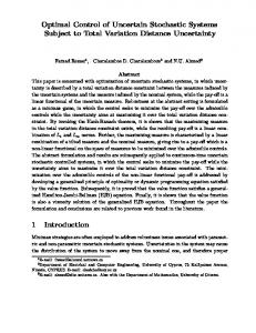
This example is an optical cavity coupled to three input channels v , w, u and three output channels x , y , z as shown in

(31)

Figure 2. An optical cavity A1 (t ), A2 (t ), A3 (t ) represent the input fields of channels v , w, u , respectively and

Using Lemma 4, this statement is equivalent to:

P  0 I 

B1 (t ), B2 (t ), B3 (t ) represent the output fields of channels (32)

x , y , z , respectively. Dynamics of this optical cavity are described by the * annihilation, a , and creation, a , operators.

Therefore, existence of such a self-adjoint, positive–definite matrix, P , which satisfies the inequality (32), is sufficient for stability of A and the proof is completed for A. Also, one may rewrite (32) as:

 A nT P  PA n  P 

(34)

■

(A n  A )† P  P (A n  A )

 A n † P  PA n   2 I  P 

0

 min  Subject to:   T  P P 0,  0 and  A nT P  PA n P I    P I 0 0  0   I   I 

Proof: By Lyapunov stability theory, A is stable if there exists a self-adjoint, positive–definite matrix, P , such that

A †P  PA  0 .

I

Existence of such P is equivalent to feasibility of the following

B. The following linear matrix inequality is feasible and



P

 I   0 0 1   2 

P  I  2      I I   0 

0  0

(33)

Again using Lemma 4, this is equivalent to:

6

where 

w

x

The perturbation parts are defined to be:

y

v

a

k1

S  I     k1 ( 1   1) 0  k1        L   c ,  c  X  (t )  0 0  X  (t )   0 0     

k2

k3 u

z

 k1  k2  k3 is the nominal attenuation ratio.

(38)

H   a * a

Figure 2. An optical cavity, which is coupled to three input and three output channels.

Let

A(t ) B(t ) X (t )

us

define

the

 A1 (t ), A2 (t ), A3 (t )  , T  B1 (t ), B2 (t ), B3 (t )  ,  a (t )  . T

the and

input

field

output

field

state

vector

the

Also, the nominal parameters are:

Sn  I  k1  Ln   Cn  , Cn   X n (t )   k2   k3  Hn  0 

The original uncertain plant parameters are:

S  I3  k1     L  [C  , C  ] X (t )   k2   k3  H   a*a

0  0  X (t )  0 

(36)

  ( I , L, H  Im( Ln † L)) Gn  ( I , Ln , 0)

and

 

   2 An    0  

.

     2  2i d X   0     k1     0 

   X (t )dt     2i  2  0

 k2

 k3

0

0

0

0

 k1  

 k2

 k1     k2   k3  d B (t )    0  0   0 

  2  k 1  2  k 1   k 1  2i  A    0  

0    d A(t )  k3 

  0    0   X (t )dt  d A(t ) k1    k2   k3  0

 0      2

(41)

which is stable since   0 . Also, the state matrix of the uncertain subsystem is:

The state-space realization of this LSQS is obtained as: 

(40)

where the state matrix of the nominal subsystem is:

of k1 , which plays a critical role in the plant dynamics. Prior knowledge about these uncertain parameters is taken into

 

(39)

Using the decomposition algorithm proposed in Theorem 1, the cavity plant is broken down into the following two subsystems:

where  is the “detuning” parameter and is related to the difference between the external field frequency and the cavitymode frequency. Also,  denotes the uncertainty in the value

consideration as

0   0  X n (t )  0 

   (42  k 1   k 12   k 1  2i   ) 2 

Matrices A  and  A can be computed as: (37)

7

0

The proposed systematic procedure for robustness analysis is summarized as follows:

k  k 2 k  0 1 1 1  A   2   0 k  k   k 1 1 1      0   2  2i   A      0   2i     2 

(43)

1.

Determine the uncertain parameters and their bounds.

2.

Use the decomposition presented in Theorem 1 in order to extract the nominal system from the uncertain system in the optical realization.

3.

Use the extended decomposition presented in Theorem 1 in order to decompose the system state matrix to the nominal and the additive normbounded uncertain parts.

4.

Use Theorem 2 or Theorem 3 in order to check robust stability of the system in the presence of uncertainties.

It is obvious that:

A  A n  A

(44)

As it was expected. Thus, we have evaluated the additive perturbation to the state matrix.

In complex networks, availability of an algorithmic and systematic approach for decomposition of the uncertain parts is of critical importance since in such networks handcrafted calculations may not be feasible. Adopting the LMI approach for solving the corresponding minimization problem and the norm-bounded assumption on additive perturbation state matrix may lead to conservative designs that guarantee the robust stability. However, this issue is outweighed by the practical value of the proposed method, when it comes to complex networks. Achieving less-conservative designs will be the focus of future research.

In order to check the robust stability, the total attenuation rate is chosen to be   k1  k2  k3  3 . Using the first approach, by numerical simulations,





inf  i  I A n  1.5 

. Thus, by Theorem 2, the sufficient condition for robust stability is:

  1.5

(45)

This upper bound can be rewritten based on the upper bounds on the uncertain parameters. Then, in order to achieve robust stability in the sense of Definition 2, the following inequality must hold:

A   

2 4

APPENDIX: PROOFS The following lemmas will be used in the proof:

 4  1.5 2

Lemma 3. for arbitrary matrices A, B 

(46)

A †B  B †A  A †A  B †B

0  1.4962 P   1.4962   0

Lemma 4 [31, 32]. (Schur compliment): For an arbitrary square matrix, which is partitioned to non-singular block-

(47)

square sub-matrices,

In order to guarantee the robust stability, the following bound condition must hold regarding (28) and the perturbation state matrix in (16):

 1.49

which is the same as the previous result.

(49) ■

  0.4445



, the following

statement holds:

Using Theorem 3, the following solutions are obtained for the minimization problem (28):

 1

n

A A   11  A21

A12   , the following A22 

statements are equivalent: I. A0 II.

(48)

A22  0 and A11  A12 A22 1 A21  0 REFERENCES

■

This example shows how the proposed theorems provide us with a systematic procedure to decompose the uncertain and certain parts of a linear quantum network in order to facilitate investigation of network’s robust stability.

[1]

[2]

VI. CONCLUSION In this paper, a robust stability analysis algorithm was proposed for general uncertain LSQS in the optical realization.

[3]

8

P. Azodi, A. Khayatian, P. Setoodeh, and M. H. Asemani, "Uncertainty Decomposition of Uncertain Linear Stochastic Quantum Networks," submitted to Systems and Control Letters. J. Gough and M. R. James, "The series product and its application to quantum feedforward and feedback networks," IEEE Transactions on Automatic Control, vol. 54, no. 11, pp. 2530-2544, 2009. M. R. James, H. Nurdin, and I. R. Petersen, "Control of linear quantum stochastic systems," Automatic

[4]

[5]

[6]

[7]

[8]

[9]

[10]

[11]

[12]

[13]

[14] [15]

[16]

[17]

[18]

[19]

[20]

Control, IEEE Transactions on, vol. 53, no. 8, pp. 1787-1803, 2008. I. R. Petersen, "Quantum linear systems theory," in Proceedings of the 19th International Symposium on Mathematical Theory of Networks and Systems, 2010. V. Belavkin, "Measurement, filtering and control in quantum open dynamical systems," Reports on Mathematical Physics, vol. 43, no. 3, pp. A405-A425, 1999. V. Belavkin, "Towards the theory of control in observable quantum systems," arXiv preprint quantph/0408003, 2004. V. P. Belavkin, "Quantum stochastic calculus and quantum nonlinear filtering," Journal of Multivariate analysis, vol. 42, no. 2, pp. 171-201, 1992. H. Mabuchi and N. Khaneja, "Principles and applications of control in quantum systems," International Journal of Robust and Nonlinear Control, vol. 15, no. 15, pp. 647-667, 2005. H. M. Wiseman and G. J. Milburn, Quantum measurement and control. Cambridge University Press, 2009. H. Wiseman, "Quantum theory of continuous feedback," Physical Review A, vol. 49, no. 3, p. 2133, 1994. H. Wiseman and G. Milburn, "Quantum theory of optical feedback via homodyne detection," Physical Review Letters, vol. 70, no. 5, p. 548, 1993. C. D’Helon and M. James, "Stability, gain, and robustness in quantum feedback networks," Physical Review A, vol. 73, no. 5, p. 053803, 2006. A. I. Maalouf and I. R. Petersen, "Bounded real properties for a class of annihilation-operator linear quantum systems," Automatic Control, IEEE Transactions on, vol. 56, no. 4, pp. 786-801, 2011. D. d'Alessandro, Introduction to quantum control and dynamics. CRC press, 2007. L. Bouten, R. Van Handel, and M. R. James, "An introduction to quantum filtering," SIAM Journal on Control and Optimization, vol. 46, no. 6, pp. 21992241, 2007. D. Dong and I. R. Petersen, "Quantum control theory and applications: a survey," Control Theory & Applications, IET, vol. 4, no. 12, pp. 2651-2671, 2010. I. R. Petersen, V. Ugrinovskii, and M. R. James, "Robust stability of uncertain linear quantum systems," Philosophical Transactions of the Royal Society of London A: Mathematical, Physical and Engineering Sciences, vol. 370, no. 1979, pp. 53545363, 2012. D. Dong and I. R. Petersen, "Sliding mode control of quantum systems," New Journal of Physics, vol. 11, no. 10, p. 105033, 2009. D. Dong and I. R. Petersen, "Sliding mode control of two-level quantum systems," Automatica, vol. 48, no. 5, pp. 725-735, 2012. J. Gough and M. R. James, "The series product and its application to quantum feedforward and feedback

[21]

[22]

[23] [24] [25]

[26]

[27]

[28]

[29] [30] [31]

[32]

[33]

9

networks," Automatic Control, IEEE Transactions on, vol. 54, no. 11, pp. 2530-2544, 2009. J. E. Gough, M. James, and H. Nurdin, "Squeezing components in linear quantum feedback networks," Physical Review A, vol. 81, no. 2, p. 023804, 2010. A. I. Maalouf and I. R. Petersen, "Coherent H∞ control for a class of linear complex quantum systems," in American Control Conference, 2009. ACC'09., 2009, pp. 1472-1479: IEEE. J. J. Sakurai and J. Napolitano, Modern quantum mechanics. Addison-Wesley, 2011. R. Shankar, Principles of quantum mechanics. Springer Science & Business Media, 2012. C. Gardiner and P. Zoller, Quantum noise: a handbook of Markovian and non-Markovian quantum stochastic methods with applications to quantum optics. Springer Science & Business Media, 2004. H. Mabuchi, "Coherent-feedback quantum control with a dynamic compensator," Physical Review A, vol. 78, no. 3, p. 032323, 2008. C. Gardiner, "Driving a quantum system with the output field from another driven quantum system," Physical review letters, vol. 70, no. 15, p. 2269, 1993. R. L. Hudson and K. R. Parthasarathy, "Quantum Ito's formula and stochastic evolutions," Communications in Mathematical Physics, vol. 93, no. 3, pp. 301-323, 1984. K. Zhou and J. C. Doyle, Essentials of robust control. Prentice hall Upper Saddle River, NJ, 1998. K. Zhou, J. C. Doyle, and K. Glover, Robust and optimal control. Prentice hall New Jersey, 1996. C. Scherer and S. Weiland, "Linear matrix inequalities in control," Lecture Notes, Dutch Institute for Systems and Control, Delft, The Netherlands, vol. 3, 2000. S. P. Boyd, L. El Ghaoui, E. Feron, and V. Balakrishnan, Linear matrix inequalities in system and control theory. SIAM, 1994. H.-A. Bachor and T. C. Ralph, "A Guide to Experiments in Quantum Optics, 2nd," A Guide to Experiments in Quantum Optics, 2nd, Revised and Enlarged Edition, by Hans-A. Bachor, Timothy C. Ralph, pp. 434. ISBN 3-527-40393-0. Wiley-VCH, March 2004., p. 434, 2004.