Dec 12, 1998 - Traditional compiler optimizations statically analyze and rewrite programs with the goal of .... ROE is primarily a framework for building.
ROE: Runtime Optimization Environment Marat Boshernitsan, Alyosha Efros, and David Oppenheimer {maratb,efros,davidopp}@cs.berkeley.edu December 12, 1998 Abstract Traditional compilers rely on static information about programs to perform optimizations. While such optimizations are effective, the programs can often be further optimized if frequent paths through the code and/or common data values are known to the compiler. Such information can be exploited by profile-based optimizers, but such optimizers can be foiled given sufficiently dynamic behavior of programs. In this paper we propose a software/hardware architecture for continuous profiling and dynamic reoptimization of programs. We discuss the advantages and tradeoffs of such an architecture and describe a prototype implementation. While our implementation should be considered work-in-progress, the preliminary results presented here are encouraging, indicating that dynamic reoptimization techniques may indeed be beneficial and should be explored further.
1
Introduction
Traditional compiler optimizations statically analyze and rewrite programs with the goal of improving performance for all possible executions of the program. These optimizations are therefore limited to those that will not harm the efficiency of the program for any particular input. Examples of such optimizations include dead-code elimination, which removes operations whose results are never used, common subexpression elimination, which allows common subexpressions to be reused among multiple computations rather than being computed once per such computation, and loop-invariant code motion, which moves out of a loop code that computes the same value on each iteration. Profile-based optimization removes this “do-no-harm” limitation by collecting profile information about a program during one or more runs of the program and using the profile information to guide optimizations that may penalize program efficiency in the uncommon case while improving program performance in the common case. Such optimizations are not possible without profile information because without such information it is difficult to distinguish the common from the uncommon cases.1 Examples of profile-based optimizations include selective procedure inlining, in which profile information is used to ensure that procedures are inlined only at sites from which they are called often, and code layout that colocates code from frequently-executed paths while moving rarely used code (e.g. exception handlers) to distant locations where it will not interfere with the frequently-executed code. Unfortunately profile-based optimizations suffer from two drawbacks. First, the statistics these optimizations use come from executing an unoptimized program on one or more “training” inputs. These training inputs may not match the user’s common inputs to the program, in which case the optimizations may provide no benefit or may actual decrease program performance. This problem is not merely hypothetical; some programs, such as interpreters, by their very nature exhibit different profiles across multiple executions. Second, the behavior of a program may change over a single run: the common path through a particular section of code, for example, may shift from a strong tendency towards one pattern to a strong tendency towards another, suggesting a need to reoptimize that section of code for the new common path. One solution to these problems is runtime optimization. Runtime optimization continuously profiles control-flow paths, and possibly data values, during program execution and continuously reoptimizes the program based on these observed frequently-executed control-flow paths (traces) and possibly data values. Performing these optimizations at runtime addresses the difficulty of selecting a good “training” input, while performing these optimization continuously addresses the possibility that program behavior may change during the execution of a single program. Runtime optimization is similar to profile-based optimization in that it improves program performance in the common case while possibly decreasing performance for uncommon control flow or data values.
1. This information can sometimes be predicted statically, as described in [19].
1
Even fairly simple runtime analyses can yield substantial optimization opportunities. For example, consider the following code adapted from an example in [6]: foo:
L1:
L2:
addui $sp, $sp, -4 sw $s1, 0($sp) sw $ra, 4($sp) addui $s1, $r2, 1 add $r2, $r3, $r4 bne $s1, L2 jal bar add $r5, $r1, $r2 sw $r5, 40($gp) lw $s1, 0($sp) lw $ra, 4($sp) addui $sp, $sp, 4 jr $ra
# make room on stack for two values # store callee-saved register on stack # store return address on stack # compute value to be used in block L1 # procedure call
# # # #
reload saved value of callee-saved reload saved return address pop stack frame return from procedure foo
If we know that the common path through procedure foo goes directly from the first block of the procedure to block L2, skipping block L1, we can remove a great deal of code. First, we have changed a non-leaf procedure into a leaf procedure by removing the procedure call to bar. This means we no longer need to save and restore the return address in lines 3 and 11 above. Second, we notice that the unoptimized procedure uses callee-saved register r1 because the value of r1 is used across the procedure call to bar. The common path does not make the call to bar, so it is safe to allocate that value to a temporary register, since no intervening code outside of foo can change it. This reallocation means we no longer use r1 inside of foo, and therefore we do not need to save and restore it in lines 2 and 10 above. Because we have now eliminated all use of the stack frame, we can also eliminate lines 1 and 12, which serve only to create and destroy the stack frame. Finally, we notice that the value computed in line 5 is only used in block L1, so it is dead code along the path that skips block L1. Having performed the above analysis, we can rewrite foo as foo’. foo’ consists of the optimized code for the path foo>L2, along with a check to see whether the path foo>L2 is actually taken for a particular invocation of foo. If the path foo>L1>L2 is actually taken, this check code branches into a “fixup” block of code that performs the operations necessary to develop the machine state that would normally be seen at the end of block L1, prior to jumping to block L2 in the original unoptimized program. This concept of “fixup code” is central to the runtime optimizations we will describe in this paper, as it allows the program to proceed correctly even in the case that the uncommon control-flow path is taken. In Section 6 we discuss alternative methods for detecting that such an uncommon path was taken. The optimized procedure foo appears below. We optimize by making a copy of procedure foo, called foo’, and optimizing that copy, while leaving the original unoptimized procedure intact. This allows us to branch out of the optimized procedure, through fixup code, back to the unoptimized procedure whenever we leave the trace. Without a copy of the unoptimized procedure available, we would continually jump back and forth between fixup code and the optimized trace, leading to unnecessary degradation of program performance in the uncommon case. foo’: addui $t1, $r2, 1 beq $t1, fixup jr $ra fixup:addui $sp, $sp, 8 sw $s1, 0($sp) sw $r1, 4($sp) add $r2,$r3,$r4 mov $t1, $s1
2
Note that in optimizing we reversed the sense of the branch that ends basic block foo. This is a general principle in how we lay out traces when we copy them from the unoptimized program prior to optimizing: we want the fallthrough of the branch to remain in the trace, and the branch-taken condition of the branch to exit to fixup code. This requires reversing the sense of the branch in the case where the original code fell through into the uncommon case (or conversely, branched to the next block of the common path). Though we will not provide a detailed example here, we note that programs can be specialized for common data values just as for common control-flow paths. This idea builds on the control-flow specialization we have already described: once a frequently-executed path is detected and optimized as above, the profiling mechanism starts observing the register values on entry to the trace. When the profiler notices that a trace is entered with one or more register values almost always the same, it may cause the creation of a copy of the control-flow-optimized trace and specialize it for those register values. This is similar to constant propagation but is performed at runtime. We describe this optimization in more detail in Section 6.1. .This paper describes ROE, the Runtime Optimization Environment. ROE is primarily a framework for building optimizations of the type we have described earlier in this section. It provides a profiling mechanism that monitors all branches taken by a program, an optimizer that builds a control flow graph of the program on the fly using this information, an interface between the profiler and optimizer that allows the profiler to ask the optimizer to optimize a trace the profiler has observed to be frequency executed, optimizer routines that select and copy a trace while creating proper fixup code to rejoin unoptimized code in the case of a branch out of the trace, dataflow analysis to support removal of dead code (e.g. the add in block foo above), and a mechanism to inject the optimized trace into the (simulated) processor and to fix up the unoptimized program code to branch into the trace. We begin in Section 2 with a high-level description of the ROE hardware/software architecture. Section 3 describes the profiling and optimization processes in more detail, and Section 4 describes how we evaluated the various components of the ROE system. Section 4 discusses the status of current prototype implementation In Section 6 we speculate on possible future work, in Section 7 we describe several of the difficulties we encountered in the course of this project, in Section 8 we examine related work, and in Section 9 we conclude.
2
Hardware/software architecture
Runtime optimization can be implemented in many ways, ranging from those in which the runtime profiling and optimization are performing completely in hardware, to those in which these functions are performed purely in software. For the purpose of this project we describe a design that falls close to the purely hardware end of this spectrum. We note, however, that this distinction in largely artificial: what we describe in the remainder of this section as separate hardware units could be implemented as communicating processes or threads on a commodity microprocessor, assuming some cooperation from the operating system.
2.1
Hardware structure
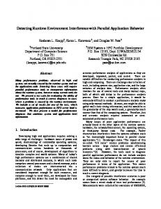
Our proposal for a hardware/software implementation of ROE, called ROE-1, is illustrated in Figure 1. It consists of three logical units: a main processor with its associated caches and memory, a profiler, and an optimizer. ROE-1 is designed to optimize a single process at a time. We now turn to a discussion of these hardware units and their interactions. 2.1.1 The profiler The profiler is a small piece of specialized hardware that receives the source and target virtual addresses of every branch taken by the CPU, along with the process ID of the executing process and the type of branch (conditional direct, conditional indirect, unconditional direct, or unconditional indirect). If the process ID of the executing process matches the process ID that the profiler is monitoring, the profiler updates its internal table of branch counts to reflect the taken and not-taken branch paths. It also increments a counter associated with the target pc, which represents a count of the number of times the basic block that begins at that pc has been executed. If the incremented basic block
3
Threshold
CPU core
L1$
PROFILER PID
flush
add/hint
iCache flush
OPT
access
L2$ MEM
REGS
MEM
read program instr / write new instr
Memory mapped registers
Figure 1: High-level hardware/software architecture of ROE
count reaches a threshold value, the profiler invokes the optimizer with that pc, as a suggestion to the optimizer that it could be profitable to build and optimize a trace around the basic block that begins with that pc. Additionally, each time the profiler sees a new edge, it notifies the optimizer, which updates its data structure representing the dynamic control-flow graph it builds as the program runs. (See Section 3.2) The profiler must be able to accept one branch address per CPU cycle (assuming a CPU that can commit one branch instruction per cycle). While this may seem at first infeasible because each branch requires an update to a fairly large table, a pipelined implementation of the profiler suggests that such hardware is realizable. As suggested in [20], updates to the profiler’s data structure can be pipelined: the “repeat rate” of updates must be one every few CPU cycles, but the actual latency of updates can be much longer because at worst this latency results in a slight delay between when a basic block threshold is actually reached and when the profiler notices that it has been reached. Moreover, because the data we collect need not be precise, it is acceptable for the profiler to ignore branches that it is too busy to process. Though in that case the statistics gathered by the profiler will be less precise than they would be if every branch were recorded, we are interested in gross behavior of the program that is not sensitive to missing a small percentage of all the branches executed. 2.1.2 The optimizer The optimizer is the core hardware structure in ROE-1. It contains a general-purpose memory (in contrast to the very regular hardware table used by the profiler) for use as internal scratch space, memory that can be used to communicate with the CPU (e.g. that is mapped into the CPU’s address space and that can be read and written by the CPU’s operating system), and the optimization program itself. The optimizer is notified by the profiler of every newly-discovered edge in the program. The optimizer uses this information to build a dynamic control-flow graph in the form of a data structure that maps every pc in the program to the basic block containing it; this data is stored in the 4
optimizer’s scratch memory space. The unoptimized program is initially represented as a single basic block; when a branch is detected, the source block is split at the branch and the target block is split at the branch target. A basic block is represented by pointers to the first and last instruction in that basic block in the original program. Controlflow edges are purely stored in the profiler; the optimizer queries the profiler for these edges when it later needs them to perform optimization. As mentioned in the previous section, the profiler notifies the optimizer with a “hint” pc around which the optimizer should consider building a trace. Upon receiving this signal, the optimizer selects a trace by starting with the basic block containing the “hint” pc and copying basic blocks from the original program, growing the trace forwards and backwards from that point; this process is described in detail in Section 3.3. These trace cells are copied into optimizer memory that is mapped into the address space of the CPU; as trace cells are copied from the original program, they are laid out linearly in memory; hence we call this process trace copying. At the same time, trace cells for later insertion of fixup code (fixup cells) are created. The trace is now ready for optimization, which we describe in detail in Section 3.4. After performing optimizations and linearization (assigning consecutive addresses to instructions) on the trace stored in optimizer memory, the optimizer sets a flag that can be read by the operating system (denoted REG in Figure 1, to indicate that this may be implemented as a register mapped into the CPU’s memory space); this flag indicates that a trace has been optimized and is ready for injection. The operating system handler that incorporates the optimized trace is described in the next section. At this point we note that ROE-1’s use of optimizer hardware distinct from the CPU hardware means that building the dynamic CFG and performing optimization can occur in parallel with the normal operation of the main CPU, therefore not affecting overall system performance. We do assume that the optimizer halts the CPU while it is injecting optimized code, though injection could in theory be overlapped with the main CPU running a process other than the one being optimized. The hardware requirements for the optimizer are different in several respects from those of the profiler. First, the optimizer builds a dynamic control-flow graph and also performs linearization and optimization, so it is more akin to a general-purpose CPU than to the branch-prediction hardware that the optimizer resembles. Second, the frequency of received external events (newly-discovered edges from the profiler) starts out equal to that for the profiler (which receives notification of every branch taken by the CPU) but decreases as the program’s edges are discovered. This further argues for a general-purpose hardware structure, so that resources can be dedicated to processing new-edge events near the beginning of a program’s run and can be rededicated to performing optimizations later on. We have until now ignored the possibility of the profiler’s edge table or optimizer’s CFG structure becoming full. A ROE system implemented in hardware must deal with this situation; a software implementation could rely on virtual memory paging of the relevant data structures when they grow large, though eventually this will hurt performance more than the optimizations help and will therefore become a detriment to the system. Therefore either type of ROE implementation needs to notice when these data structures reach a maximum allowed size (“hardware table full” in the case of profiler in hardware, and “scratch memory full” in the case of the optimizer in hardware) and either stop recording new information or flush the current data. The first option is unattractive because it means the program can no longer be optimized: not only will new optimization opportunities be lost, but more importantly a shift in program behavior that favors a previously infrequent path over a previously frequent (and optimized-for) path could result in many executions of a trace that result in exit through fixup code, thus hurting program performance over an unoptimized version of the program. We therefore use the second approach: when the profiler data structure becomes full, the profiler flushes itself and sends a “flush” signal to the optimizer, which flushes the CFG it is building and starts over again. Because each new edge recorded in the profiler’s edge table can result in at most two new basic blocks in the optimizer CFG (one basic block is split at the branch source, and another basic block is split at the branch target), we can size the optimizer scratch memory so that it will never become full before the profiler becomes full and sends it a flush signal. 2.1.3 The CPU ROE-1 assumes a modern commodity microprocessor that has been modified to signal the source and target address of each branch encountered by an executing program; as described above, this information is used by the profiler. We 5
assume the optimized trace is stored in the optimizer in memory that is mapped into the address space of the CPU; this can be accomplished by connecting the optimizer to the memory bus side of the memory bus controller. When the optimizer has prepared an optimized trace, it sets a flag (either in a register that can be read by the CPU or in its memory mapped into the address space of the CPU). The operating system checks this flag before each context switch into the process that is being optimized. If the flag is set, the CPU enters an operating system handler that extends the indicated process’s text segment (by updating the TLB and page table) by the amount of extra code represented by the trace and its associated fixup cells, reads the trace out of the optimizer memory, translates the virtual addresses in the trace to physical addresses, and inserts the code into the newly-extended text segment via the L2 cache. We assume the L2 cache replacement policy handles writebacks to memory. The operating system handler also reads a list of instructions in the old program that need to be patched to jump to the optimized trace, and patches these instructions similarly (translate virtual to physical address, update L2 cache). Finally, the L1 instruction cache, or just the lines in that cache that represent data that has been modified, are flushed. The operating system then clears the flag in the optimizer and returns to user code.
2.2
Operating system involvement and multiprogramming issues
We have already mentioned one complication arising from the use of a “commodity” microprocessor and operating system, namely the need to translate the virtual addresses used by the profiler and optimizer into physical addresses used by the caches and main memory. Multiprogramming and shared libraries further increase the level of operating system support required. ROE-1 is designed to optimize one program at a time. This decision was made primarily to limit the extra hardware and/or software required to handle multiprogramming. In ROE-1 a privileged user of the main CPU informs the operating system of the process ID (PID) of the process to optimize. The operating system writes this value into a register or memory-mapped location in the optimizer, and that information is then sent to the profiler. (In a slightly different design the CPU could write this information directly to the profiler; however, general communication between the CPU and the profiler is not permitted in ROE-1.) The profiler then matches this PID with subsequent PID’s tied to virtual addresses of branch sources and targets sent from the main CPU; only when the PID’s match is a branch recorded in the edge table and associated tables. This PID is also compared against when the operating system is performing a context switch; only context switches to this process trigger a check of the optimizer flag that indicates whether a new trace has been prepared for injection into that process. To handle simultaneous optimization of multiple processes, the profiler table and optimizer CFG data structure could either be replicated per process being optimized or data could be tagged with the PID of the process with which it is associated. Alternatively, a single structure could be used, and its contents could be swapped by the operating system when a context switch is made to a new process that is being optimized. Even when optimizing a single process, ROE-1 must handle the possibility of shared text segments, such as those used by multiple processes dynamically linked with the same shared library. In this case the operating system could employ some sort of “copy-on-write” mechanism to deal with optimization of shared libraries. In particular, the manner in which we patch old code to jump into the optimized trace will affect all sharers of a shared library; but in reality we only want the process that is being optimized to see the new branches into optimized code -- for the other processes, the trace may not represent a frequent control-flow path, and as a result is unlikely to help (and indeed may hinder) program performance. Therefore either we will not optimize shared text segments, or when a shared text segment is optimized, a copy of the old code (or at least those pages of the old code that are being modified to jump into a trace) must be made before being modified; these pages are associated with the optimized program, and the unmodified old code pages remain associated with all the other sharers. Whether the traces appended to the text segment are shared is irrelevant, since only the process that sees the patched old program code will ever jump into a trace. In Section 6.3 we discuss alternative hardware implementations of vectoring to fixup code; one solution we propose that could avoid the need to do copy-on-write would be for hardware to compare the PID of the process that reaches the beginning of a block that has been used as the head of a trace against the PID(s) the trace was optimized for, automatically setting the “next pc” to the appropriate fixup code for that block if they match.
6
ROE-1 could potentially be used to optimize operating system code as well as user code. The goal in this case would be to identify frequent paths through operating system code, either on a per-user-process or global basis. The same difficulty with shared code arises here, though there are extra complications in this case because the “process” that is being patched is also doing the patching. We do not consider these issues further, as this paper focuses on optimization of user-level code. Because our simulation environment (SimpleScalar) simulates only a single user-level process, we did not implement the copy-on-write mechanism for modified shared code, features needed to support multiprogramming, or any operating system code optimizations.
2.3
Simulation environment
We used the SimpleScalar simulator [21] as the basis of our processor simulation environment. We simulated an outof-order processor containing four integer ALU’s, four floating point ALU’s, one integer multiply/divide unit, and one floating point multiply/divide unit. The ISA for the simulated processor is based on the MIPS IV; code was generated using a version of gcc distributed with the simulator and that targets the SimpleScalar architecture. The simulated processor fetches, decodes, and issues up to four instructions per cycle. It also performs branch prediction (using a bimodal predictor with 2048 BTB entries) and speculative execution; the branch misprediction latency is three cycles. The simulated processor has separate L1 instruction and data caches; each can be accessed in one cycle and is 8 KB in size, direct-mapped, and write-back, with 256 sets, 32-byte blocks, and LRU replacement. The simulated processor also has a merged L2 cache, with a 6 cycle access latency. The L2 cache is four-way setassociative, write-back, and 256KB in size, with 1024 sets, 64-byte blocks, and LRU replacement. The main memory access latency is 18 cycles for the first 8 bytes, and 2 cycles for subsequent 8-byte units. The TLB miss latency is 30 cycles; we simulate a 64-entry, 4-way set associative ITLB with 4K pages, and a 128-entry, 4-way set associative DTLB with 4K pages. Both TLB’s use LRU replacement.
3
The optimization process
In this section we examine several details of the profiler and optimizer in more detail.
3.1
Gathering statistics and triggering the optimizer
As previously mentioned, the profiler is a piece of fast, specialized hardware connected between the CPU and the optimizer. Conceptually, the profiler acts as an information filter that gathers statistics about program execution, tabulates those statistics, and when queried by the optimizer feeds them into the optimizer in a much more compact form. The desired functionality of the profiler can the summarized as follows: • Program branches must be detected and recorded (this recording must be fast) • Information about new control-flow edges and newly-detected hot basic blocks must be relayed to the optimizer. • The following types of queries from the optimizer must be supported (response time should be reasonable but is not constrained by the CPU speed): - Given an address of a branch (or a branch target) that is the end (the beginning) of a basic block, return the number of times the branch has been executed. - Given an address of a branch (a branch target), return all control flow edges that have this address as the source (destination) together with the count of the number of times each edge was taken. These requirements dictate the need to support fast queries on branch addresses and branch target addresses, as well as the need to keep lists of edges going from (to) a particular address. Conceptually, this means a data structure with all control edges plus two lookup tables indexed by branch (branch target) address and containing a list of pointers into the edge structure. Since the data structure is finite, a mechanism is needed for handling the situation when it fills up.
7
Table 1: Direct Branch Address (DBA) Table Tag
Branch Addr
Branch Count
Target Addr
Edge Count
Link1
Link2
Table 2: Indirect Branch Address (IBA) Table Tag
Branch Addr
Branch Count
Target1
Count1
Link1
Target2
Count2
Link2
.. .
Table 3: Branch Target Address (BTA) Table Tag
Branch Target Count
Link Head
Link Tail
Figure 2: Hardware structure of profiler tables
One way to implement the profiler in hardware is to use three hash tables (implemented in hardware as set associative caches) shown in Figure 2 and some simple logic to manipulate and update them. The DBA (direct branch address) and IBA (indirect branch address) tables store the forward mapping from Branch Addresses to Branch Target Addresses for all edges. For the DBA table, we use the fact that for direct branches, there are at most two ways to proceed: take the branch or fall through. The fall-through address is easy to calculate (branch address plus size of instruction), so we only need to store the branch-taken address. The same idea applies to counts: total count minus the count on one edge will give the count on the other edge so we don’t need to store it. We do, however, need to store two link pointers that are used to link up edges that go into the same branch target addresses. Indirect branches are different, however, because we don’t know the number of targets for such a branch. So, for the IBA table, we only record some fixed number of targets (say, 10), discarding all the rest. In all other respects, the IBA table has the same structure as the DBA table. The BTA (branch target address) table provides the reverse mapping by way of linked lists through the forward mapping structure. The head link points to the branch address that can jump to this target address, which in turn points to the next one in its link field and so on. The tail of this list also has a direct link from the BTA table to permit constant-time insertions. Every time the CPU executes a branch instruction, the profiler is told the type of branch, the current PC (PC), and the target PC (NPC). PC is used to index into either the DBA (for direct branches) or the IBA table (for indirect branches). If no entries exist, a new entry is added, and the corresponding entry in the BTA table is also created. If an entry exists for this branch in DBA or IBA tables, we try to match the NPC to the ones stored in the entry (in parallel). If we are successful, only counts need to be updated. If not, the NPC is recorded, and appropriate links are added in the BTA table.
8
0x1234: bne r1, r2, 0x5678
0x1234: bne r1, r2, 0x5678 a 0x1238: ...
b
c 0x5678: ... Figure 3: Refinement of the DCFG by splitting a basic block on a newly-encountered branch
The proposed hardware satisfies all 3 requirements above. The profiling is done mostly in parallel and thus is quite fast. Forward queries are also fast (constant time) while reverse queries are slower (due to linked lists) but still sufficient for the purpose of servicing queries from the optimizer.
3.2
Dynamic Control Flow Graph Construction
When a flow edge (corresponding to a control flow transfer via a conditional branch or an unconditional jump) is encountered by the profiler for the first time, the optimizer is notified to update its notion of the program’s control flow graph. We call this flow graph that the optimizer continuously builds on the fly the Dynamic Control Flow Graph (DCFG) to distinguish it from a static CFG of the type constructed by a static compiler during compilation. The important feature of the DCFG is that it only includes those static CFG edges that have actually been traversed thus far during the given execution of the program and that are therefore relevant for selecting a hot path (trace) through a section of the program. When a program starts executing, the optimizer considers the entire program to consist of a single basic block. Each time a control transfer instruction is executed, the basic block corresponding to the instruction’s PC as well as the basic block corresponding to the target PC are split, resulting in a refinement of the DCFG. Figure 3 demonstrates the actions taken by the optimizer when a conditional control transfer instruction is encountered by the profiler for the first time. First, the basic block to which instruction belongs is located and split at a point immediately following the instruction, resulting in edge a. Second, the basic block containing the target of control transfer is split immediately before the target address, resulting in edge b. (As mentioned above the profiler treats fall-through cases of conditional branch instructions as new flow graph edges, so the optimizer is informed of the two new flow edges, rather than one). Lastly, the so-called “fall-through” edge c is added preceding the basic block that is the target of the jump. It should be noted that the flow graph edges are not explicitly stored by the optimizer; rather, each time the optimizer needs to traverse the flow graph, it queries the profiler for the flow graph edges leading into/out of a basic block. This implementation is not as inefficient as it may seem, since the only time the optimizer traverses the flow graph is during the trace construction, at which point it also needs to obtain the up-to-date edge traversal counts from the profiler. A bit of extra logic is used to calculate counts for “fall-through” edges in the DCFG that do not correspond to any taken branch recorded by the profiler.
3.3
Selecting a trace
Upon receiving a hint from the profiler that a certain target PC has been executed a sufficient number of times to be considered the kernel of a trace (this number is a configurable parameter of the profiler), the optimizer fires and tries to select a trace starting at the target PC’s basic block. The algorithm for trace selection was adapted from [7]. 9
(a)
(b)
(c)
(d)
Figure 4: Four possible trace shapes after trace selection. Each box represents a basic block.
The optimizer starts by forming a trace consisting of a single hot basic block and then traverses the DCFG backward and forwards, forming a trace around the hot basic block. During the traversal, the optimizer considers all possible successors (predecessors during backward traversal) of the most recently-added basic block, trying to pick a candidate that is more likely to be on the hot path than is any other successor (predecessor). To pick a good candidate, the optimizer considers all edges leading out of (into) the current basic block, computing edge weight by normalizing edge counts so that they all edge weights add up to 100%. The optimizer then looks for an edge whose weight is above a certain threshold (this threshold is a configurable parameter of the optimizer). If such an edge is found, the optimizer attempts to add its destination (source) basic block to the trace. If no edge with weight above the threshold is found, the optimizer stops growing the trace in that direction. When attempting to add the selected basic block, the optimizer checks whether the block is already in the trace and, if so, also stops growing the trace in that direction. An additional condition for terminating trace growth is running into a section of code that has already been optimized. It should be noted that unlike previous trace selection algorithms, we do not require the trace to terminate at procedure boundaries. This results in longer traces with more optimization potential. Once a trace is selected, an additional traversal is used to verify that the selected trace is useful for optimization. While we allow the trace to have a single back-edge at the end that loops to the beginning of the trace, we disallow back-edges into the middle of the trace that may arise when instructions from both inner and outer loop are selected to be in the trace. Figure 4 shows four possible trace shapes after trace selection. Traces (a) and (b) are “good” and may be optimized, whereas traces (c) and (d) are “bad” and need to be discarded. After a trace passes the above “sanity check,” the instructions from the original program are copied into the trace’s basic blocks (trace cells). For the most part, copying instructions is straightforward. But because the trace is expected to be “linearized” in memory, copying of a control transfer instruction that may terminate the basic block is slightly more complicated and is performed in two steps. First, the trace copying algorithm “macro-expands” subroutine call instructions (JAL, JALR) into an instruction that updates the link register and the jump instruction itself, so that the jump instruction may be manipulated independently. In the second step, all possible control transfer instructions are considered and treated separately: • Direct unconditional jumps (including the ones that resulted from expansion of subroutine calls) are removed, as their target is presumed to follow in the trace anyway. • Indirect unconditional jumps are replaced with a sequence of instructions that compare the branch register with the value it is expected to have so that the thread of control stays in the trace. If the comparison fails, the thread of control leaves the trace through a special trace cell called a fixup block or fixup cell. The original indirect jump instruction is moved into this fixup code, ensuring that control will be transferred to the expected locations in unoptimized code. Since it is not known where fixup code will be laid out in memory, the branch instruction is marked for later address resolution. • A conditional branch whose “taken” target is not in the trace, is marked to be later resolved to point to the fixup trace cell. Additionally, an unconditional jump is placed into the fixup trace cell, so that after the fixup code, if any, is executed, control is correctly transferred back to the unoptimized program.
10
• A conditional branch whose “taken” target is in the trace is reversed (so that its fall-through case is in the trace) and is then treated like the other kind of conditional branch (see above). The control transfer instruction at the end of the trace needs to be treated slightly differently because its target may be the head of the trace (if the trace loops) rather then a subsequent trace cell. An example of a trace after selection may be found in Figure 5(a), and after copying and linearization in Figure 5(b).
3.4
Optimizing a trace
After selection and copying, the trace is ready to be optimized 1. Because we are operating at the instruction level where much high-level information about the original program has been lost, only a limited number of optimizations are feasible. The ones of particular importance are dead code elimination and procedure inlining [14]. Dead code elimination involves removing instructions whose results are not subsequently used, and procedure inlining eliminates the call overhead of frequently executed procedures by inlining procedure instruction at the call site. However, given that the optimizer selects traces across procedure boundaries, we get almost all of the benefits of procedure inlining, since dead code elimination will remove procedure call overhead 2. In order to discover dead code, the optimizer needs to perform dataflow analysis to compute the def-use and use-def chain for each instruction. The def-use chain links the instruction defining a value (register or memory location) with all instructions using that value before it is redefined. The use-def chains is the inverse, linking an instruction to all instructions defining its inputs. The def-use and use-def computation is a classic dataflow problem. Our implementation uses an iterative approach to this dataflow computation and, given that a trace may contain at most one loop, the number of iterations cannot exceed 2. Because the optimizer has no information about aliasing of memory locations, it conservatively assumes that almost all memory is aliased. In practice, this proves to be a severe restriction, since it prevents the optimizer from removing many loads and stores, especially the ones that correspond to register loads/stores in procedure prologues and epilogs. To alleviate this, we make an assumption that all memory operations with respect to the stack pointer register are not aliased, which allows us to compute precise dataflow information for those instructions3. Having performed this dataflow analysis, dead code elimination is straightforward. Our algorithm considers each instruction in the trace by marking it MAYBE_DEAD. In order to be considered dead, the instruction must satisfy the following conditions: • not be a control-transfer instruction, and • be marked MAYBE_DEAD or all of the instruction’s users must be dead. The last two conditions ensure that dependency cycles (when an instruction directly, or indirectly, depends on its own result via a trace back-edge) can be successfully broken. The last optimization step is the actual removal of dead code. Since the instructions are only dead inside the trace, we must be careful to produce fixup code that “undoes” the effect of our optimizations, should we accidentally exit from the trace. This fixup code is produced by copying a dead instruction into all possible trace exit points (fixup blocks) past the point at which the instruction was originally executed (before it was removed). If several instructions are to be placed in the same fixup block, we must be careful to preserve their relative ordering. If a fixup instruction depends on some inputs not available in its fixup block, the instructions producing those inputs must also be copied.
1. In a sense, copying and linearizing a trace is itself an optimization because it packs instructions from the trace together, improving the trace’s instruction cache locality. 2. This is not entirely true since we only get all the benefits of procedure inlining if the entire hot procedure ends up being in the trace. However, our experiments show that this happens quite often. 3. In a production implementation of ROE, we would like the compiler to provide some sort of guarantee that this is really the case.
11
findshapes (+0xcd8) pc0 = 0x47fc88 pc1 = 0x47fcb8 lw r11,52(r29) lw r2,-31212(r28) addiu r18,r18,1 addiu r11,r11,48 slt r2,r18,r2 sw r11,52(r29) bne r2,r0,0x47f070 (997)
findshapes (+0xc0) pc0 = 0x47f070 pc1 = 0x47f0a0 lw r10,52(r29) lw r6,-31384(r28) lui r8,0x1008 addu r8,r8,r10 lw r8,6428(r8) slt r2,r6,r8 bne r2,r0,0x47fc88
findshapes (+0xcd8) pc0 = 0x497ca0 (0x47fc88) pc1 = 0x497cd0 (0x47fcb8) lw r11,52(r29) lw r2,-31212(r28) addiu r18,r18,1 addiu r11,r11,48 slt r2,r18,r2 sw r11,52(r29) beq r2,r0,0x497d98
(2)
findshapes (+0xd10) pc0 = 0x47fcc0 pc1 = 0x47fd18 lw r31,92(r29) lw r30,88(r29) lw r23,84(r29) lw r22,80(r29) lw r21,76(r29) lw r20,72(r29) lw r19,68(r29) lw r18,64(r29) lw r17,60(r29) lw r16,56(r29) ... jr r31
pc0 = 0x497d98 (0x0) pc1 = 0x497d98 (0x0) j 0x47fcc0
findshapes (+0xc0) pc0 = 0x497cd8 (0x47f070) pc1 = 0x497d08 (0x47f0a0) lw r10,52(r29) lw r6,-31384(r28) lui r8,0x1008 addu r8,r8,r10 lw r8,6428(r8) slt r2,r6,r8 bne r2,r0,0x497d90
(1000) findshapes (+0xf8) pc0 = 0x47f0a8 pc1 = 0x47f0c8 lui r7,0x1008 addu r7,r7,r10 lw r7,6432(r7) slt r2,r6,r7 bne r2,r0,0x47fc88
pc0 = 0x497d90 (0x0) pc1 = 0x497d90 (0x0) j 0x47fc88
findshapes (+0xf8) pc0 = 0x497d10 (0x47f0a8) pc1 = 0x497d30 (0x47f0c8) lui r7,0x1008 addu r7,r7,r10 lw r7,6432(r7) slt r2,r6,r7 bne r2,r0,0x497d88
(999) findshapes (+0x120) pc0 = 0x47f0d0 pc1 = 0x47f110 lw r11,28(r29) lui r10,0x1005 addiu r10,r10,22064 addu r2,r11,r10 lw r2,0(r2) lw r20,20(r29) subu r2,r2,r8 addiu r4,r2,1 bgez r4,0x47f120 (595) findshapes (+0x170) pc0 = 0x47f120 pc1 = 0x47f140 lw r11,36(r29) lw r2,0(r11) subu r2,r2,r7 addiu r2,r2,1 bgez r2,0x47f150
pc0 = 0x497d88 (0x0) pc1 = 0x497d88 (0x0) j 0x47fc88
findshapes (+0x120) pc0 = 0x497d38 (0x47f0d0) pc1 = 0x497d70 (0x47f110) lw r11,28(r29) lui r10,0x1005 addiu r10,r10,22064 addu r2,r11,r10 lw r2,0(r2) lw r20,20(r29) subu r2,r2,r8 addiu r4,r2,1
(404)
findshapes (+0x168) pc0 = 0x47f118 pc1 = 0x47f118 addu r4,r0,r0
(a)
pc0 = 0x497d78 (0x0) pc1 = 0x497d80 (0x0) bgez r4,0x47f120 j 0x47f118
(b)
Figure 5: A trace after selection (a) and the same trace after copying and linearization (b). In trace (a), the dotted boxes represent the basic blocks that were not selected for the trace, and the numbers on the edges correspond to the number of times a given edge was executed. In trace (b), the dotted boxes represent the fixup code blocks.
12
4
Implementation status
We extended the base SimpleScalar simulator with modules corresponding to the profiler and optimizer, but we did not simulate the profiler or optimizer hardware themselves. Instead, we assume the optimizer runs in parallel with the main CPU, so there is no need to account for the time needed for optimization. We do simulate the cache effects of injecting optimized traces. The current implementation of the optimizer completely handles trace selection, copying, dead code elimination, linearization, and injection into the running program. Due to time constraints we did not test and evaluate dead code elimination optimization, but we hope to do so in near future. We do not perform flushing of the profiler or optimizer data structures. In addition, we have developed a graphical debugging framework based on the GraphViz Toolkit from AT&T. This toolkit can be used to generate graphs of the optimizer data structures; this framework was used to generate the graphs of the traces in Figure 5.
5
Evaluation
Due to time constraints we were unable to evaluate the performance impact of our code-reducing optimizations. We therefore evaluate the ROE framework with respect to selection of traces and the effect of reinjecting these traces into the executing program. In particular, we examine characteristics of the program (increase in text size resulting from the trace and fixup code, performance impact), static trace statistics, dynamic trace statistics, size of optimizer data structures, and the effect on cache miss rate resulting from injecting optimized code and from the execution of the traces themselves. Finally, we make some brief observations of the sensitivity of our metrics to edge threshold. We ran ROE on four modified SPECInt95 benchmarks. These benchmarks were "modified" in the sense that we ran them for only the first 70-100 million instructions due to time constraints 1. The benchmarks we ran were lisp, m88ksim, go, and gcc. We examined three ROE configurations: ROE disabled (unmodified out-of-order processor as described in Section 2.3; this is the baseline configuration to which we compare), ROE with a basic-block threshold of 10,000 and an edge threshold of 0.70, and ROE with a basic-block threshold of 10,000 and an edge threshold of 0.90. Here the "basic-block threshold" is the number of times a basic block is executed before the profiler sends a "hint" to the optimizer to optimize a trace forward and backwards starting from that block, and the "edge threshold" is the required branch frequency for a block to be added to the trace (i.e. the frequency that the edge is taken must be at least the edge threshold for the block at the other end of the edge to be added to the growing trace; otherwise growing the trace (forward or backward) is terminated.) Due to time constraints we did not thoroughly investigate the sensitivity of trace selection to basic block threshold; however, we did notice that (as expected) fewer traces were generated as the basic block threshold was increased.
5.1
Overall program characteristics
Figure 6a shows the number of traces that were created for each program while Figure 6b shows the total number of instructions that have been added to the programs (as a result of creating and injecting traces). We note that all four programs that we have tested are large; as a result, the effect of injecting additional program text has negligible effect on the overall program size. Figure 7 shows the percentage of overall time spent in, and instructions executed in, trace code. A high percentage means that the trace we have picked is indeed hot and worthwhile to optimize. We found a surprisingly high
1. This is admittedly a small fraction of the total number of dynamic instructions in these benchmarks.
13
Number of traces generated
Total instructions added
20
250 70% threshold 90% threshold
18
70% threshold 90% threshold
16
200
14
# instructions
# traces
12
10
8
150
100
6
4
50
2
0
1
2
3
4
0
1
2
3
SPEC programs
4
SPEC programs
(a)
(b)
Figure 6: Number of traces generated (a) and total instructions added (b) for SPEC benchmarks. [(1) = li, (2) = m88ksim, (3) = go, (4) = gcc]
Percentage of time/instructions spent in traces for 70% threshold
Percentage of time/instructions spent in traces for 90% threshold
70
70 % time spent in traces % instructions executed in traces
60
60
50
50
40
40
perentage
perentage
% time spent in traces % instructions executed in traces
30
30
20
20
10
10
0
1
2
3 SPEC programs
(a)
4
0
1
2
3
4
SPEC programs
(b)
Figure 7: Time spent in, and dynamic instructions executed in, traces for SPEC benchmarks. [(a) = 70% threshold, (b) = 90% threshold] [(1) = li, (2) = m88ksim, (3) = go, (4) = gcc] percentage of execution time spent in traces, especially considering that we only generated a handful of traces for each program. Figure 8 shows the percentage speedup (or slowdown) for each benchmark relative to the unoptimized program. The primary factor contributing to speedup is improved instruction-cache behavior resulting from compacting the instructions from a trace (i.e. removing intervening infrequently-executed instructions from the unoptimized
14
Miss−rate improvement over baseline for 70% threshold
Miss−rate improvement over baseline for 90% threshold
120
140 % L1 I−cache miss−rate relative to baseline % L2 cache miss−rate relative to baseline
% L1 I−cache miss−rate relative to baseline % L2 cache miss−rate relative to baseline 120
100
100
perentage
perentage
80
60
80
60
40 40
20
0
20
1
2
3
0
4
1
2
3
SPEC programs
(a)
(b) Speedup over baseline for 90% threshold 120
100
100
80
80
perentage
perentage
Speedup over baseline for 70% threshold 120
60
60
40
40
20
20
0
1
2
3 SPEC programs
(c)
4
SPEC programs
4
0
1
2
3
4
SPEC programs
(d)
Figure 8: Change in cache miss rate [(a) 70% threshold, (b) 90% threshold], and speedup [(c) 70% threshold, (d) 90% threshold], for SPEC benchmarks. [(1) = li, (2) = m88ksim, (3) = go, (4) = gcc] program). The primary factor contributing to slowdown is the extra jumps needed to get to the trace, and jumps associated with exit through fixup blocks of the trace. There is also some slowdown (and increase in instruction cache miss rate) associated with the fact that jumps to traces go far from (and therefore may conflict in the cache with) their source; in the unoptimized program, branch targets are usually near the branch source. Although we assume the optimizer runs in parallel with the CPU (and therefore does not impact program performance except by increasing cache miss rate when new instructions are injected into the L2 cache and L1 cache lines are flushed), we do include the time needed to inject new (optimized) code, since we propose to increase operating system context switch time by exactly the amount of time needed to load the trace when switching to a process that has new optimized code. This is 15
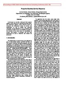
trace lengths for gcc
trace lengths for go
25
60 main trace code fixup code
main trace code fixup code 50
20
# of instructions
# of instructions
40 15
10
30
20
5 10
0
1
2
3
4
5 trace number
6
7
8
0
9
1
2
3
(a)
4
5
6 7 8 trace number
trace lengths for lisp
11
12
trace lengths for m88ksim 120 main trace code fixup code
main trace code fixup code
25
100
20
80 # of instructions
# of instructions
10
(b)
30
15
60
10
40
5
20
0
9
0
2
4
6
8
10 12 trace number
(c)
14
16
18
20
0
1
2 trace number
3
(d)
Figure 9: Static trace length distribution [(a) = gcc, (b) = go, (c) = li, (d) = m88ksim], 90% threshold calculated as 18 + 2*((N-8)/8) cycles, for a trace of N bytes, assuming the optimizer memory can be read with the same latency and bandwidth as main memory.
5.2
Trace statistics
We now turn to a discussion of static and dynamic trace characteristics. Figure 9(a-d) shows the sizes of each trace, divided into the contribution from trace code and fixup code. (Because we did not evaluate optimizations, fixup code is negligible.) Figure 10 shows the per-trace percentage of time spent in, and instructions executed in, each trace.
16
Percentage of time/instructions spent in traces for gcc
Percentage of time/instructions spent in traces for go
2.5
6 % time spent in traces % instructions executed in traces
% time spent in traces % instructions executed in traces 5
2
4
perentage
perentage
1.5
3
1 2
0.5 1
0
1
2
3
4
5 trace number
6
7
8
0
9
1
2
3
(a)
4
5
6 7 8 trace number
9
10
11
12
(b)
Percentage of time/instructions spent in traces for lisp
Percentage of time/instructions spent in traces for m88ksim
16
60 % time spent in traces % instructions executed in traces
% time spent in traces % instructions executed in traces
14 50 12 40
perentage
perentage
10
8
30
6 20 4 10 2
0
0
2
4
6
8
10 12 trace number
14
(c)
16
18
20
0
1
2 trace number
3
(d)
Figure 10: Time spent in, and dynamic instructions executed in, traces, broken down bytrace number, for SPEC benchmarks. [(a) = gcc, (b) = go, (c) = li, (d) = m88ksim]
5.3
Optimizer characteristics
Figure 11 shows the memory requirements for the optimizer data structures for each benchmark. Note that this is an overestimate of the size of the data structures that would be used in a production implementation, since these numbers are based on our prototype implementation.
17
4
14
Size of optimizer data structs
x 10
70% threshold 90% threshold 12
10
bytes
8
6
4
2
0
1
2
3
4
SPEC programs
Figure 11: Size of optimizer data structures by SPEC benchmark. [(1) = li, (2) = m88ksim, (3) = go, (4) = gcc]
5.4
Sensitivity to optimization thresholds
We ran each test for two branch edge thresholds: 70% and 90%. As expected, the 90% threshold generated more traces (because growing a trace stops sooner in that case than in the 70% case). The performance results of the two thresholds are somewhat similar, though the 70% threshold provided slightly better performance than the 90% threshold because a smaller number of long traces (which the smaller threshold provides) is better than a larger number of small traces (which the larger threshold provides) because the former provides better code collocation. We did not have time to run our tests using more than one basic block threshold. However, we did observe that decreasing the basic block threshold increased the number of traces, as expected.
6
Future work
ROE provides a framework for investigating a number of issues we did not have time to examine in the course of this project. These topics include implementing data-value specialization of traces, propagating compiler-generated program information from the compiler and using it in the dynamic optimizer, additional optimizations, automated selection of threshold values, simulation of the profiler and optimizer hardware, and a more detailed analysis of the alternative hardware- and software-based implementation strategies for ROE.
6.1
Data-value specialization
We have focused in this paper on specializing frequent control-flow paths; these frequent paths are optimized as traces. Once a trace has been selected, it can be further optimized for common data values. This is similar to procedure cloning, in which a copy of a procedure is made when one or more parameters tend to be the same; those values are then treated as constants and traditional optimizations such as constant propagation are applied to the procedure using those values. Of course a check is made on procedure entry to transfer control to a specialized or unspecialized version of the procedure, depending on the argument for that particular call. We describe one proposal for implementing data-value specialization of traces in this section, though there are many other possible approaches.
18
The idea behind data-value specialization of traces is to recognize frequently-constant registers (and the values of those constants) at the entry to an optimized trace. This can be done by the profiler. First, the profiler monitors basic block execution frequency as usual. It sends the optimizer a “hint” to optimize a trace when a basic block execution threshold is reached. If the optimizer decides to optimize a trace starting from that basic block, it tells the profiler (once it has optimized the trace) which register(s) are the best candidates for subsequent specialization. The profiler thereafter records the values of those register on entry to the trace. When one or more registers is observed to have a sufficiently constant value on repeated entries to that trace, the profiler calls the optimizer again, this time indicating the identity of the trace to be specialized and the registers (which are a subset of those the optimizer suggested) and their values that are nearly constant on entry to the trace. The optimizer copies the existing (optimized) trace, specializes on these values (e.g. by constant propagating them through the trace) and injects the specialized trace into the original program. The first instruction of the old (unoptimized) code corresponding to the first basic block of the trace is changed to be a jump to the first instruction of the specialized trace, which can then jump to the first instruction of the unspecialized optimized trace if the register value criteria for which the specialized trace was created are not met. In Section 6.3 we describe a hardware mechanism for vectoring to the proper specialized or unspecialized trace, or to unoptimized code; this technique eliminates the software overhead of determining which trace (or unoptimized code) should be executed when the original program would transfer control to the first basic block of code that has been optimized as a trace. Data-value specialization as we have described it requires a nontrivial amount of hardware beyond that required for the type of control-flow trace optimization we described in earlier in this paper. Though we have constrained the number of program locations where register values must be recorded (namely only the first instruction of traces), as well as the number of registers whose values must be recorded (namely those that the optimizer suggests might be useful for subsequent specialization), we must keep counts of at least the top few most common values for each of these registers so that we can actually know which values are most common for those registers. This suggests perhaps three values per register; assuming at most ten registers are suggested for specialization, the storage required per trace is 32 bits*10 registers*3 values = about 1K bits. We have not addressed the question of how the optimizer decides which registers it will suggest that the profiler watch for subsequent specialization of the trace. Intuitively we hope the optimizer might, after optimizing the unspecialized trace, have an idea of which registers would, if their values were known on entry to the trace, enable the largest number of subsequent optimizations. These are the registers the optimizer would suggest that the profiler watch. Of course the value of knowing a (pseudo-)constant in this case may depend on the value of the constant itself -- for example, a register value of 1 used as input to a multiplication makes the multiplication unnecessary, and a register value of 0 used as an input to an addition makes the addition unnecessary. Further exploration of techniques for data-value specialization is left as future work.
6.2
Compiler support for runtime optimization
ROE is completely compiler-independent: it optimizes strictly based on machine code as it is loaded in from disk when a program is executed. This very low-level format is both a blessing and a curse. One advantage of the low-level representation is that the dataflow analysis that enables dead code elimination is fully general. This generality also allows us to extend our optimizations across procedures boundaries. The curse of the low level of this information is that it greatly restricts the range of optimizations we can perform. ROE could perform much more aggressive optimizations given a higher-level representation of the program, such as a low-level compiler intermediate form like SSA [14]. Because SSA abstracts away registers and memory locations, we could perform register re-allocation within ROE and would not be restricted by aliases in our analysis and manipulation of loads and stores as we currently are. On the other hand, since SSA is generally available only on a per-procedure basis, we would be limited to intra-procedural optimizations based on SSA.
19
Finally, we note that ROE is operating-system dependent in some ways. First, we assume that we can find the end of the text segment, so we know where to inject optimized traces. Second, we assume the operating system context switch code can be modified to deal with polling for, and injection of, optimized traces.
6.3
Other
In addition to data value specialization and optimizations enabled by additional compiler information, ROE could be expanded in several other ways. First, it should be fairly straightfoward to implement additional traditional compiler optimizations within the ROE framework. Such optimizations are fundamentally based on the notion that given a single control-flow path through a section of code, some computations can be simplified or eliminated. For example, along some paths certain values may be constant that were not constant when all possible paths through the code were considered at initial compile time. This means constant propagation could be profitably applied to the trace. ROE could potentially also be used to exploit traditionally non-architecturally-visible hardware resources in software, given an appropriately modified CPU that allows access to this state. For example, modern microprocessors like the MIPS R10000 perform register renaming in hardware. An intelligent continuous runtime compiler could potentially use the full suite of physical registers more effectively than the hardware allocation algorithm that maps architecturally visible registers to physical registers; of course, this is in some ways an argument for a compilerorchestrated hardware model like that which originally inspired VLIW machines. Another area we are interested in exploring as future work is the automated selection of threshold values. The two threshold values ROE currently uses are the number of executions of a basic block that causes the profiler to trigger the optimizer with a “hint” to optimize (build a trace) around that block, and the edge frequency required to grow the trace forward (or backward) along a particular edge. An adaptive threshold selection mechanism would attempt to set these values such that the “right” number of traces, and the “right” length of those traces, is selected so that program performance improves as much as possible. As already discussed, selecting too many traces, or traces that are too long, can result in decreased program performance due to excessive exits through fixup code and/or unnecessary instruction cache pollution (due to unnecessary the growth in the text segment). While we could implement a mechanism that detects when any trace is exited through fixup code a requisite number of times and at that time removes the trace, we can avoid wasting the time of creating inappropriate (or too long) traces in the first place by adaptively setting these threshold values. Finally, we would like to implement a more realistic simulation of the profiler and optimizer so that we can more accurately gauge the resources need for a hardware implementation of these units; of particular concern is the speed at which these units would need to run in order to “keep up” with the main CPU.
6.4
Hardware/software tradeoffs
ROE-1 represents an arbitrary point on the spectrum from a fully hardware implementation of runtime optimization to a fully software implementation. In this section we describe a mechanism that moves ROE-1 closer to a fully hardware implementation by eliminating the need to patch old code to jump into the trace or to recognize violation of optimization assumptions, and we make a proposal for efficiently performing continuous runtime optimization without hardware assistance. ROE-1 uses software patching to cause the executing program to jump to optimized traces and to recognize a violation of optimization assumptions. For jumping to optimized traces, the first instruction of the unoptimized-code version of the first basic block of a trace always jumps to the first basic block of the (optimized) trace. One can imagine hardware, perhaps modifications to the branch-target buffer or other branch prediction hardware, that would set the processor’s “next pc” to the first pc of the optimized trace when it detects a jump to the first pc of the unoptimized code corresponding to the first block of the trace. ROE-1 also uses a software approach to detect violation of optimization conditions; this is exactly the function of the test at the end of trace basic blocks that branch to fixup code or fall through to the next trace block. One can imagine a hardware structure that records the condition
20
that must be met for control to flow from one basic block in the trace to the next basic block in the trace, and that triggers a jump to fixup code if this condition is violated.1 A system based on ROE-like runtime optimization can be built entirely in software; indeed, this is precisely what was done by [9] and in older profile-based systems like [17]. On each timer interrupt, the operating system records the current pc of the executing process. This one difficulty of extending this mechanism to ROE is that ROE does not assume the availability of the program control-flow graph. As a result, branches will be detected only when the pc happens to be on a branch when a sample is taken. This suggests that the sampling interval should be higher in a system that builds a dynamic control-flow graph than is necessary in systems where the static CFG is available to the optimizer. An alternative approach, albeit one that incurs more overhead, is instrumentation of programs that require optimization. In such a system all branches would be instrumented to pass their source and target addresses to a software-based profiler module similar to the hardware one we propose for ROE-1. No other parts of the program would need to be instrumented. Though the program being optimized, the profiler, and the optimizer could be structured as separate communicating processes running on a multiprogrammed operating system, it is completely feasible to imagine combining them all into a single program. While this would pose little advantage on a multiprocessor machine, where the profiler and optimizer could be executing in parallel with the program being optimized, it would represent a significant advantage on instruction-level parallel machines like VLIW, superscalar, or multi-threaded architectures. By combining the profiler/optimizer with the program to be optimized, the profiler and optimizer can potentially use some of the processor resources that are not used by the executing program, e.g. empty issue slots. This situation of unused processor resources is common for programs from which little instruction-level parallelism can be extracted, e.g. sequential programs with unpredictable control flow. It is therefore conceivable that for at least some programs and on such architectures the runtime optimizer could execute almost “for free.”
7
Difficulties encountered
Though the goal of this project was always to perform runtime optimization, our approach shifted as certain realities became apparent. Our initial idea was, in a nutshell, to hook the back-end of an existing compiler into an architectural simulator. We would then leverage the existing compiler back-end by communicating information from the simulator to the compiler back-end about frequent control-flow paths, common data values, etc., and asking the back-end to (re)-generate code optimized for the runtime conditions detected within the simulator. The fundamental flaw in this approach was the assumption that we could find an optimizing compiler back-end that could be modified to work in the context just described. We initially planned to use the Trimaran compiler and simulator, and later the equivalent tools from the IMPACT project. After some investigation, we determined that it would not be possible to understand even the back-end portions of these compilers well enough, given our time constraints, to connect them in a meaningful way into an architectural simulator. We therefore made the painful, though ultimately unavoidable, decision to write our own optimization framework within the context of a simulator. We made the fortunate choice of the SimpleScalar simulator, which is fairly simple (less than 10,000 lines of code) and very clearly written. The one difficulty we encountered throughout this project was corner cases. For example, simply getting trace copying working, with building of correct fixup blocks, was much more challenging than originally anticipated. Indeed, the design stage of this project that preceeded any implementation lasted almost as long as the implementation stage, and even then we did not find all the corner cases. One important observation gleaned from this project is the importance of runtime register allocation in any runtime optimization environment. Many optimizations, such as dead code elimination, constant propagation, and strength reduction, are useful not only because they remove or simplify operations in a program, but also because they reduce register pressure. Only an optimization environment that can perform register re-allocation at runtime can exploit this 1. ROE-1, because it is based on a simulated processor that speculates past branches, performs this detection lazily, allowing the processor to proceed down the trace incorrectly, later recognizing the error and unrolling state to the point where control should have left the trace, followed by branching back to the unoptimized code.
21
reduced register pressure to, for example, convert register spills/unspills into values that are held in (newly available) registers, convert use of callee-saved registers into temporary registers (as in the example in Section 1), or eliminate the need to recompute common subexpressions by holding them in registers whose live ranges can be expanded due to reduced register pressure. Finally, one practical difficulty was a lack of time to run the full suite of simulations we desired. SimpleScalar’s outof-order simulator is slow (40-50,000 instructions simulated per second) and our deadline was near.
8
Related work
ROE draws on related work in the areas of trace scheduling, profile-based optimization, hardware structures for runtime profiling, and dynamic compilation, and is similar in spirit to some existing runtime optimization systems. Traditional compiler optimizations, such as dead code elimination, constant propagation, and loop-invariant code motion have been discussed elsewhere in this paper; a detailed treatment can be found in [13] and [14]. Trace scheduling was initially developed by Fisher [10] as a technique for microcode compaction. Trace scheduling was central to the scheduling algorithm for VLIW machines like the Yale ELI and the Multiflow computers. Ellis describes in detail the use of trace scheduling in Bulldog, the compiler for Yale’s ELI machine [15]. ROE’s trace selection mechanism is similar to Ellis’s, though we use actual profile information to select traces while Ellis used programmer hints and static detection of loops as heuristics for locating frequently-executed paths. Bulldog uses fixup code in a very similar fashion to ROE, and for the same purpose. The primary difference between trace scheduling in ROE and trace scheduling in VLIW compilers is that the latter uses trace scheduling primarily to compact sequential instructions into wide instruction words, whereas ROE uses trace scheduling to perform traditional optimizations on an isolated control-flow path. On a VLIW machine, ROE could also perform such compaction during the optimization stage, similar to what is done in [11]. Early profile-based optimization systems like [17] automated the gathering of profiles but required the programmer to use the information to optimize the program by hand. Later work like [16], which describes the use of profiling to guide code layout, used profile information to automatically optimize programs. [7] describes another automatic profile-based optimization system that uses profile information to build super-blocks (similar to our traces) that are optimized as if they were a single block (as in ROE). This latter system performs constant propagation, copy propagation, constant combining, common subexpression elimination, redundant store elimination, redundant load elimination, dead code removal, loop invariant code removal, loop induction variable elimination, and global variable migration on super-blocks. The authors found speedups of 1% to 42% on a set of moderate-sized benchmarks over the same programs compiled using an aggressive global code optimizer developed by the same authors. [6] describes a system in which static profile information is used to partition procedures into "hot" and "cold" paths, followed by performing the following optimizations on the "hot" path: dead code removal, stack pointer adjustment elimination, preserved register elimination, removal of self-assignments, and removal of conditional branches that can be shown to never be able to take one of the branch paths. The authors generate fixup code and branches between unoptimized code and optimized traces in a way similar to that used in ROE. Finally, [18] describes DCPI, a profiling system developed at DEC SRC that is based on continuous sampling. While DCPI provides tools for user analysis of profile data, much like [17] it provides no tools for using this information to perform automatic program optimization. The profiler and optimizer hardware structures used in ROE-1 are just two examples of hardware structures or modifications to commodity microprocessors recently suggested to aid in dynamic optimizations. [5] and [4]propose modifications to commodity hardware to enable profiling, while [3] suggests using the branch target buffer found on modern commodity microprocessors for this purpose. ROE can be thought of as a system that performs dynamic compilation using information gleaned from the dynamic execution trace of a program rather than programmer directives. [2] and [12] discuss state-of-the-art dynamic compilation systems that use a high-level program representation and programmer guidance to perform runtime recompilation of code sections.
22
Runtime optimization using continuously-gathered profile information has become an active research area in the past few years. [8] and [9] use continuous profiling to drive procedure layout, but unlike ROE they use software-based sampling at operating system timer interrupt events and require high-level compiler intermediate form to be available along with the executable. [4] also uses continuous profiling to drive optimization. Finally, we note that the data-value specialization of traces described in Section 6.1 is similar to the value-profiling based optimizations described in [1].
9
Conclusion
In this paper we describe a system for continuously optimizing programs at runtime. Our approach is based on the assumption that some additional hardware resources dedicated to the task of continuous profiling and optimization are available. We discuss our prototype, dubbed ROE-1, that consists of two modules: a profiler for gathering information about a running program and an optimizer for performing trace-based optimization. While our implementation is limited in many ways, it provides several important insights into the problem of runtime optimization. First, we note that runtime optimizations offer a great deal of potential, as programs tend to spend most time in relatively small sections of code. Moreover, by merely compacting that code via trace selection, in some cases, we were able to achieve speedup dues to reduced number of instruction cache misses. Although we were unable to evaluate code-reducing optimizations for this paper, we suspect that such optimizations will further improve our performance results. Our most significant contribution, however, is the design of a general framework for implementing run-time optimizations. Our implementation of continuous branch profiling, dynamic control flow graph construction, and trace selection are sufficiently general so as to be utilized for many optimizations ranging from the ones requiring little a priori knowledge about a program, to more complicated ones requiring additional information from the compiler.
10 References [1]
B. Calder, P. Feller, and A. Eustace. Value profiling. In Proceedings of the 30th Annual International Symposium on Microarchitecture, 1997.
[2]
J. Auslander, M. Philipose, C. Chambers, S. Eggers, and B. Bershad. Fast, effective dynamic compilation. In Proceedings of the ACM SIGPLAN 1996 Conference on Programming Language Design and Implementation, 1996.
[3]
T. M. Conte, B. A. Patel, K. N. Menezes, and J. S. Cox. Hardware-based profiling: an effective technique for profile-driven optimization. International Journal of Parallel Programming, vol. 24, no. 2, 1996.
[4]
T. M. Conte, K. N. Menezes, and M. A. Hirsch. Accurate and practical profile-driven compilation using the profile buffer. In Proceedings of the 29th Annual International Symposium on Microarchitecture, 1996.
[5]
J. Dean. J. E. Hicks, C. A. Waldspurger, W. E. Weihl, and G. Chrysos. ProfileMe: Hardware support for instruction-level profiling on out-of-order processors. In Proceedings of the 30th Annual International Symposium on Microarchitecture, 1997.
[6]
R. Cohn and P. G. Lowney. Hot-cold optimization of large Windows/NT applications. In Proeedings of the 29th International Symposium on Microarchitecture, 1996.
[7]
P. P. Chang, S. A. Mahlke, and W. W. Hwu. Using profile information to assist classic compiler code optimizations. Software Practice and Experience, vol. 21, no. 12., 1991.
[8]
N. Gloy, Z. Wang, C. Zhang, B. Chen, and M. Smith. Profile-based optimization with statistical profiles. Harvard University Center for Research in Computing Technology Technical Report TR-02-97, 1997.
[9]
X. Zhang, Z. Wang, N. Gloy, J. Chen, and M. Smith. System support for automatic profiling and optimization. In Proceedings of the 16th ACM Symposium on Operating System Principles, 1997. 23
[10]
J. A. Fisher. Trace scheduling: a technique for global microcode compaction. IEEE Transactions on Computers, C-30(7), July 1981.
[11]
K. Ebciogly and E. R. Altman. DAISY: Dynamic Compilation for 100% Architectural Compatibility. In Proceedings of 24th Annual International Symposium on Computer Architecture,1997.
[12]
D. Engler, W. Hsieh, and M. F. Kaashoek. ’C: A language for high-level, efficient, and machine-independent dynamic code generation. In Proceedings of POPL ’96, 1996.
[13]
A. V. Aho, R. Sethi, and J. D. Ullman. Compilers: principles, techniques, and tools. Reading, MA: AddisonWesley, 1986.
[14]
S. Muchnick. Advanced compiler design and implementation. San Francisco: Morgan-Kaufmann, 1997.
[15]
J. R. Ellis. Bulldog: a compiler for VLIW architectures. Cambridge, MA: MIT Press, 1986.
[16]
K. Pettis and R. C. Hansen. Profile-guided code positioning. In Proceedings of ACM SIGPLAN ’90 conference on programming language design and implementation, 1990.
[17]
S. Graham, P. Kessler, and M. McKusick. gprof: A Call Graph Execution Profiler. In Proceedings of the SIGPLAN ’82 Symposium on Compiler Construction, 1982.
[18]
J. M. Anderson, L. M. Berc, J. Dean, S. Ghemawat, M. R. Henzinger, S. A. Leung, R. L. Sites, M. T. Vandevoorde, C. A. Waldspurger, and W. E. Weihl. Continuous profiling: where have all the cycles gone? In Proceedings of 16th ACM Symposium on Operating System Principles, 1997.
[19]
T. A. Wagner, V. Maverick, S. L. Graham, and M. A. Harrison. Accurate static estimators for program optimization. In Proceedings of the 1994 SIGPLAN conference on programming language design and implementation (PLDI), 1994.
[20]
A hardware-driven profiling scheme for identifying program hotspots to support runtime optimization. Unpublished manuscript.
[21]
D. Burger and T. M. Austin. The SimpleScalar tool set, version 2.0. University of Wisconsin-Madison Computer Sciences Department Technical Report #1342, 1997.
24