Jun 27, 1998 - Peter Hall1, Byeong U. Park1;2, Berwin A. Turlach1;3 ... Figuratively, our method involves rolling a ball around the cloud, and using the.
ROLLING-BALL METHOD FOR ESTIMATING THE BOUNDARY OF THE SUPPORT OF A POINT-PROCESS INTENSITY Peter Hall1 , Byeong U. Park1;2, Berwin A. Turlach1;3 27 June 1998
ABSTRACT. We suggest a generalisation of the convex-hull method, or `DEA'
approach, for estimating the boundary or frontier of the support of a point cloud. Figuratively, our method involves rolling a ball around the cloud, and using the equilibrium positions of the ball to de ne an estimator of the envelope of the point cloud. Constructively, we use these ideas to remove lines from a triangulation of the points, and thereby compute a generalised form of a convex hull. The radius of the ball acts as a smoothing parameter, with the convex-hull estimator being obtained by taking the radius to be in nite. Unlike the convex-hull approach, however, our method applies to quite general frontiers, which may be neither convex no concave. It brings to these contexts the attractive features of the convex hull: simplicity of concept, rotation-invariance, and ready extension to higher dimensions. It admits bias corrections, which we describe and illustrate through implementation.
KEYWORDS. Bias correction, con dence band, curvature, envelope, frontier,
productivity analysis, rotation invariance. SHORT TITLE. Boundary estimation.
AMS SUBJECT CLASSIFICATION. Primary 62G07, Secondary 62H05.
1 Centre for Mathematics and its Applications, Australian National University, Canberra, ACT 0200, Australia. 2 Department of Statistics, Seoul National University, Seoul 151{742, KOREA. 3 Department of Statistics, University of Adelaide, Adelaide, SA 5005, Australia. The work of the second author was supported in part by the Nondirected Research Fund, Korea Research Foundation, 1998.
1. INTRODUCTION The convex-hull estimator of a boundary or frontier is popular in econometrics, where it is a cornerstone of a method known as `data envelope analysis' or DEA; see for example Charnes et al (1995), Seiford (1996), Gijbels et al (1998) and Kneip, Park and Simar (1998). Relative to some of its competitors it has the advantages of being simple in concept, rotation-invariant in de nition, and readily extendible to higher dimensions. However, a disadvantage is that it does not apply beyond the case of convex frontiers, and it does not directly involve a smoothing parameter. In this note we suggest a related method which has immediate extension to estimation of general smooth curves, which involves an adjustment for smoothing, and which retains the virtues of convex hull methods. Our approach admits a degree of bias adjustment, particularly when the point cloud under investigation is in two dimensions. A gurative de nition of our method involves rolling a ball around the edge of a point cloud, and taking the estimator of the frontier, F , of the support of the cloud to be `the trajectory', in some sense, of the ball. The radius of the ball may be interpreted as a smoothing parameter, and can be varied from place to place. The convergence rate of this rolling-ball estimator depends on our de nition of the trajectory. For example, if we ask only that the frontier have a tangent at each point then it is adequate to take the curve traced out by the ball's centre to be our estimator of F . There, a minimax-optimal convergence rate is achieved if the ball's radius gets smaller (at a suitable rate) as the number of points per unit area diverges. However, if the tangent to the frontier varies smoothly, in a way which is di�erentiable, then that part of the ball that is nearest to the point cloud, in some sense, should be taken as de ning the trajectory, and the ball's radius should be kept bounded away from zero as the density of the cloud increases. More explicitly, we suggest de ning the trajectory in terms of the polygonal pattern formed by positions of stable equilibrium for the ball. If the frontier is convex, and if we take the ball's radius to be in nite and if we de ne the trajectory as suggested just above, then we obtain exactly the convex-hull estimator, which may therefore be regarded as a special case of a rollingball estimator. However, an in nite radius is not appropriate when estimating a
2
general smooth frontier. There, the nearest analogue of the convex-hull estimator is arguably a method based on triangulation of the points, such as the Delaunay triangulation. We need a method for removing some of the lines in the triangulation, and the rolling-ball approach provides an algorithm for doing just that. Related work on boundary and frontier estimation includes that of Korostelev and Tsybakov (1993), Korostelev, Simar and Tsybakov (1995a,b), and Mammen and Tsybakov (1995) on optimal estimation of sets and frontiers. Some of the work on frontier estimation assumes Poisson-distributed points, and some assumes a given number, n, of independently-distributed points. There is of course a duality between the two approaches, in which the intensity function of the former is replaced by n multiplied by the common probability density for the latter. First-order asymptotic results are generally the same in both contexts. We shall work in the Poisson setting. Properties of the convex hull, in the case where the Poisson point process has an unbounded convex domain, are investigated by Nagev (1995). Results on the number of vertices (and other quantities) of the convex hull of random points are given by Groeneboom (1988) and Cabo and Groeneboom (1994), who generalise results by R�enyi and Sulanke (1963, 1964) and Efron (1965). Section 2 will introduce our methods, including those for bias correction, and Section 3 will describe numerical implementation. Theoretical properties will be summarised in Section 4, with outlines of proofs given in the appendix.
2. METHODOLOGY 2.1. Rolling-ball algorithm. Suppose we observe point-process data X = f�1; �2; : : :g in d-dimensional Euclidean space IRd, and that the intensity function of X is supported on a compact set bounded by a smooth frontier F of dimension d ? 1. We wish to estimate F , and suggest the following algorithm. Let r > 0 denote a smoothing parameter, and roll a d-dimensional sphere of radius r around the perimeter of the point cloud. For almost all positions of the sphere (de ned with respect to Lebesgue measure) this motion involves pivoting the sphere about a single point in the cloud. However, in some instances, arising with probability 0 if the sphere is placed randomly against the cloud, the sphere touches 2 or more points. When the sphere touches d points it is in a position of stable equilibrium, in the sense that movement into and out of this con guration,
3
in any direction, produces a discontinuity in the derivative of the position of the centre of the sphere. (See panels (a) and (b) of Figures 2.1 and 2.2 for examples in the cases d = 2 and 3, respectively.) We call these sets of d points `equilibrium clusters'. If the point cloud is produced randomly in the continuum then, with probability 1, at no time during its rolling motion does the sphere ever touch d + 1 points simultaneously. Each equilibrium cluster de nes a (d ? 1)- at in IRd . Let G denote that part of this plane bounded by the 21 d (d ? 1) lines connecting all pairs of the d points; we call it the `equilibrium face' associated with that particular equilibrium cluster. (Then, G is a line, triangle or tetrahedron in the cases d = 2, 3 and 4, respectively.) The union of all such faces is a surface Fb. Either Fb, or a smoothed version of it (possibly incorporating a correction for bias), is our approximation to F . See panel (c) of Figures 2.1 and 2.2. Smoothing in the present context may amount to no more than passing a smooth interpolant through the union of vertices in the sets G . One approach is to use splines, for example in d = 2 or 3 dimensions. For d = 3 an attractive alternative, making explicit use of the triangulation required to de ne Fb, is that suggested by McLain (1976). In asymptotic terms, if the point process is Poisson, if its intensity � diverges and if the frontier is twice-di�erentiable, then the optimal size of r is a constant, not converging to 0 as � ! 1. This results in Fb converging to F at rate Op(� ?2=(d+1)) in a pointwise sense, which is the minimax-optimal rate for frontiers that are differentiable and satisfy a Lipschitz condition of order 1 on the rst derivative. (This result may be proved as in Hardle, Park and Tsybakov (1995). See also Korostelev, Simar and Tsybakov (1995b).) The case of estimating a production frontier is a specialisation, and may be formulated as follows. For each i, let Xi denote a (d ? 1)-vector and Yi be a scalar, and let X = f�1; �2; : : :g where �i = (Xi ; Yi ). It is assumed that the distribution function F (�jx) of Y given X = x has an endpoint at g(x), say: F fg (x) ? y jxg
�
< 1 for y > 0 = 1 for y � 0 :
We wish to estimate the (d ? 1)-dimensional frontier F de ned by y = g(x). 2.2. Alternative rolling-ball methods. Our decision to base the method on equilib-
4
rium faces, rather than take a simpler approach, is motivated by a desire to obtain minimax-optimal performance for twice-di�erentiable frontiers. See Theorem 4.1 below. However, simpler approaches perform optimally when only one derivative is assumed of the frontier. For example, we may take the estimator of F to be the locus of the centre of the ball as it rolls around the point cloud. Equivalently, we could centre a ball of radius r at each point in the cloud, and take the envelope of the spheres as our estimator of F . Alternatively, returning to rolling the ball around F , we could take the locus of any consistently-de ned point on the surface of the ball as the estimator of F . For example, we could use the `lowest' point, provided we can de ne `lowness' in terms of some coordinate axis. This is perhaps reasonable in the context of estimating a productivity frontier, where Cartesian coordinates have important physical interpretation. If we take r to be of size � ?1=d , where � is the intensity of the point process on its support, then the pointwise rate of convergence of the resulting estimator of F is Op(� ?1=d ), which is optimal for frontiers that satisfy a Lipschitz condition of order 1. Heuristically, the reason the equilibrium-cluster method works optimally well for second-order frontiers is that it implicitly estimates the gradient of the frontier at each point. It does this through the equilibrium face, which with high probability is very nearly parallel to the tangent to F at each point of the latter which is close to the face. No matter what order of bandwidth is used, the methods described in the previous paragraph fail to achieve minimax-optimal performance for twice-di�erentiable frontiers, because they do not address the problem of estimating gradient. The rates of convergence for the equilibrium-cluster method, and for the simpler procedures suggested above, may be expressed as Opf�2r +(�r)2 g and Op(�2 r + �r), respectively, where � � (�rd )?1=(d+1). In these formulae the second term represents systematic error due to the fact that the estimator fails to correct for quadratic or linear e�ects (in the two respective cases). The rst term in each formula represents stochastic error and, if no correction is made for consistent under- or over-estimation of the frontier, also systematic error from the latter source. 2.3. Bias correction. First we deal with the case d = 2, where relatively simple corrections are possible. They depend on positive constants w(q) and w0 , de ned
5
by w(q) = E fW (q)g and w0 = E (W 0 ), where the random variables W (q) and W 0 will be introduced in Section 4. Table 3.1 gives approximate values of w(q ), computed by simulation, for a range of q's. In the same way we calculated that w0 � 1:12. The rst correction (for d = 2) amounts to shifting the frontier estimator Fb an amount (2r)?1=3 �b ?2=3 w(0) away from the point cloud, in a direction perpendicular to Fb, where �b is an estimator of the intensity, �, of the point process at the place P on F where the frontier is being estimated. This adjusts for the e�ects of bias under the assumption that the frontier is at at P . It does not correct for the curvature, p, at P , although that could be achieved by changing the shift to (2r)?1=3 �b ?2=3 w(^pr), where p^ estimates p. These corrections are justi ed theoretically by Theorem 4.2. When p > 0 the frontier is concave upwards, and so represents a `valley'. Moreover, pr > 1 corresponds to the radius of the ball being so large that the ball cannot touch the vertex of the `valley' while it is rolling. Therefore, we would not use a value of r such that p^r > 1. That is why Table 3.1 only gives w(q) for q < 1. Indeed, w(1) = E fW (1)g = 1, even though W (1) < 1 with probability 1; and W (q ) = 1 with probability 1 if q > 1. The second correction is designed for the case of a convex-hull approximation to a convex frontier, and amounts to shifting the frontier estimator by jp^=2j1=3 �b ?2=3w0 in the perpendicular direction, where p^ is an estimator of the curvature of the frontier at the point where the correction is being made. This adjusts for all the bias of the convex-hull estimator, up to terms that are of the same order as �?2=3 multiplied by the larger of the relative errors in the estimators �b and p^. The correction is justi ed by Theorem 4.3. Similar corrections may be developed in any number of dimensions, based on generalised versions of Theorems 4.2 and 4.3. However, corrections that involve the curvature, p, now depend on curvatures in several di�erent directions. There are 1 2 d (d ? 1) of these, even after the axis system has been rotated so as to be aligned with the tangent plane at the point P of estimation. Thus, explicit corrections for curvature are arguably not attractive in more than two dimensions. The d-variate analogue of the simple adjustment for tangent when d = 2, i.e. of (2r)?1=3 �b ?2=3 w(0), is r?(d?1)=(d+1) �b ?2=(d+1) wd, where �b is an estimate of the intensity of the d-variate point process near P , and wd is an absolute constant,
6
equal to 2?1=3 w(0) when d = 1. Rather than calculate wd, one may use a Monte Carlo approach, as follows. Conditional on the data, and assuming temporarily that F is planar at the point P of approximation, generate a homogeneous point b below a plane passing through the origin O, and compute process, with intensity �, the rolling-ball estimate (for the given value of r) of P � O. Of course, the estimate will be below O. Repeat this procedure a large number of times, and take � to be the mean distance of the estimates below O. To correct the original estimate Fb at a point P , simply shift the estimate a distance � further away from the point b to new values (r1 ; � b 1 ), say, simply multiply � cloud. If it is necessary to vary (r; �) by (r=r1 )(d?1)=(d+1) (�b =�b 1)2=(d+1). We may estimate � in a locally adaptive way using a histogram-type method, and in the case d = 2 we may estimate p by tting a quadratic locally to the frontier. Details will be given in Section 3.
3. NUMERICAL PROPERTIES 3.1. Implementation of the rolling-ball algorithm. We begin by describing implementation of the rolling-ball algorithm for d = 2. First we determine the Delaunay triangulation and the convex hull of the observed points, performing computations in Splus using the Delaunay triangulation package of Turner and Macqueen (1996). Hence, we start with a triangulation de ned by all the points and by a polygon identical to the convex hull. We construct the rolling-ball estimator starting from this polygon. At the same time the triangulation is modi ed by removing and changing some triangles so that in the end only triangles that are `inside' the rolling ball estimator remain. Speci cally, to construct the rolling-ball estimate for a given value of r we start at a point on the convex hull and move in one direction, say clockwise. Assume that we are at a point P1 of the polygon. Then we determine the next point, say P2 , on the polygon, and calculate the Euclidean distance between P1 and P2 . If this distance is less than 2r, then it is clear that in the rolling-ball estimate these two points are not connected. Hence, we modify the triangulation by removing the edge between these two points. In removing this edge we are also removing a triangle from the triangulation. The third point of this triangle now becomes part of the polygon that ultimately de nes the rolling-ball estimates. After adding this point to the polygon, it becomes the closest point on the polygon to P1, and we iterate
7
the process just described. If the distance is less than 2r, we calculate the centre of the circle of radius r on which P1 and P2 lie. This circle is uniquely determined by requiring that its centre be on the `left' of the edge running from P1 to P2. If none of the points that are connected to P1 or P2 by the triangulation lie in the interior of the circle, then the edge between P1 and P2 belongs to the rolling-ball estimates, and we move from P1 to P2 and repeat the process described above. If one or more points (say, the points in P ) connected to P1 or P2 by the triangulation lie in the interior of the circle, we determine that point in P , say P3 , such that a disc of radius r with its circumference passing through P1 and P3 and with its centre on the left side of the edge running from P1 to P3, contains neither P2 nor any point in P other than P3. We add P3 to the polygon since, by construction, the edge connecting P1 and P3 belongs to the rolling-ball estimate. The triangulation is updated by removing the edge between P1 and P2 (which removes one triangle). Occasionally it may also be necessary to alter other triangles so that no triangle is intersected by the polygon. The process described above is iterated until we reach the point at which we started the process. The polygon generated at this stage describes the rolling-ball estimate. 3.2. Implementing the bias correction. First we describe our Monte Carlo method for computing w(q) = E fW (q)g and w0 = E (W 0). (De nitions of W (q) and W 0 are given in Section 4.) To estimate these quantities we simulated, for each value of q, 500 realisations of a Poisson point process with unit intensity, in the region de ned by y < qx2 . We used a modi ed version of the algorithm described by M�ller (1994), to obtain the rst 100, 250 500, 1000 and 5000 points of each realisation. For each realisation we calculated W (q), and the values computed from realisations of the same length (i.e. 100; 250; : : : ; 5000) were then averaged. There were only minor di�erences between approximations to w(q) obtained from the realisations for which 5000 points were simulated, and approximations based on shorter sequences; this served as a check on performance of our methods. Monte Carlo averages over realisations with 5000 points are given in Table 3.1. Analysis of the data in Table 3.1 shows that a good approximation to w(q) is given by w(q ) � 0:75 log(1 ? q ) ? 0:006 q + 0:68:
(3:1)
8
We use this approximation to implement the bias correction. The value of w0 was obtained by similar simulations. Table 3.1 near here, please The area of a polygon (convex or otherwise) is easily calculated; see O'Rourke (1994, p. 24). After computing the rolling ball estimate we can determine the area that it circumscribes. An estimate of the intensity �b is now readily obtained by dividing the number of observations by this area. It should be noted that this b although in our experience that does not approach will in general underestimate �, pose a problem. If a local estimate of �b is desired then the approach above can be easily adapted. Instead of using the polygon that is given by the rolling ball estimator, we would employ the Delaunay triangulation to determine points that are close to the location where a local estimate of �b is desired, and which lie inside the rolling-ball estimate. b We would then use the polygon de ned by such points to estimate �. Finally, to obtain an estimate p^ of the curvature p at a point P we calculate cubic splines x(t) and y(t) such that the curve (x(t); y(t)) interpolates the data. The curvature p at a point P is estimated by the curvature of the interpolating curve at P . 3.3. Example. To illustrate the rolling-ball method we apply it to data on 123 American electric utility companies. A detailed description of the data is given in Christensen and Greene (1976). For our illustration we use only measurements of the production output of a rm, and of the total cost involved in the production (both measured on a logarithmic scale). Thus, d = 2. To illustrate performance of our method for unusually shaped boundaries, we apply it not just to determine `upper' limits to productivity, but to all sides of the point cloud. The upper envelope is of course una�ected by this approach. Typically, convex boundaries are tted to productivity data, since economic theory suggests convexity (see e.g. Gijbels et al, 1998). However, our analysis provides evidence of non-convexity, through showing that even for large values of r, an adaptive t (i.e. not constrained to be convex) produces an estimate that is not convex in regions of low total cost and low productivity. This, we suggest, is an advantage that more exible techniques such as our rolling-ball method have over
9
the FDA approach | they allow alternative data structures to be explored. Figure 3.1 near here, please Figure 3.1 shows the data together with the convex hull estimator. The rollingball estimates for r = 5, 10, 20 and 40 are shown in Figure 3.2. The two bias correction methods di�er most in regions where the rolling-ball estimate has high curvature. For each value of r there is evidence that the upper part of the frontier is not convex. Figure 3.2 near here, please
4. THEORETICAL PROPERTIES We assume throughout that the point process X is Poisson with intensity � =
��, where � is a xed function de ned on IRd and the scalar � is allowed to diverge to in nity. We suppose that � is compactly supported and bounded away from 0 on its
support, and that the support is a contiguous set with frontier F . We take the ball radius, r, to be strictly less than the supremum of all radii such that the ball may roll freely in a neighbourhood of a point P on F without, at any location, touching more than one point of F . (For second-order surfaces, such as those assumed in the theorems, this will always be possible if r is su�ciently small.) Denote these assumptions by (A). In practice, di�erential smoothing when estimating F may be achieved by choosing r to be a function of location. We compute Fb as suggested in Section 2.1, using a ball with xed radius. Given an interior point P of F , let D(P ) equal the distance from F to Fb, measured perpendicularly to the tangent plane to F at P .
Theorem 4.1. In addition to assumptions (A), suppose that in a neighbourhood of P , F has a continuously turning tangent plane satisfying a Lipschitz condition of order 1. Then, D(P ) = Op(� ?2=(d+1)) as � ! 1. Next we describe the limiting distribution in the case d = 2. Let q be any real number. Given a Cartesian coordinate system in IR2 with axes x and y, let X0 = f(�1; �1 ); (�2 ; �2); : : :g denote a homogeneous Poisson process, with unit intensity, in the region de ned by y < qx2 . Let i = I (1) be the index that minimises �i � �i2 ? �i
10
over i � 1. Given I (k) for some k � 1, de ne �
� ?� j = 12 �I (k) + �j ? I (k) j �I (k) ? �j and choose j = I (k + 1) to minimise (�I (k) ? j )2 over �
�
;
j 2 j � 1 satisfying (�I (k) ? �j ) �I (k) > 0 :
Let k^ denote the smallest k such that �I (k)�I (1) < 0, and de ne I = I (k^ ? 1), J = I (k^ ) and W (q ) = �I (�I ? �J ) (�I ? �J )?1 ? �I .
Theorem 4.2. In addition to assumptions (A), suppose d = 2, that the frontier F has two continuous derivatives in a neighbourhood of P , that �(�), restricted to its support, is continuous in a neighbourhood of P , and that � = 1 at P . Let p denote the curvature at P , with the convention that p < 0 or > 0 according as the frontier is concave (towards the point cloud) or convex at P . Then, (2r)1=3 � 2=3 D(P ) converges in distribution to W (pr) as � ! 1.
The `free rolling' condition among assumptions (A) guarantees that W (pr) > 0 with probability 1. The following de nition of W = W (q) is equivalent to the one above, but provides greater geometric insight and is used in the proof of Theorem 4.2. Choose I (1) = i such that the parabola de ned by y = x2 ? �i is as `high' as possible, subject to containing at least one point of X0. (That is, move the parabola y = x2 down the y -axis until it rst meets a point, which we call (�I (1); �I (1)).) Given I (k ) for some k � 1, choose I (k + 1) = j such that (a) j 6= I (k ); (b) (�j ; �j ) is on the same side of the point P (k), de ned to have coordinates (�I (k); �I (k)), as O; and (c) the parabola with equation y = a + (x ? b)2 , where the constants a and b are chosen so that (i) it passes through both P (k) and (ii) the point with coordinates (�j ; �j ), is as `high' as possible. Continue this process until the rst time that P (k) is on the opposite side of the y-axis to P (1). Let k^ � 2 be the smallest k for which this is true, and put I = I (k^ ? 1) and J = I (k^). Then, the parabola of the form y = a +(x ? b)2 that passes through both P (k^ ? 1) and P (k^ ) has a = �I ? (�I ? J )2 and b = J , and so the y coordinate of the parabola's vertex is �I ? (�I ? J )2 . (Thus, the process consists of sliding the parabola downwards, and sideways in the direction of the origin, keeping it touching the latest point P (k), until it rst meets a point on the opposite side of the y-axis from P (1).) Let ?W equal the point at which the line joining (�I ; �I ) and (�J ; �J ) cuts the y-axis.
11
The case of large r is of particular interest, partly because r = 1 and p < 0 correspond, at least locally, to a convex-hull approximation to F . First we treat the case p � 0, however. There, the `free rolling' condition in assumptions (A) is important; it requires pr < 1 for all su�ciently large r as r increases, and in particular that p should decrease at least as fast as O(r?1 ) if p > 0. It may be proved that, if r = r(� ) ! 1 and pr ! `, where ` 2 [0; 1), then � 2=3D(P ) ! 0 in probability as � ! 1. For example, this is the case if F is at at the origin, in which setting the result is intuitively clear. Our next result addresses the case where p < 0 and r = 1. We construct the random variable W 0 as follows. Rede ne X0 = f(�1 ; �1); (�2 ; �2); : : :g to be a homogeneous Poisson process, with unit intensity, in the region given by y < ?x2. Consider the convex hull of X0 (an estimator of the frontier y = ?x2 ), and let ?W 0 equal the point where the hull crosses the y-axis.
Theorem 4.3. In addition to the assumptions of Theorem 4.2, suppose the frontier is concave (towards the point cloud), at least over the region where we are estimating it. Let Fb be the convex-hull estimator (that is, we employ r = 1), and let p < 0 denote the curvature of F at P . Then, j2=pj1=3 � 2=3D(P ) ! W 0 in distribution as � ! 1.
This result is also valid if, instead of r = 1, r = r(� ) ! 1 as � ! 1, subject to the `free rolling' condition. Theorem 4.3 is essentially a version in the pointprocess context of Corollary 1 of Gijbels et al (1998), the main di�erence being that we give here a constructive de nition of the limiting distribution, rather than a formula for its distribution function.
APPENDIX A.1. Proof of Theorem 4.1. Without loss of generality, the point P on F at which we estimate F is the origin O, and the tangent plane to F at P is parallel to the plane of the rst d ? 1 coordinate axes (all but the z-axis, say). The latter assumption is permissible because our estimator Fb is invariant under rotations of the data. We shall assume initially that, in a neighbourhood of O, F is actually planar; and then we shall address the alterations necessary to deal with the more general case. Let C1 > 0 be a lower bound to � on its support, S . Given c > 0, let T denote a d-dimensional sphere of radius cr, having its centre on the z coordinate
12
axis and initially with the centre at z = cr. Move the centre steadily down the z -axis, stopping as soon as the sphere includes just k points of the Poisson process in S . Let D1 (c; k) denote the distance down the z-axis that the sphere moves before it stops. Then, P fD1 (c; k ) > xg �
k ?1 X j =0
(C1�vx)j exp(?C �v ) ; 1 x j!
(A:1)
where vx is the d-dimensional content of that part of a sphere of radius r obtained by slicing the sphere a distance x < r from the sphere's surface. De ne x = x(� ) to be the solution of �vx = 1. Given C2 > 0, let �1(C2 ) denote the probability that whenever a ball of radius r, rolling around the point cloud, passes within 2r of O it never protrudes more than C2 x(� ) below the plane z = 0. By considering (A.1) for di�erent values of c and k , and studying di�erent con gurations of points, we may conclude that for j = 1, lim lim inf �j (C2) = 1 :
C2 !1 � !1
(A:2)
Note that vx � B1 x(d+1)=2 as x # 0, where B1 > 0 depends only on r. Therefore, x(� ) � B2 � ?2=(d+1) as � ! 1, where B2 > 0 depends only on r. Hence, the probability �2 (C2) that the distance D2 of the equilibrium face directly below O (where `below' is interpreted as along the negative z-axis) does not exceed C2 � ?2=(d+1), satis es (A.2) for j = 2. That is, D2 = Op (� ?2=(d+1)); call this result R. Since D2 is the version of D(p) in this setting, then the theorem is proved. If a portion O(x), measured radially, of a d-dimensional sphere T of radius r protrudes below a plane, then the radius of the (d ? 1)-dimensional sphere formed by the intersection of the plane with T , equals O(x1=2 ) as x # 0. Therefore, if F is not planar in a neighbourhood of O, the fact that the tangent plane satis es a Lipschitz condition of order 1 as it is moved around F implies that D2 di�ers by no more than O[fx(� )1=2 g2] = Ofx(� )g from its position in the planar case. Since x(� ) = O(� ?2=(d+1) ) then result R continues to hold. A.2. Proof of Theorem 4.2. We may suppose that F passes through (0; 0), that its tangent at that point is the line y = 0, and that the point cloud is below F . We assume too that the point process has intensity identically equal to � ; the case where the intensity equals ��(�), and �(x; y) ! 1 as (x; y) ! (0; 0), may be treated similarly.
13
Suppose the ball (here a disc) is centred at (x1 ; y1 ) � (c1� + O(�2 ); r + c2�2 + O(�3 )), where � > 0 is small and ?1 < c1 ; c2 < 1. (We do not include terms of size � in the expansion of y1 , since if the ball has a protrusion of width O(�) below F then the depth of that protrusion will be O(�2 ), not just O(�).) The circumference of the ball has equation (x ? x1 )2 +(y ? y1 )2 = r2 , which implies that y=r = 21 f(x=r) + d1 �g2 + d2 �2 + O(jxj3 + �3 ) as � + jxj ! 0, for constants d1 ; d2 determined by c1; c2. Re-parametrising to x = hru, y = 21 h2rv and � = ht, where h = f2=(r2 � )g1=3 , we obtain v = a + (u ? b)2 + O(h)
(A:3)
as h ! 0, where a; b depend on c1; c2; t. (The order of the remainder term is valid provided juj = O(1).) If the curvature, or second derivative, of F at (0; 0) equals p then the locus of points (x; y) on F has equation y = 21 px2 + O(jxj3 ) as x ! 0. Reparametrising as before, the equation becomes v = pru2 + O(h)
(A:4)
as h ! 0, assuming that juj = O(1). The intensity of the Poisson process in (u; v)-space equals 1. Therefore, in the limit as h ! 0 (or equivalently, as � ! 1), the problem of rolling a ball across the top of a point cloud (emanating from a Poisson process with intensity � , below the frontier F ) near the origin O, until it just touches two points, converges to one of `sliding' a solid parabola, whose perimeter has equation (A.3), across the cloud so that it just touches two points of another cloud (this time coming from a Poisson process with unit intensity, and distributed below the frontier de ned by (A.4)) near the origin. The latter point process, and parabola-sliding algorithm, is exactly the one used to de ne the distance W (q), with q = rp, of O from the point on the parabola immediately below O. See the second de nition of W (q) in Section 4. Hence, after re-parametrisation to the (u; v)-plane, the distance below the origin of the nearest equilibrium face (here, a line) converges in distribution to W (pr). Equivalently, returning to the scale of the original coordinate system, D(O)=( 12 h2r) converges in distribution to W (pr) as � ! 1. This is equivalent to Theorem 4.2.
14
BIBLIOGRAPHY
CABO, A.J. AND GROENEBOOM, P. (1994). Limit theorems for functionals of convex hulls. Probab. Theory Relat. Fields 100, 31{55. CHARNES, A., COOPER, W.W., LEWIN, A.Y. AND SEIFORD, L.M. (1995). Data Envelope Analysis: Theory, Methodology and Applications. Kluwer, Boston. CHRISTENSEN, L. AND GREENE, R. (1976). Economics of scale in U.S. electric power generation. J. Polit. Economy 84, 653{667. EFRON, B. (1965). The convex hull of a random set of points. Biometrika 52, 331{343. GIJBELS, I., MAMMEN, E., PARK, B.U. AND SIMAR, L. (1998). On estimation of monotone and concave frontier functions. J. Amer. Statist. Assoc., to appear. GROENEBOOM, P. (1988). Limit theorems for convex hulls. Probab. Theory Relat. Fields 79, 327{368. HA RDLE, W., PARK, B.U. AND TSYBAKOV, A.B. (1995). Estimation of nonsharp support boundaries. J. Multivar. Anal. 55, 205{218. KNEIP, A., PARK, B.U. AND SIMAR, L. (1998). A note on the convergence of nonparametric DEA estimators for production e�ciency scores. Econometric Theory, to appear. KOROSTELEV, A.P. AND TSYBAKOV, A.B. (1993). Minimax Theory of Image Reconstruction. Springer Lecture Notes in Statistics 82. Springer-Verlag, Berlin. KOROSTELEV, A.P., SIMAR, L. AND TSYBAKOV, A.B. (1995a). E�cient estimation of monotone boundaries. Ann. Statist. 23, 476{489. KOROSTELEV, A.P., SIMAR, L. AND TSYBAKOV, A.B. (1995b). On estimation of monotone and convex boundaries. Pub. Inst. Statist. Univ. Paris 49, 3{ 18. MAMMEN, E. AND TSYBAKOV, A.B. (1995). Asymptotical minimax recovery of sets with smooth boundaries. Ann. Statist. 23, 502{524. MCLAIN, D.H. (1976). Two dimensional interpolation from random data. Comput. J. 19, 178{181. M�LLER, J. (1994). Lectures on Random Voronoi Tessellations. Springer Lecture Notes in Statistics 87. Springer-Verlag, New York. NAGEV, A.V. (1995). Some properties of convex hulls generated by homogeneous Poisson point processes in an unbounded convex domain. Ann. Inst. Statist. Math. 47, 21{29. O'ROURKE, J. (1994). Computational Geometry in C. Cambridge University Press, Cambridge, UK. RE� NYI, A. AND SULANKE, R. (1963). On the convex hull of n randomly chosen points. Z. Wahrscheinlichkeitstheorie verw. Geb. 2, 75{84.
15
RE� NYI, A. AND SULANKE, R. (1964). On the convex hull of n randomly chosen points II. Z. Wahrscheinlichkeitstheorie verw. Geb. 3, 138{147. SEIFORD, L.M. (1996). Data envelopment analysis: the evolution of the state-ofthe-art, 1978{1995. J. Productivity Anal. 7, 99{137. TURNER, R. AND MACQUEEN, D. (1996). S function Deldir to Compute the Dirichlet (Voronoi) Tesselation and Delaunay Triangulation of a Planar Set of Data Points. Available from Statlib.
Caption for Figure 2.1: Movement of rolling ball in d = 2 dimensions. Here
the ball is a disc. Panel (a) shows the con guration that occurs almost everywhere (with respect to Lebesgue measure) during the motion, with the disc touching just one point. Panel (b) depicts the equilibrium case, where the disc touches just two points. Panel (c) shows the resulting frontier estimate Fb, before any smoothing or bias adjustment. Caption for Figure 2.2: Movement of rolling ball in d = 3 dimensions. Panels are as for Figure 2.1, except that (i) the ball is now a sphere; (ii) the equilibrium con guration, shown in panel (b), involves the sphere touching just three points; and (iii) in panel (c), the points below the frontier are viewed from above, with points below the frontier not shown. Caption for Figure 3.1: Data on 123 American electric utility companies, together with the convex hull of this point cloud. Caption for Figure 3.2: Rolling-ball estimate of the data in Figure 3.1, for r = 5, 10, 20 and 40 (in panels (a){(d), respectively). In the left column the rolling-ball estimate (inner curve) is depicted, together with the estimate (outer curve) obtained by the rst bias correction method. The second bias correction method is illustrated in the right column. q
0.950 0.925 0.900 0.800 0.750 0.700 0.600 0.500 0.400 0.300 0.250 0.200 0.100 0.000 -0.100
w(q )
-2.0971 -1.5036 -1.0329 -0.4003 -0.1795 -0.0407 0.0821 0.2830 0.3862 0.4808 0.4795 0.5304 0.5814 0.6781 0.7527
q
w(q )
-0.250 0.8225 -0.300 0.8600 -0.400 0.9080 -0.500 0.9720 -0.600 0.9990 -0.700 1.1177 -0.750 1.1086 -0.800 1.1140 -0.900 1.1384 -1.000 1.1788 -1.250 1.3134 -1.500 1.4132 -1.750 1.5100 -2.000 1.5060 -2.250 1.5929 Table 3.1
q
-2.500 -2.750 -3.000 -4.000 -5.000 -6.000 -7.500 -8.000 -10.000 -12.500 -15.000 -17.500 -20.000 -25.000 -30.000
w(q )
1.8899 1.9360 1.9841 2.1936 2.4864 2.6669 2.7606 2.8581 3.2194 3.4442 3.7324 3.8875 4.0630 4.4892 4.8715
(a)
(b)
(c)
(b)
(c)
Figure 2.1
(a)
Figure 2.2
6 4 2
Production output
8
10
Convex hull
-2
0
2 Total cost
Figure 3.1
4
6
8 6 2
4
Production output
8 6 4 2
Production output
10
r = 5 , Bias Correction II
10
r = 5 , Bias Correction I
-2
0
2
4
6
-2
6
10 8 6 2
4
Production output
10 8 6 4
Production output
4
r = 10 , Bias Correction II
2 -2
0
2
4
6
-2
0
(b)
Total cost
2
4
6
Total cost
8 6 4 2
2
4
6
8
Production output
10
r = 20 , Bias Correction II
10
r = 20 , Bias Correction I
Production output
2 Total cost
r = 10 , Bias Correction I
-2
0
2
4
6
-2
0
(c)
Total cost
2
4
6
Total cost
8 6 4 2
2
4
6
8
Production output
10
r = 40 , Bias Correction II
10
r = 40 , Bias Correction I
Production output
0
(a)
Total cost
-2
0
2 Total cost
Figure 3.2
4
6
-2 (d)
0
2 Total cost
4
6