... NSF Grant ECS-0218328. 2 Dept. of Electrical Engineering and Computer Science, M.I.T., Cambridge, Mass., 02139. ...... Belmont, MA. [CGC04] Chang, H. S. ...
April 2005
Report LIDS 2646
Rollout Algorithms for Constrained Dynamic Programming1 by Dimitri P. Bertsekas2 Abstract The rollout algorithm is a suboptimal control method for deterministic and stochastic problems that can be solved by dynamic programming. In this short note, we derive an extension of the rollout algorithm that applies to constrained deterministic dynamic programming problems, and relies on a suboptimal policy, called base heuristic. Under suitable assumptions, we show that if the base heuristic produces a feasible solution, the rollout algorithm also produces a feasible solution, whose cost is no worse than the cost corresponding to the base heuristic.
1 2
Supported by NSF Grant ECS-0218328. Dept. of Electrical Engineering and Computer Science, M.I.T., Cambridge, Mass., 02139. 1
Introduction 1.
INTRODUCTION
We consider a deterministic optimal control problem involving the system k = 0, . . . , N − 1,
xk+1 = fk (xk , uk ),
where xk and uk are the state and control at time k, respectively, taking values in some sets, which may depend on k, and fk is some function. The initial state is given and is denoted by x0 . Each control uk must be chosen from a finite constraint set Uk (xk ) that depends on the current state xk . A sequence of the form T = (x0 , u0 , x1 , u1 , . . . , uN −1 , xN ), where xk+1 = fk (xk , uk ),
uk ∈ Uk (xk ),
k = 0, 1, . . . , N − 1,
is referred to as a trajectory. In our terminology, a trajectory is complete in the sense that it starts at the given initial state x0 , and ends at some state xN after N stages. We will also refer to partial trajectories, which are subsets of complete trajectories, involving fewer than N stages and consisting of stage-contiguous states and controls. The cost of the trajectory T = (x0 , u0 , x1 , u1 , . . . , uN −1 , xN ) is V (T ) = gN (xN ) +
N −1 X
gk (xk , uk ),
(1.1)
k=0
where gk , k = 0, 1, . . . , N , are given functions. The problem is to find a trajectory T that minimizes V (T ) subject to the constraint T ∈ C,
(1.2)
where C is a given set of trajectories. An optimal solution of this problem can be found by an extension of the dynamic programming algorithm (DP for short), but the associated computation can be overwhelming. It is much greater that the computation for the corresponding unconstrained problem where the constraint T ∈ C is absent. This is true even in the special case where C is specified in terms of a finite number of constraint functions that are time-additive, i.e., T ∈ C if m (x ) + gN N
N −1 X
gkm (xk , uk ) ≤ bm ,
m = 1, . . . , M,
(1.3)
k=0
where gkm , k = 0, 1, . . . , N , and bm , m = 1, . . . , M , are given functions and scalars, respectively. The literature contains several proposals for suboptimal solution of the problem for the case where the constraints are of 2
Introduction the form (1.3). Most of these proposals are cast in the context of the constrained and multiobjective shortest path problems; see e.g., Jaffe [Jaf84], Martins [Mar84], Guerriero and Musmanno [GuM01], and Stewart and White [StW91], who also survey earlier work. In this paper, we propose a suboptimal approach, which may be viewed as an extension of the rollout algorithm, a method that has been used with considerable success for general unconstrained DP problems (including stochastic and minimax); see Tesauro and Galperin [TeG96], Bertsekas and Tsitsiklis [Ber96], Bertsekas, Tsitsiklis, and Wu [BTW97], Bertsekas [Ber97], Christodouleas [Chr97], Bertsekas and Castanon [BeC99], Secomandi [Sec00], [Sec01], [Sec03], Bertsimas and Demir [BeD02], Ferris and Voelker [FeV02], [FeV04], McGovern, Moss, and Barto [MMB02], Savagaonkar, Givan, and Chong [SGC02], Bertsimas and Popescu [BeP03], Guerriero and Mancini [GuM03], Tu and Pattipati [TuP03], Wu, Chong, and Givan [WCG03], Chang, Givan, and Chong [CGC04], Meloni, Pacciarelli, and Pranzo [MPP04], Tu, Pham, Luo, Pattipati, and Willett [TPL04], and Yan, Diaconis, Rusmevichientong, and Van Roy [YDR05]. These works discuss a broad variety of applications and case studies, and generally report positive computational experience. We note that it is possible to reformulate the constrained problem of this paper into a format that is suitable for application of the rollout algorithm for discrete deterministic problems, given in [BTW97] and [Ber01]. In particular, we may redefine the state at stage k to be the partial trajectory yk = (x0 , u0 , x1 , . . . , uk−1 , xk ), which evolves according to � yk+1 = yk , uk , fk (xk , uk ) . The problem then becomes to find a control sequence that minimizes a suitable terminal cost function F (yN ) subject to the constraint yN ∈ C. This is a format to which the rollout approach of [BTW97] applies, and yields algorithms and results that are quite similar to the ones obtained in this paper. However, this line of development, while conceptually valuable, is complicated and unintuitive. It also does not lend itself to discussion and development of variants of the main algorithm, so in this paper, we have chosen a more direct extension of the rollout approach that is specially adapted to constrained problems. The rollout algorithm has some additional special properties when applied to discrete unconstrained deterministic problems, as discussed in Bertsekas, Tsitsiklis, and Wu [BTW97]; see also the author’s textbook [Ber01], which provides an extensive discussion. The rollout algorithm makes use of a suboptimal algorithm, called base heuristic. If the base heuristic is a DP policy, i.e., it generates state/control sequences via feedback functions µk , k = 0, 1, . . . , N − 1, so that at any state xk , it applies the control µk (xk ), then the rollout algorithm can be viewed as a policy improvement step of the policy iteration method. Based on generic results for policy iteration, it then follows that the rollout algorithm’s cost is no worse than the one 3
Introduction of the base heuristic. This cost improvement property has been extended in [BTW97] to base heuristics that are not DP policies, but rather satisfy an assumption called sequential improvement, which will be discussed shortly within the constrained context of this paper. Our extension of the rollout algorithm to discrete deterministic problems with the constraints (1.2), also uses a base heuristic, which has the property that given any state xk at stage k, it produces a partial trajectory H(xk ) = (xk , uk , xk+1 , uk+1 , . . . , uN −1 , xN ), that starts at xk and satisfies xi+1 = fi (xi , ui ),
ui ∈ Ui (xi ),
i = k, . . . , N − 1.
˜ k ): The cost corresponding to the partial trajectory H(xk ) is denoted by J(x ˜ k ) = gN (xN ) + J(x
N −1 X
gi (xi , ui ).
i=k
Thus, given a partial trajectory that starts at the initial state x0 and ends at a state xk , the base heuristic can be used to complete this trajectory by concatenating it with the partial trajectory H(xk ). The trajectory thus obtained is not guaranteed to be feasible (i.e., it may not belong to C), but we assume throughout that the state/control trajectory generated by the base heuristic starting from the given initial state x0 is feasible, i.e., H(x0 ) ∈ C. Finding a base heuristic with this property may not be easy, but we do not address this question in this paper. It appears, however, that for many problems of interest, there are natural base heuristics that satisfy this feasibility requirement; this is true in particular when C is specified by Eq. (1.3) with only one constraint function (M = 1), in which case a feasible base heuristic can be obtained (if at all possible) by ordinary (unconstrained) DP, using as cost function either the constraint function or an appropriate weighted sum of the cost and constraint functions. The rollout algorithm that we propose for constrained DP problems is not much more complicated or computationally demanding than the one for unconstrained DP problems (as long as checking feasibility of a trajectory T , i.e., T ∈ C, is not computationally demanding). We will show under an appropriate extension of the notion of sequential improvement, that the rollout algorithm produces a feasible solution, whose cost is no worse than the cost corresponding to the base heuristic. We note, however, that it does not appear possible to relate our rollout algorithm to concepts of policy iteration, and in fact we are not aware of an analog of the policy iteration method for constrained DP problems, even when the constraint set C is specified by inequality constraints with constraint functions that are additive over time, as in Eq. (1.3). 4
The Rollout Algorithm Also, our rollout algorithm makes essential use of the deterministic character of the problem, and does not admit a straightforward extension to stochastic or minimax problems. In the next section, we introduce our algorithm, and in Section 3 we establish its cost improvement properties. In Section 4, we discuss some variants and extensions of the algorithm.
2.
THE ROLLOUT ALGORITHM
The rollout algorithm proposed in this paper starts at stage 0 and sequentially proceeds to the last stage. At stage k, it maintains a partial trajectory Tk = (x0 , u0 , x1 , . . . , uk−1 , xk )
(2.1)
that starts at the given initial state x0 , and is such that xi+1 = fi (xi , ui ),
ui ∈ Ui (xi ),
i = 0, 1, . . . , k − 1,
where x0 = x0 . The algorithm starts with the partial trajectory T0 that consists of just the initial state x0 . For each k = 0, 1, . . . , N − 1, and given the current partial trajectory Tk , it forms for each control uk ∈ Uk (xk ), a (complete) trajectory Tkc (uk ) by concatenating: (1) The current partial trajectory Tk . (2) The control uk and the next state xk+1 = fk (xk , uk ). (3) The partial trajectory H(xk+1 ) generated by the base heuristic starting from xk+1 . Then, it forms the subset U k (xk ) of controls uk for which Tkc (uk ) is feasible, i.e., Tkc (uk ) ∈ C. The algorithm then selects from U k (xk ) a control uk that minimizes over uk ∈ U k (xk )† � gk (xk , uk ) + J˜ fk (xk , uk ) . It then forms the partial trajectory Tk+1 by adding (uk , xk+1 ) to Tk , where xk+1 = fk (xk , uk ). † This is the only point in the paper where we use finiteness of Uk (xk ) for all xk , and by extension finiteness of U k (xk ). It guarantees that the minimum over U k (xk ) is well-defined. We may replace the � finiteness assumption with the assumption that the minimum of gk (xk , uk ) + J˜ fk (xk , uk ) over uk ∈ U k (xk ) is attained by some uk . 5
The Rollout Algorithm
Stage k
x0
u1 x1
... x2
uk-1
xk-1
xk
Tk
uk
uk+1
...
u0
... ... ... ... uN-1 xN-1
xk+1
xN
R(x H k+1) c Tk(uk) Figure 2.1.
Illustration of the rollout algorithm. At stage k, and given the current partial
trajectory Tk that starts at x0 and ends at xk , it considers all possible next states xk+1 = fk (xk , uk ), uk ∈ Uk (xk ), and runs the base heuristic starting at xk+1 . It then finds a control uk ∈ Uk (xk ) such that the corresponding trajectory Tkc (uk ) = Tk ∪ (uk ) ∪ H(xk+1 ), where xk+1 = fk (xk , uk ), is feasible and has minimum cost, and extends Tk by adding to it (uk , xk+1 ).
For a more compact definition of the rollout algorithm, let us use the union symbol ∪ to denote the concatenation of two or more partial trajectories. With this notation, we have � Tkc (uk ) = Tk ∪ (uk ) ∪ H fk (xk , uk ) ,
(2.2)
� U k (xk ) = uk | uk ∈ Uk (xk ), Tkc (uk ) ∈ C .
(2.3)
The rollout algorithm selects at stage k uk ∈ arg
min
h �i gk (xk , uk ) + J˜ fk (xk , uk ) ,
(2.4)
uk ∈U k (xk )
and extends the current partial trajectory by setting Tk+1 = Tk ∪ (uk , xk+1 ),
(2.5)
xk+1 = fk (xk , uk ).
(2.6)
where
Figure 2.1 provides an illustration of the algorithm. 6
The Rollout Algorithm It is worth noting the similarity of this rollout algorithm with the unconstrained version given in [BTW97] and [Ber01]: the constraint set C enters only in Eq. (2.3), and if U k (xk ) is replaced by Uk (xk ) in Eq. (2.4), one obtains the rollout algorithm for unconstrained DP problems. Note that it is possible that there is no control uk ∈ Uk (xk ) that satisfies the constraint Tkc (uk ) ∈ C [i.e., the set U k (xk ) is empty], in which case the algorithm breaks down. We will show, however, that this cannot happen under some conditions that we now introduce.
Definition 2.1:
The base heuristic is called sequentially consistent if whenever it generates a partial
trajectory (xk , uk , xk+1 , uk+1 , . . . , uN −1 , xN ), starting from state xk , it also generates the partial trajectory (xk+1 , uk+1 , xk+2 , uk+2 , . . . , uN −1 , xN ), starting from state xk+1 .
Thus, a base heuristic is sequentially consistent if, when started at intermediate states of a partial trajectory that it generates, it produces the same subsequent controls and states. If we denote by µk (xk ) the control applied by the base heuristic when at state xk , then the sequence of control functions π = {µ0 , µ1 , . . . , µN −1 } can be viewed as a policy. The cost-to-go of this policy starting at state xk , call it ˜ k ) produced by the base heuristic starting from xk need not be equal. However, Jkπ (xk ), and the cost J(x they are equal when the heuristic is sequentially consistent, i.e.,
˜ k ), Jkπ (xk ) = J(x
∀ xk , k,
because in this case, π generates the same partial trajectory as the base heuristic, when starting from the same state. It follows that, for a sequentially consistent base heuristic, we have
� � ˜ k ), gk xk , µk (xk ) + J˜ fk xk , µk (xk ) = J(x
∀ xk , k.
(2.7)
Note that base heuristics that are of the “greedy” type tend to be sequentially consistent, as explained in [Ber01], Section 6.4. The next definition provides an extension of the notion of sequential consistency. 7
The Rollout Algorithm
Definition 2.2:
The base heuristic is called sequentially improving if for every xk , the partial
trajectory H(xk ) = (xk , uk , xk+1 , uk+1 , . . . , uN −1 , xN ), has the following properties: (1) ˜ k+1 ) ≤ J(x ˜ k ). gk (xk , uk ) + J(x
(2.8)
(2) If for some partial trajectory of the form (x0 , u0 , x1 , . . . , uk−1 , xk ) we have (x0 , u0 , x1 , . . . , uk−1 , xk ) ∪ H(xk ) ∈ C, then (x0 , u0 , x1 , . . . , uk−1 , xk , uk , xk+1 ) ∪ H(xk+1 ) ∈ C.
Note that if the base heuristic is sequentially consistent, it is also sequentially improving [cf. Eqs. (2.7) and (2.8)]. For another case where the base heuristic is sequentially improving, let the constraint set C consist of all trajectories T = (x0 , u0 , x1 , u1 , . . . , uN −1 , xN ) such that m (x ) + gN N
N −1 X
gkm (xk , uk ) ≤ bm ,
m = 1, . . . , M,
k=0
[cf. Eq. (1.3)]. Let C˜ m (xk ) be the value of the mth constraint function corresponding to the partial trajectory H(xk ) = (xk , uk , xk+1 , uk+1 , . . . , uN −1 , xN ), generated by the base heuristic starting from xk , i.e., m (x ) + C˜ m (xk ) = gN N
N −1 X
gim (xi , ui ),
m = 1, . . . , M.
i=k
Then, it can be seen that the base heuristic is sequentially improving if in addition to Eq. (2.8), the partial trajectory H(xk ) satisfies gkm (xk , uk ) + C˜ m (xk+1 ) ≤ C˜ m (xk ),
m = 1, . . . , M.
The reason is that if a trajectory of the form (x0 , u0 , x1 , . . . , uk−1 , xk ) ∪ H(xk ) 8
(2.9)
Main Results belongs to C, then we have k−1 X
gim (xi , ui ) + C˜ m (xk ) ≤ bm ,
m = 1, . . . , M,
i=0
and from Eq. (2.9), it follows that k−1 X
gim (xi , ui ) + gkm (xk , uk ) + C˜ m (xk+1 ) ≤ bm ,
m = 1, . . . , M.
i=0
This implies that the trajectory (x0 , u0 , x1 , . . . , uk−1 , xk , uk , xk+1 ) ∪ H(xk+1 ) belongs to C, thereby verifying property (2) of the definition of sequential improvement.
3.
MAIN RESULTS
The essence of our main result is contained in the following proposition. To state compactly the result, consider the partial trajectory Tk = (x0 , u0 , x1 , . . . , uk−1 , xk ) maintained by the rollout algorithm after k stages, the set of trajectories �
Tkc (uk ) | uk ∈ U k (xk ) c
that are feasible [cf. Eqs. (2.2) and (2.3)], and the trajectory T k within this set that corresponds to the control uk chosen by the rollout algorithm, i.e., c
T k = Tkc (uk ) = Tk ∪ (uk ) ∪ H(xk+1 ),
(3.1)
where xk+1 = fk (xk , uk ).
Proposition 3.1:
Assume that the base heuristic is sequentially improving. Then for each k, the
set U k (xk ) is nonempty, and � c c c c V H(x0 ) ≥ V (T 0 ) ≥ V (T 1 ) ≥ · · · ≥ V (T N −1 ) ≥ V (T N ), c
where the trajectories T k are given by Eq. (3.1) for all k.
9
Main Results Proof: Let the trajectory generated by the base heuristic starting from x0 have the form H(x0 ) = (x0 , u00 , x01 , u01 , . . . , u0N −1 , x0N ), and note that since H(x0 ) ∈ C by assumption, we have u00 ∈ U 0 (x0 ). Thus, the set U 0 (x0 ) is nonempty. Also, we have � � ˜ 0 ) ≥ g0 (x0 , u0 ) + J˜ f0 (x0 , u0 ) , V H(x0 ) = J(x 0 0 where the inequality follows by the sequential improvement assumption [cf. Eq. (2.8)]. Since u0 ∈ arg
min
h �i g0 (x0 , u0 ) + J˜ f0 (x0 , u0 ) ,
u0 ∈U 0 (x0 ) c
it follows by combining the preceding two relations and the definition of T 0 [cf. Eq. (3.1)] that � ˜ 1 ) = V (T c0 ), V H(x0 ) ≥ g0 (x0 , u0 ) + J(x c
while T 0 is feasible by the definition of U 0 (x0 ). The preceding argument can be repeated for the next stage, by replacing x0 with x1 , and H(x0 ) with c T 0.
c
In particular, let T 0 have the form c
T 0 = (x0 , u0 , x1 , u01 , x01 , u02 , . . . , u0N −1 , x0N ). c
Since T 0 is feasible as noted earlier, we have u01 ∈ U 1 (x1 ), so that U 1 (x1 ) is nonempty. Also, we have � c� ˜ 1 ) ≥ g0 (x0 , u0 ) + g1 (x1 , u0 ) + J˜ f1 (x1 , u0 ) , V T 0 = g0 (x0 , u0 ) + J(x 1 1 where the inequality follows by the sequential improvement assumption. Since u1 ∈ arg
min
h �i g1 (x1 , u1 ) + J˜ f1 (x1 , u1 ) ,
u1 ∈U 1 (x1 ) c
it follows by combining the preceding two relations and the definition of T 1 that c
c
˜ 2 ) = V (T 1 ), V (T 0 ) ≥ g0 (x0 , u0 ) + g1 (x1 , u1 ) + J(x c
while T 1 is feasible by the definition of U 1 (x1 ). Similarly, the argument can be successively repeated for every k, to verify that U k (xk ) is nonempty c
c
and that V (T k−1 ) ≥ V (T k ) for all k.
Q.E.D.
Proposition 3.1 implies that the rollout algorithm generates at each stage k a feasible trajectory that is no worse than its predecessor in terms of cost. Since the starting trajectory is H(x0 ) and the final trajectory is c
T N = (x0 , u0 , x1 , . . . , uN −1 , xN ), 10
Variants and Extensions of the Rollout Algorithm we have the following.
Proposition 3.2:
If the base heuristic is sequentially improving, then the rollout algorithm pro-
duces a trajectory (x0 , u0 , x1 , . . . , uN −1 , xN ) that is feasible and has cost that is no larger than the cost of the trajectory generated by the base heuristic starting from x0 .
4.
VARIANTS AND EXTENSIONS OF THE ROLLOUT ALGORITHM
We will now discuss some variations and extensions of the rollout algorithm of Section 2. Rollout Without the Sequential Improvement Assumption
Let us consider the case where the sequential improvement assumption is not satisfied. Then, even if the base heuristic generates a feasible trajectory starting from the initial state x0 , it may happen that given the partial trajectory Tk , the set of controls U k (xk ) that corresponds to feasible trajectories Tkc (uk ) [cf. Eq. (2.3)] is empty, in which case the rollout algorithm cannot extend the trajectory Tk further. To bypass this difficulty, we propose a modification of the algorithm, called fortified rollout algorithm, which is an extension of an algorithm given in [BTW97] for the case of an unconstrained DP problem (see also [Ber01], Section 6.4). The fortified rollout algorithm, in addition to the partial trajectory Tk = (x0 , u0 , x1 , . . . , uk−1 , xk ), maintains a (complete) trajectory T , which is feasible and agrees with Tk up to state xk , i.e., T has the form T = (x0 , u0 , x1 , . . . , uk−1 , xk , uk , xk+1 , . . . , uN −1 , xN ), for some uk , xk+1 , . . . , uN −1 , xN such that xi+1 = fi (ui , xi ) for i = k, . . . , N − 1, with xk = xk . Initially, T0 consists of the initial state x0 , and T is the trajectory H(x0 ), generated by the base heuristic starting from x0 . At stage k, the algorithm forms the subset U˜ k (xk ) of controls uk ∈ Uk (xk ) such that Tkc (uk ) ∈ C and k−1 X
� gi (xi , ui ) + gk (xk , uk ) + J˜ fk (xk , uk ) ≤ V (T ).
i=0
11
Variants and Extensions of the Rollout Algorithm There are two cases to consider: ˜k (xk ) a control uk that minimizes over (1) The set U˜ k (xk ) is nonempty. Then, the algorithm selects from U uk ∈ U˜ k (xk ) � gk (xk , uk ) + J˜ fk (xk , uk ) . It then forms the partial trajectory Tk+1 = Tk ∪ (uk , xk+1 ), where xk+1 = fk (xk , uk ), and replaces T with the trajectory Tk ∪ (uk ) ∪ H(xk+1 ).
(2) The set U˜ k (xk ) is empty. Then, the algorithm forms the partial trajectory Tk+1 by concatenating Tk by the control/state pair (uk , xk+1 ) subsequent to xk in T , and leaves T unchanged. It can be seen with a little thought that the fortified rollout algorithm will follow the initial trajectory T , the one generated by the base heuristic starting from x0 , up to the point where it will discover a new feasible trajectory with smaller cost to replace T . Similarly, the new trajectory T may be subsequently replaced by another feasible trajectory with smaller cost, etc. Note that if the base heuristic is sequentially improving, the fortified rollout algorithm generates the same trajectory as the (nonfortified) rollout algorithm given earlier. However, it can be verified, by modifying the proof of Props. 3.1 and 3.2, that even when the base heuristic is not sequentially improving, the fortified rollout algorithm will generate a trajectory that is feasible and has cost that is no worse than the cost of the trajectory generated by the base heuristic starting from x0 . Extension for Time-Additive Constraints
� In our formulation, we have assumed that the partial trajectories R fk (xk , uk ) generated by the base heuristic [cf. Eq. (2.2)] do not depend on the preceding states and controls x0 , u0 , . . . , uk−1 , xk , uk . On the other hand such dependence may be desirable to enhance the possibility that the trajectories Tkc (uk ) = (x0 , u0 , . . . , uk−1 , xk ) ∪ (uk ) ∪ H(xk+1 ) satisfy the constraint Tkc (uk ) ∈ C. 12
Variants and Extensions of the Rollout Algorithm For example, consider the case where C is specified by the time-additive constraints m (x ) + gN N
N −1 X
gkm (xk , uk ) ≤ bm ,
m = 1, . . . , M,
(4.1)
k=0
[cf. Eq. (1.3)], representing restrictions on M resources. Then, it is natural for the base heuristic to take into account the amounts of resources already expended. One way to do this is by augmenting the state xk to include the quantities ykm =
k−1 X
gim (xi , ui ),
m = 1, . . . , M, k = 1, . . . , N − 2,
i=0 −1 � NX m = gm f yN (x , u ) + gim (xi , ui ). N −1 N −1 N −1 N
y0m = 0,
i=0
In other words, we may reformulate the state of the system to be (xk , yk1 , . . . , ykM ), and to evolve according to the new system equation k = 0, . . . , N − 1,
xk+1 = fk (xk , uk ), m = y m + g m (x , u ), yk+1 k k k k
y0m = 0,
m = 1, . . . , M, k = 0, . . . , N − 2,
� m = ym m m yN N −1 + gN fN −1 (xN −1 , uN −1 ) + gN −1 (xN −1 , uN −1 ).
m ≤ bm , m = 1, . . . , M . The rollout algorithm The time-additive constraints (4.1) are then reformulated as yN
of Section 2, when used in conjunction with this reformulated problem, allows for base heuristics whose generated trajectories depend not only on xk but also on yk1 , . . . , ykM , and brings the analysis of Section 3 to bear.
Tree-Based Rollout Algorithm
It is possible to improve the performance of the rollout algorithm at the expense of maintaining more than one partial trajectory. In particular, instead of the partial trajectory Tk of Eq. (2.1), we can maintain a tree of partial trajectories that start at x0 . These trajectories need not be of equal length, i.e., they need not have the same number of stages. At each step of the algorithm, we select a single partial trajectory from this tree. Let this partial trajectory have k stages and denote it by Tk . If xk is the terminal state of Tk , we extend Tk by possibly more than one state subsequent to xk , similar to the rollout algorithm of Section 2. This is done as follows: given xk , form the sets Tkc (uk ) and U k (xk ) of Eqs. (2.2) and (2.3), and select a subset Uˆ k (xk ) of controls uk ∈ U k (xk ) for which the quantity � gk (xk , uk ) + J˜ fk (xk , uk ) 13
(4.2)
References is “small” according to some threshold criterion. The subset of controls uk ∈ Uˆ k (xk ) and the corresponding states xk+1 = fk (xk , uk ) are then added to the tree of trajectories mantained by the rollout algorithm. The algorithm terminates when all the trajectories of the tree it maintains are complete. Thus, the end result of the algorithm is a tree of (complete) trajectories that are feasible and start at the given initial state x0 . A trajectory from this tree that has minimum cost is then selected. Note that as long as the set Uˆ k (xk ) contains a control that minimizes the expression (4.2) over U k (xk ), the cost improvement property of Section 3 still holds. However, the tree-based algorithm may have improved performance, essentially because it examines more alternative trajectories. Note also that there is considerable freedom for selecting the subset Uˆ k (xk ), the size of which determines the computational cost of the algorithm. We finally mention a drawback of the tree-based algorithm: it is suitable for off-line computation, but it cannot be applied in an on-line context, where the rollout control selection is made after the current state becomes known as the system evolves in real-time. By contrast, the rollout algorithm of Section 2 is well-suited for on-line applications.
5.
REFERENCES
[BeC99] Bertsekas, D. P., and Castanon, D. A., 1999. “Rollout Algorithms for Stochastic Scheduling Problems,” Heuristics, Vol. 5, pp. 89-108. [BeD02] Bertsimas, D., and Demir, R., 2002. “An Approximate Dynamic Programming Approach to MultiDimensional Knapsack Problems,” Management Science, Vol. 4, pp. 550-565. [BeP03] Bertsimas, D., and Popescu, I., 2003. “Revenue Management in a Dynamic Network Environment,”Transportation Science, Vol. 37, pp. 257-277. [BeT96] Bertsekas, D. P., and Tsitsiklis, J. N., 1996. Neuro-Dynamic Programming, Athena Scientific, Belmont, MA. [Ber97] Bertsekas, D. P., 1997. “Differential Training of Rollout Policies,” Proc. of the 35th Allerton Conference on Communication, Control, and Computing, Allerton Park, Ill. [Ber01] Bertsekas, D. P., 2001. Dynamic Programming and Optimal Control, 2nd Edition, Athena Scientific, Belmont, MA. [CGC04] Chang, H. S., Givan, R. L., and Chong, E. K. P., 2004. “Parallel Rollout for Online Solution of Partially Observable Markov Decision Processes,” Discrete Event Dynamic Systems, Vol. 14, pp. 309-341. 14
References [Chr97] Christodouleas, J. D., 1997. “Solution Methods for Multiprocessor Network Scheduling Problems with Application to Railroad Operations,” Ph.D. Thesis, Operations Research Center, Massachusetts Institute of Technology. [FeV02] Ferris, M. C., and Voelker, M. M., 2002. “Neuro-Dynamic Programming for Radiation Treatment Planning,” Numerical Analysis Group Research Report NA-02/06, Oxford University Computing Laboratory, Oxford University. [FeV04] Ferris, M. C., and Voelker, M. M., 2004. “Fractionation in Radiation Treatment Planning,” Mathematical Programming B, Vol. 102, pp. 387-413. [GuM01] Guerriero, F., and Musmanno, R., 2001. “Label Correcting Methods to Solve Multicriteria Shortest Path Problems,” J. Optimization Theory Appl., Vol. 111, pp. 589-613. [GuM03] Guerriero, F., and Mancini, M., 2003. “A Cooperative Parallel Rollout Algorithm for the Sequential Ordering Problem,” Parallel Computing, Vol. 29, pp. 663-677. [Jaf84] Jaffe, J. M., 1984. “Algorithms for Finding Paths with Multiple Constraints,” Networks, Vol. 14, pp. 95-116. [MMB02] McGovern, A., Moss, E., and Barto, A., 2002. “Building a Basic Building Block Scheduler Using Reinforcement Learning and Rollouts,” Machine Learning, Vol. 49, pp. 141-160. [Mar84] Martins, E. Q. V., 1984. “On a Multicriteria Shortest Path Problem,” European J. of Operational Research, Vol. 16, pp. 236-245. [MPP04] Meloni, C., Pacciarelli, D., and Pranzo, M., 2004. “A Rollout Metaheuristic for Job Shop Scheduling Problems,” Annals of Operations Research, Vol. 131, pp. 215-235. [SGC02] Savagaonkar, U., Givan, R., and Chong, E. K. P., 2002. “Sampling Techniques for Zero-Sum, Discounted Markov Games,” in Proc. 40th Allerton Conference on Communication, Control and Computing, Monticello, Ill. [Sec00] Secomandi, N., 2000. “Comparing Neuro-Dynamic Programming Algorithms for the Vehicle Routing Problem with Stochastic Demands,” Computers and Operations Research, Vol. 27, pp. 1201-1225. [Sec01] Secomandi, N., 2001. “A Rollout Policy for the Vehicle Routing Problem with Stochastic Demands,” Operations Research, Vol. 49, pp. 796-802. [Sec03] Secomandi, N., 2003. “Analysis of a Rollout Approach to Sequencing Problems with Stochastic Routing Applications,” J. of Heuristics, Vol. 9, pp. 321-352. [StW91] Stewart, B. S., and White, C. C., 1991. “Multiobjective A∗ ,” J. ACM, Vol. 38, pp. 775-814. [TPL04] Tu, F., Pham, D., Luo, J., Pattipati, K. R., and Willett, P., 2004. “Decision Feedback with Rollout for Multiuser Detection in Synchronous CDMA,” IEE Proceedings-Communications, Vol. 151,pp. 383-386. 15
References [TeG96] Tesauro, G., and Galperin, G. R., 1996. “On-Line Policy Improvement Using Monte Carlo Search,” presented at the 1996 Neural Information Processing Systems Conference, Denver, CO; also in M. Mozer et al. (eds.), Advances in Neural Information Processing Systems 9, MIT Press (1997). [TuP03] Tu, F., and Pattipati, K. R., 2003. “Rollout Strategies for Sequential Fault Diagnosis,” IEEE Trans. on Systems, Man and Cybernetics, Part A, pp. 86-99. [WCG03] Wu, G., Chong, E. K. P., and Givan, R. L., 2003. “Congestion Control Using Policy Rollout,” Proc. 2nd IEEE CDC, Maui, Hawaii, pp. 4825-4830. [YDR05] Yan, X., Diaconis, P., Rusmevichientong, P., and Van Roy, B., 2005. “Solitaire: Man Versus Machine,” Advances in Neural Information Processing Systems, Vol. 17, to appear.
16