Proc. ACM SIGMOD 2003, San Diego CA, June 2002 (to appear)
Rondo: A Programming Platform for Generic Model Management Sergey Melnik
Erhard Rahm
Philip A. Bernstein
University of Leipzig, Germany
University of Leipzig, Germany
Microsoft Research, Redmond, WA
[email protected]
[email protected]
[email protected]
ABSTRACT Model management aims at reducing the amount of programming needed for the development of metadata-intensive applications. We present a first complete prototype of a generic modelmanagement system, in which high-level operators are used to manipulate models and mappings between models. We define the key conceptual structures: models, morphisms, and selectors, and describe their use and implementation. We specify the semantics of the known model-management operators applied to these structures, suggest new ones, and develop new algorithms for implementing the individual operators. We examine the solutions for two model-management tasks that involve manipulations of relational schemas, XML schemas, and SQL views.
1. INTRODUCTION A major goal of model management is to reduce the amount of programming required for the development of metadata-intensive applications. Such applications are deployed in the context of database design, data integration, data translation, model-driven website management, data warehousing, etc. They manipulate a variety of metadata artifacts that are called models, such as relational and XML schemas, interface definitions, mediator specifications, or website layouts, and mappings between models, such as SQL views or XSLT transformations. Many of today’s model-management tasks are still solved manually, because an automated approach requires too much implementation effort due to the lack of a common programming platform. Database and software engineering researchers have been studying the individual aspects of model management in depth for decades. However, factoring out the common aspects of model management has only recently become a subject of active research [7]. A major goal of this recent research has been to develop a set of algebraic operators, such as Compose, Match and Merge, that generalize the transformation operations utilized across various metadata applications. These operators are applied to models and mappings as a whole, rather than to their individual elements, and simplify the programming of metadata applications by raising the level of abstraction. Moreover, the operators are generic in the sense that they can be utilized for different kinds of models and scenarios. Although many model-management tasks can be automated, there remain critical places where human decision-making is needed, e.g., to address semantic Permission to make digital or hard copies of all or part of this work for personal or classroom use is granted without fee provided that copies are not made or distributed for profit or commercial advantage and that copies bear this notice and the full citation on the first page. To copy otherwise, or republish, to post on servers or to redistribute to lists, requires prior specific permission and/or a fee. SIGMOD 2003, June 9-12, 2003, San Diego, CA. Copyright 2003 ACM 1-58113-634-X/03/06…$5.00.
heterogeneity. Thus, some of the operations are inherently semiautomatic and require feedback of a human engineer before, during, or after operator execution. Our goal is to investigate whether metadata management can be done in a generic fashion, the key question raised in [7]. Detailed walkthroughs of various model-management problems have been examined to address this question (e.g., in [5,9]). Our contribution is that we succeeded in making such abstract programs executable. In this paper, we present a prototype of a programming platform for model management and describe the conceptual structures and operators that we developed. Primarily, our prototype supports the developers of model-management solutions, by providing a high-level programming environment. However, it also addresses the needs of the engineers who deploy these solutions by offering a graphical user interface (GUI) to receive their feedback in semiautomatic operations. In designing and implementing our prototype, we consciously focus on simplicity. We investigate how far we can go with a comparatively weak representation of models and mappings that can be used to solve an interesting class of problems. We also determine how much code is needed for the most basic, but still useful, model management system. The key contributions of this paper are as follows: • We introduce conceptual structures used for representing models and mappings. We explore a simple class of mappings between models that we call morphisms and suggest a new structure called selector. • We define the semantics of the key model-management operators on the conceptual structures that we introduce, and suggest several new generic operators. • We present new algorithms used for implementing the operators Extract and Merge. • We examine the solutions for two important modelmanagement tasks that involve manipulations of relational schemas, XML schemas, and SQL views. • Finally, we describe the first complete prototype implementation of model management and demonstrate how it can be extended to embrace new kinds of models. This paper is organized as follows. In Section 2 we walk through a model-management scenario to motivate the conceptual structures and operator definitions that we present in Sections 3 and 4. Section 5 is devoted to the implementation and the algorithms that we developed. Section 6 describes our prototype in more detail. Related work is reviewed in Section 7. We conclude in Section 8.
s2
ORDERS OID OrderDate Employee Customer PONum SalesTaxRate ShipDate FreightCharge Rebate PRODUCTS PID PName
O-DETAILS DID OID PID Quantity Price
PurchaseOrder OrderID OrderDate Employee Customer PONum SalesTaxRate Product
d2
XML schema
s1
d1 d1′_d1 d1′ s2_d2
s2 _c
c c′_c
ProductID ProductName Quantity Price ShipDate FreightCharge Rebate
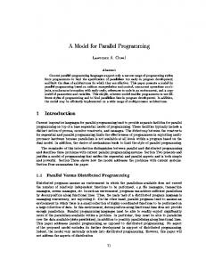
Figure 1: Scenario illustrating propagation of changes from a relational to an XML schema
2. MOTIVATING SCENARIO To motivate the operator definitions that we give in this paper, we will use a scenario that is illustrated in Figure 1 and exemplifies one of the patterns that can be found in many metadata-intensive applications. Consider an e-commerce company that needs to supply its purchase order data to a business partner. The data is stored in a relational database according to a relational schema s1. For the purpose of data exchange, both companies agree to use a common XML schema d1. (The correspondences between the elements of schema s1 and d1 are depicted as light gray lines.) Schema d1 differs from s1 in terms of structure and naming. The relational schema undergoes periodic changes due to the dynamic nature of the business. Assume that s2 is a new version of s1, in which columns “Brand” and “Discount” have been deleted, columns “ShipDate”, “FreightCharge”, and “Rebate” have been added, and column “UnitPrice” has been renamed to “Price”. These changes (highlighted in bold in Figure 1) need to be propagated to the XML schema, so that d1 becomes d2. The change propagation described above can be done as follows. First, the changes introduced by s2 need to be detected, i.e., s1 and s2 need to be matched. Then, the d1 images of the elements deleted in s1 need to be removed from d1. Finally, the XML schema counterparts of the added and renamed columns in s1 need to be merged into d1 to obtain d2. During these steps, intervention of a human engineer may be required, for example, to decide whether the new column “Rebate” should indeed be added to the exchange schema or is not part of the exchanged data and should be omitted. Still, a major portion of the work is mechanical and can be automated. Notice that the procedure sketched above could be applied in the reverse case, when the XML schema d1 is the one that has been modified and the changes are to be propagated back to the relational schema s1. Another instance of the same pattern is round-tripping the modifications from a relational schema like s1 to an existing conceptual schema of the data, which may be expressed as an ER diagram. A key idea of generic model
d1′ = d1 w/o deleted c = converted from s2 c′ = added
s1_d1
s2
ProductID ProductName Brand Quantity UnitPrice Discount
XML schema
PName Brand
OID PID Quantity UnitPrice Discount
d1
c′
c′_d1′
PID
O-DETAILS DID
OrderID OrderDate Employee Customer PONum SalesTaxRate Product
d2 ′_ d1
OrderDate Employee Customer PONum SalesTaxRate
PurchaseOrder
s1_s2
relational schema
OID
PRODUCTS
relational schema
s1
ORDERS
2 _d c′
d2 d1′ c′
Figure 2: Schematic representation of a solution for change propagation scenario of Figure 1 management is to solve such tasks at a high level of abstraction using a concise generic script. Below we present an actual model-management script that implements the above solution for our change propagation scenario, and is directly executable by our prototype. We will use the script to introduce the major model-management operators, which we define in the subsequent sections. To explain the individual steps of the script, we use a schematic representation of the solution shown in Figure 2. The rectangles labeled s1, s2, d1, and d2 represent the four schemas of Figure 1. The arcs between the rectangles denote the mappings between the schemas. For example, the correspondences between schemas s1 and d1 in Figure 1 are shown as a single arc from rectangle s1 to d1 in Figure 2. At the bottom of Figure 2, there is a schema c, which does not appear in Figure 1. To see why it is needed, recall that s1 and d1 are expressed using two different schema languages. The new schema elements added to s1 by way of s2 have no counterparts in schema d1. That is, the new elements need to be converted from the source schema language to the target language. For example, the attribute “ShipDate” added to relation “ORDERS” needs to be converted to a subelement of the complex type “PurchaseOrder” in the XML schema. This step is often referred to as schema translation in the literature. In our solution, we assume that such a translation tool is available as an operator, say SQL2XSD, which takes as input a relational schema and produces as output an XML schema and a mapping between the original and converted schema elements. Thus, the schema c and the mapping s2_c between s2 and c shown in Figure 2 are obtained as 〈c, s2_c〉 = SQL2XSD(s2). Note that schema c is not yet the desired result d2; for example, c may contain an unneeded complex type O-DETAILS, and may differ from d1 structurally. Now, our solution for the change propagation scenario can be expressed as the following script: operator PropagateChanges(s1, d1, s1_d1, s2, c, s2_c) 1. s1_s2 = Match(s1, s2); 2. 〈d1′, d1′_d1〉 = Delete(d1, Traverse(All(s1) − Domain(s1_s2), s1_d1)); 3. 〈c′, c′_c〉 = Extract(c, Traverse(All(s2) − Range(s1_s2), s2_c)); 4. c′_d1′ = c′_c ∗ Invert(s2_c) ∗ Invert(s1_s2) ∗ s1_d1 ∗ Invert(d1′_d1); 5. 〈d2, c′_d2, d1′_d2〉 = Merge(c′, d1′, c′_d1′); 6. s2_d2 = s2_c ∗ Invert(c′_c) ∗ c′_d2 + Invert(s1_s2) ∗ s1_d1 ∗ Invert(d1′_d1) ∗ d1′_d2; 7. return 〈d2, s2_d2〉;
The script defines a generic operator PropagateChanges, which takes six parameters as input (including the converted schema c), and produces two return values 〈d2, s2_d2〉 as output. Below, we explain the script line by line.
1. In line 1, schemas s1 and s2 are “matched” to detect the changes. The result is a mapping s1_s2 shown schematically in Figure 2. Speaking informally, the mapping connects the equivalent elements of s1 and s2. The new elements of s2 (e.g., “ShipDate”) and deleted elements of s1 (e.g., “Brand”) have no matching counterparts, so they remain unconnected. 2. Line 2 illustrates how operators can be combined. First, the deleted elements of s1 are identified using the expression All(s1) − Domain(s1_s2), i.e., all elements of s1 without the matched (and thus not deleted) elements. Then, these elements are used to “traverse” the mapping s1_d1. For example, the deleted relational attribute “Brand” traverses s1_d1 and yields the XML schema element “Brand” of d1. Finally, these d1 images of the deleted elements are removed from d1 using the operator Delete. The result is a new schema d1′ (a “subschema” of d1), and a mapping d1′_d1, which describes how d1′ relates to d1. 3. Line 3 is quite similar to line 2. The new elements of s2, i.e., those missing from the range of s1_s2, traverse s2_c into the converted model c. For example, the image of relational attribute “ShipDate” is an XML schema element “ShipDate” obtained by conversion. A “subschema” c′ containing the images of the new elements is then extracted from c using the operator Extract, which also returns the mapping c′_c. In addition to the elements obtained by traversal like “ShipDate”, c′ contains extra elements of c, such as the complex type that encloses “ShipDate”, to make c′ a well-formed XML schema. Such extra elements are called “support” elements [5]. 4. At this point, d1′ is a subschema of d1 without the deleted elements, and c′ contains the added elements and their support elements. Schemas d1′ and c′ need to be merged to obtain the final result d2 (line 5). As we explain in Section 4.5, the merging of two schemas is driven by a mapping that tells how elements of the two schemas, specifically the support elements of c′, correspond to each other. The mapping between d1′ and c′ is shown in Figure 2 as an arc connecting the two enclosed rectangles. This mapping can be obtained by “composing” the existing mappings between c′, c, s1, s2, d1, and d1′ as c′_c ∗ Invert(s2_c) ∗ Invert(s1_s2) ∗ s1_d1 ∗ Invert(d1′_d1). To get the composition right, mappings s2_c, s1_s2, and d1′_d1 need to be “inverted”, i.e., the domains and ranges of the mappings need to be swapped. 5. The final result of change propagation, schema d2, is computed by the Merge operator. Additionally, the operator returns two mappings, c′_d2 and d1′_d2, which describe how d2 relates to the inputs to Merge, c′ and d1′. 6. As a last step, we compute s2_d2, a new version of the mapping s1_d1 given as part of the input. We need s2_d2 to ensure that our change propagation script can be re-applied if the source schema evolves again. Since d2 is obtained by merging d1′ and c′, the mapping s2_d2 is essentially a union of two mappings, the one between s2 and the d1′-portion of d2, and the one between the s2 and c′-portion of d2. These two mappings can be obtained by composition as s2_c ∗ Invert(c′_c) ∗ c′_d2 and Invert(s1_s2) ∗ s1_d1 ∗ Invert(d1′_d1) ∗ d1′_d2, respectively. Their union is denoted using the plus sign (+). Notice that the above script is not limited to propagating changes from relational schemas to XML schemas. In fact, the reverse
propagation problem can be solved using the same script by assigning the original and modified XML schemas to s1 and s2, and the relational schema to d1. Of course, the input parameters c and s2_c need to be obtained using a different converter, e.g., as 〈c, s2_c〉 = XSD2SQL(s2). In our implementation, every intermediate result of a script such as the one above can be examined and adjusted by a human engineer using a graphical tool. Specifically, the result of Match in line 1 can be post-processed to remove incorrectly suggested matches and add missing ones. Similarly, the merging in line 5 is in general a semiautomatic process, which requires human feedback. Finally, by adjusting the intermediate results of operator compositions in lines 2 and 3 the engineer can decide which additions and deletions should not be propagated. In the above discussion, we introduced several operators informally. To make these operators effective and usable by developers, their semantics needs to be specified precisely. Our goal is to make the semantics as “generic” as possible, so the operators can serve a broad range of model-management tasks. In the next two sections we describe this semantics, first by defining the structures on which they operate, and then by describing the operators themselves.
3. CONCEPTUAL STRUCTURES Model-management applications deal with a wide range of metadata artifacts, which include not only schemas, such as the relational and XML schemas in our motivating scenario, but also view definitions, interface specifications, etc. We represent the formal descriptions, or models, of these artifacts as directed labeled graphs. This graph representation is quite flexible and can accommodate virtually any type of models. We also introduce two additional structures, called morphisms and selectors. Morphisms are binary relationships that establish n:m correspondences between the elements of two models (i.e., nodes of two graphs). For example, in our motivating scenario morphisms are used for keeping track of the XML counterparts of the relational schema elements. Two morphisms, one between s1 and d1 and another between s2 and d2, are shown in Figure 1 using light gray lines. The third conceptual structure, selector, is a set of elements used in models. A major benefit of using selectors is that various operations, in particular the set operations, which would typically produce non-well-formed models if used directly, can be applied to selectors safely. In the following subsections, we define models, morphisms, and selectors as abstract graph and set structures. We also describe them in an equivalent representation as relations. The latter will make it easier to define the semantics of the operators, which follow later.
3.1 Models We represent models as directed labeled graphs. The nodes of such graphs denote model elements, such as relations and attributes in relational schemas, type definitions in XML schemas, clauses of SQL statements, etc. We assume that each element is uniquely identified by an object identifier (OID). A directed labeled graph is a set of edges 〈s, p, o〉 where s is the source node, p is the edge label, and o is the target node1. For a given source s and label p, the target nodes may be sequentially ordered. Their order can be captured by an ordinal property on edges. Thus, 1
The notation (s, p, o) stands for (subject, predicate, object).
CREATE TABLE PRODUCTS ( PID int PRIMARY KEY, PName varchar ) Table type column:1
a1 name
column:2
PRODUCTS
Column SQLtype
int
name
PID
type
a2 type
SQLtype
varchar
name
PName
a3 keyCol
a4
type
S a1 a1 a1 a1 a2 a2 a2 a3 a3 a3 a4 a4
P
O
N
type Table column 1 a2 column a3 2 name “PRODUCTS” type Column SQLtype int name “PID” type Column SQLType varchar name “PName” type PrimaryKey keyCol a2
PrimaryKey
Figure 3: Sample model shown as graph and 4-tuples conceptually a graph can be viewed as a relation M with four attributes, M(S: OID, P: OID, O: OID ∪ Literal, N: integer), where N is an optional attribute used for ordering and S, P, O form a unique key. The node identifiers and edge labels are drawn from the set of OIDs, which can be implemented as integers, pointers, URIs, etc. The literals include strings, integers, floats, and other data types. The type of attribute O is defined as a union type of OIDs and literals. Consider the example in Figure 3. It illustrates how a relational table PRODUCTS defined in SQL DDL (top left) is represented as a graph (bottom left) and as a corresponding set of 4-tuples (on the right). The ovals in the graph denote OIDs, and rectangles denote literals. Nodes a1, a2, a3 represent the table PRODUCTS and its columns PID and PName, respectively. Node a4 represents the primary key constraint on PID. For readability, the identifiers such as Table or Column are spelled out as names rather than opaque IDs. The order of the columns identified by the nodes a2 and a3 is determined by the values 1 and 2 of attribute N (fourth attribute of the table with 4-tuples). In general, the node ordering with respect to a given {src node} and {edge label} is determined by the SQL query: SELECT M.O FROM M WHERE M.S={src node} AND M.P={edge label} ORDER BY M.N. In the example, we have M.S=a1 AND M.P=column. A formal specification of the rules for encoding a model as a graph is called a meta-model. A model is well-formed if it conforms to its meta-model. For example, Figure 3 illustrates a graph encoding of relational schemas that uses specific edge labels, such as SQLtype or name, and auxiliary nodes, such as Table, varchar, or PrimaryKey. If we know the relational meta-model, we can tell whether or not a given graph represents a well-formed relational schema. For example, if we know that each column must have an SQL type, then removing the edge 〈a2, SQLtype, int〉 from the graph in Figure 3 yields a model that is not well-formed. For the purposes of this paper, it is unimportant how a meta-model is represented and how one checks that a model conforms to its meta-model. The details of the graph representation of models remain opaque to the developer of model management applications. Of course, the representation is visible to developers of model management operators. So, a developer must be aware of the representation to implement a custom, non-generic operator, e.g., an operator to normalize relational schemas.
3.2 Morphisms Many metadata-intensive applications, such as data integration and warehousing tools, use a graphical metaphor like the one shown in Figure 1 for representing schema mappings. These mappings are shown to the engineer as sets of lines connecting the
CREATE TABLE PRODUCTS ( PID int, PName varchar )
L
R
a1 a2 a3 a3
b2 b3 b4 b5
Figure 4: Morphism between relational and XML schema elements of two schemas. We call such mappings (schema) morphisms. Thus, a morphism is a binary relation over two (possibly overlapping) sets of OIDs, i.e., a set of pairs 〈l, r〉 drawn from OID×OID. Clearly, a morphism is a weaker representation of a transformation between two models than an SQL view or the mapping languages and expressions suggested in [3,5,14,19,20]. In particular, a morphism carries no semantics about the transformation of instances that conform to the models (e.g., no SQL WHERE-clause). Still, we have found that many mappings can be expressed in this way such as in our change propagation scenario of Section 2. The morphisms have several other advantages. Given our graph representation of models, a morphism can represent a mapping between different kinds of models, e.g., between a relational and XML schema. A morphism can always be inverted and composed. (In contrast, an SQL view cannot be composed with an XSLT transformation in an obvious way.) And since morphisms can be expressed as binary relations, they can be implemented and manipulated easily. Consider the example in Figure 4. The top part of the figure shows the relational schema of Figure 3 and an XML schema. A morphism between the two schemas is depicted graphically as four arcs that connect the elements of the schemas. The bottom part of the figure shows the same morphism represented as a relation. The node identifiers a1, a2, a3 correspond to those of Figure 3. The nodes b2, b3, b4, b5 denote respectively the complex type “Product” and the elements “ProductID”, “ProductName”, and “ProductType” defined in the XML schema (its graph representation is illustrated in Figure 5). Notice that a node can be connected to multiple nodes; e.g. a3 is connected to b4 and b5. Moreover, various kinds of model elements, such as relations or attributes, can participate in a morphism. In an implementation, it may be convenient to annotate the pairs 〈l, r〉 with additional properties. For example, most implementations of the Match operator compute similarity values between the elements of two models. These values can be returned conveniently using a morphism in which each pair has an additional similarity property. Hence, although we define a morphism conceptually as a binary relation H(L: OID, R: OID), it may contain additional attributes, as required by the individual operators. Typically, the L elements originate from one model, and the R elements from another.
3.3 Selectors A selector is a set of node identifiers, which may originate from a single or multiple models. It can be represented as a relation with a single attribute, S(V: OID), where V is a unique key. Figure 6 shows an example of a selector that contains all OIDs used in the model depicted in Figure 3.
schema
tag
complexType
b1 tag
V child:1
b2 name Product
element tag tag tag
child:1
name
b3 type name
b4 type type child:3 b5
child:2
name
ProductID int ProductName string ProductType
Figure 5: Graph representation of XML schema in Figure 4
a1 a2 a3 a4 Table Column PrimaryKey int varchar
Figure 6: Example of a selector
4. OPERATORS In our motivating scenario, we introduced high-level operators whose inputs and outputs are models, morphisms and selectors, such as Match, Delete, Traverse, Extract, and Invert. Such operators raise the level of abstraction of manipulating metadata structures by considering whole models and morphisms at a time, as opposed to node-at-a-time primitives. In this section, we define the precise semantics of these operators on the structures defined in Section 3. Their implementation is covered in Section 5. We start our presentation of operator semantics in Section 4.1 with what we call primitive operators. These are generic operators whose semantics can be defined formally using the relational algebraic manipulation of the relational representations of Section 3. For notational convenience, we express this manipulation in SQL. After that, we introduce the other more powerful operators: such as Extract, Delete, Match, and Merge, whose semantics is more subtle and still a subject of ongoing research. As we will see, some operators, such as Subgraph or Copy, are agnostic about the kind of models passed as input, whereas the semantics of others depends on the underlying meta-model. The GUI operators EditMap and EditSelector allow arbitrary transformations of morphisms and selectors by an engineer. Thus, their semantics cannot be constrained any further.
4.1 Primitive operators Table 1 lists the definitions of seven primitive operators. The left column contains the operator definitions expressed in SQL. Variables m, s, and map hold a model, a selector, and a morphism, respectively. The right column illustrates the application of the operators using simple examples. All primitive operators defined in the table are standard set-theoretic operators. Notice that their definitions are expressed declaratively, i.e., the implementation of these operators, or functional combinations thereof, can be optimized using standard query optimization techniques. The operator Domain extracts the “left” elements from a morphism and returns a selector that holds the result. The operator RestrictDomain restricts a morphism to a smaller element domain, which is specified by the selector passed as a second parameter of the operator. The Invert operator swaps the left and right elements of a morphism. The Compose (∗) operator is defined as the natural join of two morphisms, yielding another morphism. The TransitiveClosure operator on morphisms is specified using a recursive SQL definition. The Id operator creates an identity morphism over a given selector. The operator Subgraph(m, s) extracts from model m a subgraph induced by the nodes referenced in s. The literals attached to the nodes in s are also extracted from m. In the example of Table 1, the literal “PID” is not contained in the input selector s, but the edge 〈a2, name, “PID”〉 is nevertheless returned as part of the result. The extracted subgraph may not be a well-formed model.
That is, it may not be fully connected and may not conform to its meta-model. The set operators Union (+), Difference (−), and Intersection (∩) are another three important primitive operators. We define these on models, morphisms, and selectors by the corresponding set operations on their representation as relations. For example, Union(x, y) := SELECT * FROM x UNION SELECT * FROM y
Note that applying the set operations to well-formed models may produce a model that is not well-formed. Definition
Table 1: Definitions of primitive operators Example
Domain(map) := SELECT DISTINCT map.L AS V FROM map RestrictDomain(map, s) := SELECT * FROM map WHERE map.L IN s Invert(map) := SELECT map.R AS L, map.L AS R FROM map Compose(map1, map2) := SELECT DISTINCT map1.L, map2.R FROM map1, map2 WHERE map1.R = map2.L TransitiveClosure(map) := WITH RECURSIVE TC(L, R) AS (map UNION SELECT DISTINCT TC.L, map.R FROM TC, map WHERE TC.R = map.L) SELECT * FROM TC Id(s) := SELECT s.V AS L, s.V AS R FROM s Subgraph(m, s) := SELECT * FROM m WHERE m.S IN s AND (m.O IN s OR isLiteral(m.O))
a1 b1
Domain( a2 b2
a1 a2
)= a1 b1
RestrictDomain( a2 b2 , a1 a1 b1
Invert( a2 b2 Compose(
a1 b1 , b1 c1 a2 b2
a
a2
)=
Subgraph(M,
a1 b1
b1 a1 b2 a2
)=
b
TransitiveClosure ( b c
Id( a1
)=
)=
)=
a b a
a1 c1
b c c
a1 a1 a2 a2 a2 Column int
)=
Column type
a2
SQLtype int name
PID
where M = model of Figure 3 The last two primitive operators are All and Copy. The operator All(m) returns a selector that contains only those nodes of m that denote the model elements of the model’s meta-model, such as tables or columns in the relational meta-model. For example, for the model of Figure 3 the operator All yields the selector {a1, a2, a3, a4} and filters out all auxiliary nodes, such as Table or PrimaryKey, that are used in the graph encoding. Frequently, it is important to ensure that a given node identifier is used in exactly one model. Furthermore, unique node IDs make it possible to refer to model elements across model boundaries. For these reasons, we use the operator Copy to create a copy of a model m in which the selected node IDs are replaced by new, uniquely created IDs. In the following definition of Copy, the function uniqueOID() generates a unique OID on each call, and the function ifNULL(x, y, z) returns y whenever x is a NULL value, z otherwise. If s=All(m), the output morphism m′_m is a bijection between All(m′) and All(m). Copy(m, s) := m′_m = SELECT uniqueOID(), s.V FROM s; m′ = SELECT ifNULL(T1.L, m.S, T1.L), m.P, ifNULL(T2.L, m.O, T2.L) FROM m, m′_m as T1, m′_m as T2 LEFT OUTER JOIN ON m.S=T1.R, m.O=T2.R; return 〈m′, m′_m〉;
4.2 Derived operators The derived operators are functional combinations of other operators. For example, consider the definitions shown below. operator Range(map) return Domain(Invert(map)); operator RestrictRange(map, selector) return Invert(RestrictDomain(Invert(map), selector)); operator Traverse(selector, map) return Range(RestrictDomain(map, selector)); operator Restrict(map, m1, m2) return RestrictRange(RestrictDomain(map, All(m1)), All(m2));
The Range of a morphism is obtained as the domain of an inverted morphism, by combining the primitive operators Domain and Invert of Table 1. Similarly, RestrictRange is specified in terms of the operator RestrictDomain by first inverting the input morphism, then applying RestrictDomain, and finally inverting the resulting morphism once again. The third operator, Traverse, was used in our motivating scenario for locating the d1 images of the elements deleted from the relational schema s1. To “traverse” the morphism, it is first domain-restricted by the selector, and the range of the restricted morphism is returned as output. The last operator, Restrict, confines the domain and range of a morphism to the elements of two models m1 and m2. Notice that the definitions of the derived operators above are expressed declaratively, allowing the implementations to be optimized.
4.3 Extract and Delete Extracting and deleting portions of models are operations that are heavily deployed in metadata applications. To perform these operations, we propose the generic operators Extract and Delete. The operator Extract is applied as follows: 〈m′, m′_m〉 = Extract(m, s). The inputs are a well-formed model m and a selector s that identifies the set of nodes to be extracted. The output model m′ satisfies the following properties: (i) m′ contains all selected nodes, (ii) m′ is a well-formed model, (iii) m′ is an equally or less expressive model than m, i.e., m can represent all information of m′, and (iv) m′ is a “minimal” model that satisfies (i)–(iii). Condition (ii) may require that unselected “support” elements be included in m′. Condition (iii) can be characterized formally in terms of dominance and information capacity as suggested in [15,19]. The morphism m′_m is an injective function from All(m′) to All(m), i.e., each model element of m′ has at most one counterpart in m. In general, a model may contain implicit information, such as transitive relationships between model elements. In such cases, the result of Extract may need to make such information explicit. For example, consider a class diagram with three classes A, B, C, and two explicit subclass definitions: A is a subclass of B, and B is a subclass of C. Due to condition (iii), Extract(m, {A, C}) should return a class diagram in which A is defined as a subclass of C. This example illustrates that extraction is a rich operation, whose semantics and implementation may be non-trivial. Conceptually, the semantics of the operator Extract(m, s) can be realized using the following algorithm: 1. Create a “closure” of m, i.e., a model m′ in which all implicit information of m is represented explicitly. 2. Assign s′ = s, where s′ is a temporary selector.
3. For each x in s′, extend s′ with elements needed to satisfy conditions (ii) and (iii). 4. Apply 3 until a fixpoint is reached, i.e., s′ does not change. 5. Extract subgraph t′ induced by s′ as t′ = Subgraph(m′, s′). 6. Obtain a “cover” of t′, i.e., a minimal model t that is semantically equivalent to t′. 7. Return Copy(t, All(t)) as result of extraction. Notice that the operator Copy (Section 4.1) returns a model and a mapping. Deleting a selected portion of a model can be defined as extraction of the unselected portion. Thus, we define operator Delete(m, s) return Extract(m, All(m) – s);
Note that the nodes of s that do not represent the model elements of m, i.e., are not members of All(m), have no impact on the result of deletion due to applying All(m) – s.
4.4 Match The purpose of Match is to uncover how two models “correspond” to each other. It takes two models as input and returns a morphism between them. Match is inherently heuristic. So like the previous literature on Match [23], we do not offer a formal definition of what constitutes a correct output morphism. In general, matching two schemas requires information that is not present in the schemas and cannot be fully automated. Hence, a human engineer needs to review and adjust the suggestions produced by an automatic procedure, either in a post-processing step or iteratively.
4.5 Merge To combine two models into one, we utilize the operator Merge, applied as 〈m, m1_m, m2_m〉 = Merge(m1, m2, map). If the input models m1 and m2 are well-formed, Merge should produce a well-formed model m that (i) is at least as expressive as each of the input models, i.e., capable of representing the information contained in both models, and (ii) is “minimal”, i.e., deleting any element makes the model less expressive than one of the input models. The third parameter to Merge is a morphism map that describes elements of m1 and m2 that are equivalent and should be “merged” into a single element in m. The output morphisms m1_m and m2_m identify the counterparts of the elements of m1 and m2 in the merged model m. The conceptual definition of Merge given above does not say anything about the naming and ordering of model elements. For example, it does not prescribe that the attribute names of m1 take precedence over those of m2, or the other way around. These details are not considered to be part of the semantics of Merge because they inherently involve end-user decision making. They are discussed in Section 5.3.
5. IMPLEMENTATION In this section we discuss our implementation of the conceptual structures and operators presented above. We have found that the relations that were used in Section 3 as standard mathematical representation of graphs actually are a convenient implementation structure too. Our graph representation is based on the classical relational data model, in which node identifiers are constants that can be shared across models. We chose a relational approach instead of an object-oriented one (e.g., the one in [5]) to simplify the implementation and specification of the operators, which can often be done using SQL. Our relational graph model is based on the W3C’s Resource Description Framework (RDF).
For encoding relational schemas, XML schemas, and SQL views as graphs we use the following approach. Our meta-model for relational schemas is based on OIM [8]. For example, the model elements of a relational schema comprise tables, columns, and constraints; a table contains an ordered list of columns, each of which has a type; tables and columns carry names; the constraints are specialized into primary key, unique key, non-null, or referential constraints; a referential constraint refers to two columns, one of which is a foreign key and the other is a primary key; etc. Our graph representation of XML schemas builds on XML DOM. The graph representation of SQL views that we deploy is comparable to a parse tree produced by an SQL processor (see Figure 12 in Appendix A). All clauses, statements, alias definitions, functional terms, etc. are represented as separate nodes. A view graph does not replicate the names of attributes and relations used in schemas, but refers directly to the respective nodes in the schema graphs. The output of the primitive operators is defined uniquely in Section 4, except for the operator All, which is implemented differently for each meta-model. For example, for relational schemas the implementation of All is specified as follows: All(m, s) := SELECT m.S FROM m WHERE m.P=type AND m.O IN {Table, Column, PrimaryKey, UniqueKey, NonNull, ReferentialConstraint}
5.1 Extract and Delete To describe our implementation of the Extract and Delete operators we focus on the relational schemas. Consider the schema m shown on the left of Figure 7. The primary key constraints on PID and DID are depicted as horizontal bars underlining the respective attributes. The referential constraint is shown as a line connecting PRODUCTS.PID and ODETAILS.PID. Assume that in the graph representation of m the three constraints are denoted by the nodes c1, c2, and c3, respectively. For brevity, we henceforth refer to the graph nodes representing the attributes of m simply by using their names. Figure 7 illustrates six examples of extraction and deletion. The output morphisms m1_m, …, m6_m are omitted in the figure for compactness. The first example demonstrates extraction of the attribute PName yielding schema m1. Condition (ii) of Section 4.3 ensures that m1 is a well-formed relational schema, i.e., attribute PName belongs to a relation and has a type specification. Applied to relational schemas, condition (iii) requires that the extracted schema contain all constraints present in the original schema that affect the selected elements. For example, extracting the attribute PRODUCTS.PID from m causes the primary key constraint c1 to be extracted as well, yielding the schema m2. Dropping c1 would violate (iii), since it would allow the attribute PID to contain duplicates and thus the original schema m could not represent all information of m2. Analogously, extracting O-DETAILS.PID from m (as schema m4) needs to preserve the referential constraint c2, which in turn requires the presence of PRODUCTS.PID and its primary key constraint c3. Condition (iv) prevents any other attributes from appearing in m4. In our prototype, the implementation of operator Extract(m, s) for relational schemas is based on the conceptual algorithm of Section 4.3. Steps 1 (“closure”) and 6 (“cover”) are equality assignments. Step 3 of the algorithm is implemented as follows: • If s′ contains constraint x, add to s′ all attributes that participate in the constraint definition.
m PRODUCTS PID: int
c1
PName: varchar
c2
m4 = Extract(m, {O-DETAILS.PID}), m5 = Extract(m, { c2 }): PRODUCTS PID: int
O-DETAILS DID: int
c3
PID: int Quantity: int Price: real
O-DETAILS PID: int
m6 = Delete(m, {PRODUCTS.PID, c1 , c2 , O-DETAILS.DID, c3 }): m1 = Extract(m, {PRODUCTS.PName}): PRODUCTS PName: varchar
m2 = Extract(m, {PRODUCTS.PID}), m3 = Extract(m, { c1 }): PRODUCTS
PRODUCTS PID: int O-DETAILS PID: int Quantity: int Price: real
PID: int
Figure 7: Examples of extraction and deletion from a relational schema m (output morphisms not shown). • If s′ contains attribute x, s′ is extended to include (a) the enclosing relation of x, (b) the type definition of x, (c) the referential constraint or non-null constraint for x, (d) the primary key or unique key definition for x, but only when all attributes participating in the key definition are contained in x. In Figure 7, schemas m3 and m5 illustrate the extraction of nodes that denote constraints. To illustrate case (d), consider a relation P(Name, DOB, Addr) with a unique key constraint on (Name, DOB). According to the algorithm, Extract(m, {P.Name}) yields P(Name). The unique key constraint is not included since P.DOB is not selected. Notice that condition (iii) of Extract makes it impossible to delete a constraint on a relational attribute without deleting the attribute definition, or to delete the primary key attribute participating in a referential constraint without deleting its foreign key attribute. For example, consider schema m6 in Figure 7. Selecting PRODUCTS.PID and the constraints c1 and c2 is not sufficient for deleting this attribute, since O-DETAILS.PID is not selected. In [18], we present more flexible operators ExtractMin, DeleteHard, and DeleteSoft, which allow such deletions by providing fewer consistency guarantees than Extract and Delete. Extraction from XML schemas is implemented analogously to the above algorithm. Type references in XML schemas are treated similarly to the referential constraints in relational schemas. Currently, derived types are not supported.
5.2 Match In our prototype, the Match operator takes as input two models of the same kind, e.g., two relational schemas, and returns as output a morphism. We implemented Match using the Similarity Flooding (SF) algorithm, a graph-matching algorithm presented in [17]. The SF algorithm exploits the structure of the graphs to be matched and performs especially well for detecting the differences between two versions of a schema, which is the case in our motivating scenario and many other metadata applications. The SF algorithm takes as input two graphs m1 and m2, and a set of initial similarity values between the nodes of the graphs, expressed as a weighted binary relation seed. Each pair 〈l, r〉 of seed carries a similarity value between zero and one. In a fixpoint computation, the algorithm iteratively propagates the initial similarity of nodes to the surrounding nodes, using the intuition
that neighbors of similar nodes are similar. The output of the algorithm is another weighted binary relation. In Section 3.2 we defined a morphism as a binary relation. To include weights in a morphism, we add to it a third attribute Sim that holds a similarity value for each pair of nodes. The primitive operators in Section 4.1 ignore this extra information. We implement the operator Match as operator Match(m1, m2, seed) multimap = SFjoin(m1, m2, seed); multimap = Restrict(multimap, m1, m2); map = FilterBest(multimap); return 〈map, multimap〉;
The operator SFjoin encapsulates the SF algorithm. As explained in [17], the multimap returned by the algorithm may contain a large fraction of the cross product of the nodes in m1 and m2, and needs to be filtered. The operator FilterBest implements the filter suggested in [17], which exploits the stablemarriage property. In addition to filtering, we restrict the result of the SFjoin operator to the nodes that represent the model elements of m1 and m2 using the operator Restrict (Section 4.2). The input morphism seed is typically obtained using another auxiliary operator NGramMatch(m1, m2), which computes the similarities of literals in m1 and m2 based on the number of n-grams that they have in common. Alternatively, seed can be obtained by composition of morphisms. If seed is omitted, NGramMatch is invoked in SFjoin by default. The above Match implementation returns both the filtered morphism map, and the unfiltered multimap. The morphism map can be adjusted by the engineer using a graphical tool by invoking the operator EditMap on the outputs of Match, e.g., as map = EditMap(map, multimap). The graphical tool allows the engineer to inspect all candidate matches suggested in multimap. The script used above for implementing the Match operator can be easily adapted to call other external schema matchers, which may deploy thesauri, analyze schema annotations, mine samples of instance data, reuse previous match results, etc., to reduce the manual post-processing effort.
5.3 Merge We discuss our implementation of the Merge operator using the example in Figure 8. On the top, two sample models m1 and m2 get merged into m (the output morphisms are omitted). The morphism map is depicted using directed arcs. The direction of each arc establishes a preference between two model elements; when collapsing the two elements, the target element is kept in the output m, whereas the source element is discarded. For example, the attribute PO.OrderDate is kept and ORDER.ODate is discarded. Such preferences are not part of the semantics of the Merge operator (Section 4.5), but are essential for practical deployment. The input morphism map contains an extra attribute Dir to hold the direction of the arcs (→ or ←). Before Merge is executed, a human engineer has a chance to specify the arc direction in a graphical tool by invoking the operator EditMap. The bottom of Figure 8 depicts m1 and m2 as graphs. For brevity, the arc labels, type edges, and literals are omitted (compare to Figure 3). Node x corresponds to relation ORDER, x1 denotes ORDER.ODate, etc. The morphism map is {〈x, y, ←〉, 〈x1, y2, →〉, 〈x2, z1, →〉}. To implement the Merge operator, we developed an algorithm called GraphMerge, which we describe below. Similar to [11,22],
m1
m2
ORDER ODate CName CAddr
m
PO
ORDER
Amount OrderDate
OrderDate CAddr Amount
CUST
CUST
Customer
− y2
x2
x
y1 x3
+
− z1
x
∪ o
x3
o
y1
z y2
z1
− + y2
oo o+ o− +o −o ++ +− −+ −−
priority order for conflict resolution heuristic:
y
x x1
Customer
z
o
+ z1
+−,−+
y2
x
+−
z1
−o
z
o+
+o
y1
x3
Figure 8: Merging two sample schemas the algorithm consists of three conceptual steps: node renaming, graph union, and conflict resolution. 1. In the first step, the graph nodes at the blunt ends of map are renamed to their targets at sharp ends, in both graphs m1 and m2. The result of renaming is shown on the bottom left of Figure 8. Nodes y, x1, and x2 of both graphs have been renamed respectively to x, y2, and z1. 2. In the second step, we do a graph union, i.e., a set union of two sets of edges, and obtain the graph depicted on the bottom right of the figure. This graph is not a well-formed model, because the node z1, which used to represent the attribute CUST.Customer in m2, has now become an attribute of two different relations, x (ORDER) and z (CUST). 3. Such conflicts are resolved in the third and final step of the GraphMerge algorithm. The above conflict is eliminated by deleting either the edge between x and z1, or the edge between z and z1, effectively making Customer an attribute of either relation CUST or relation ORDER in the merged schema. The choice is made by a human engineer. Step 3 is the costliest step of the algorithm, since it requires human feedback. To partially automate conflict resolution, we developed the following heuristic. Observe that in Figure 8 it seems more “natural” to keep the attribute Customer in relation CUST than to move it to ORDER. To generalize this observation, we track the origin of each edge in the merged graph, and assign to each edge a tag, such as +− or o+, which indicates whether each of the nodes incident at the edge was a source node of map (−), a target node (+) of map, or none of the two (o) (these are the only three possible cases assuming that source and target nodes of map are disjoint). For example, the edge 〈x, z1〉 obtained by renaming from 〈x, x2〉 is tagged with +−, since x is a target node and x2 is a source node of map. Analogously, the edge 〈z, z1〉 is tagged with o+, since z does not appear in map at all. If we knew that o+ edges are always preferred over +− edges, then, in a conflict 〈x, z1〉 could be eliminated without asking the engineer. We examined a variety of merge problems in the context of relational schemas, XML schemas, and SQL views, and established empirically a total order among all tag variations, which helps resolve many conflicts automatically in a way that matches human intuition. This order is shown in the middle right of Figure 8. Intuitively, edges between unchanged nodes (oo) are
least likely to be rejected in a conflict, and thus have the highest priority. Similarly, edges incident at + seem more likely to be preferred than those incident at −. Thus, Steps 2 and 3 are realized as follows. First, all edges in the merged graph are sorted by decreasing priority. Then, iteratively, each edge is taken off the top of the sorted list and is appended to an (initially empty) graph G. If appending the edge violates model consistency, it is rejected. Once all edges have been appended, the engineer examines the result and the choices made heuristically, and makes any necessary adjustments. In the above description of the algorithm, we factored out an important aspect, the ordering of nodes within parent. To illustrate how we reestablish a correct order in the merged schema, consider Figure 8. Node y denoting the relation PO is renamed to x. Thus, when merging this node with the original x in m1, we move attributes y1 (Amount) and y2 (OrderDate) to the last position in the merged schema m. However, OrderDate “overrides” ODate, the first attribute in relation ORDER, and should remain at the first position. Hence, in schema m, the resulting order of attributes is OrderDate, CAddr, Amount. The GraphMerge algorithm is summarized below: Algorithm GraphMerge(m1, m2, map) M := m1 ∪ m2; L := empty list; G := empty graph for each edge e in M do rename nodes of e using map; assign tag to e; append e to L; end for sort edges in L by decreasing tag priority; maxN := SELECT max(M.N) FROM M; while L not empty do take edge e=〈s, p, o, n〉 off top of L; if tag(e) one of {“−o”, “−+”, “−−”} then n := n + maxN; if o is literal then continue loop end if end if if exists e′ = 〈s, p, o, n′〉 in G then replace e′ in G by 〈s, p, o, min{n, n′}〉; else if not conflictsWith(〈s, p, o, n〉, G) then append 〈s, p, o, n〉 to G; end if end if end while return G The number maxN is obtained as the highest existing value of the ordinal property N in m1 and m2 (compare Section 3.1). It is used to move the nodes hanging off renamed nodes to the last positions. To test for renamed nodes, we check whether the corresponding edge tag starts with −, i.e., is one of −o, −+, or −−. The literals belonging to such renamed nodes are removed, to ensure that, e.g., the relation corresponding to node x in the merged graph of Figure 8 will be named “ORDER” and not “PO”. The function conflictsWith() checks whether appending a new edge to G causes a conflict. The GraphMerge algorithm can be used for various kinds of models by implementing the function conflictsWith() appropriately. In our prototype, we deploy the algorithm for merging relational schemas, XML schemas, and SQL views. For example, conflict detection for relational schemas checks that relations cannot contain relations instead of attributes, or that attributes cannot be shared among relations, etc. The Merge operator is implemented as follows:
operator Merge(m1, m2, map) G = GraphMerge(m1, m2, map); s = SELECT L FROM map WHERE Dir=”→” UNION SELECT R FROM map WHERE Dir=”←”; m1_G = RestrictDomain(map, All(m1) ∩ s) + Id(All(m1) – s); m2_G = RestrictDomain(map, All(m2) ∩ s) + Id(All(m2) – s); 〈m, m_G〉 = Copy(G, All(G)); return 〈m, m1_G ∗ Invert(m_G), m2_G ∗ Invert(m_G) 〉;
Recall that Merge must also return morphisms from each of its input models to its output model. Thus, after applying GraphMerge to obtain the merged model G, we compute the morphisms m1_G and m2_G. The selector s contains all source nodes of map. For the example of Figure 8, we obtain m1_G as the union of domain-restricted map, {〈x1, y2〉, 〈x2, z1〉}, which maps each renamed m1 node to its new name, and the identity morphism on not renamed nodes, {〈x, x〉, 〈x3, x3〉}. Finally, G is copied to make the node IDs of the output model m unique, and the morphisms m1_G and m2_G are composed with Invert(m_G), so they range over m instead of G. The GraphMerge algorithm does not “invent” new model elements or establish new relationships between the existing elements. Therefore, the operator Merge as implemented above cannot reorganize schemas to resolve structural conflicts. For example, consider two XML schemas, S1 with element FullName and S2 with elements FirstName and LastName. Merging S1 and S2 should ideally create a new complex type Name with subordinate elements FirstName and LastName. Currently, we are working on addressing such structural conflicts by using n-way merges, in which intermediate schemas Sj are used for describing the desired structural transformations. In Section 4.5 we postulated two “semantic” conditions that Merge should satisfy. Our implementation does not automatically ensure that condition (i) holds. For example, the engineer might decide to “override” a non-null constraint on an attribute in one schema S1 by a primary key constraint of the other schema S2, in which case the output model would be less expressive (i.e. more constrained) than S1. Although this flexibility is often desirable in practice, we are working on a more restrictive version of Merge that always guarantees to satisfy (i) and (ii).
6. PROTOTYPE
In this section, we describe our prototype, called Rondo2, in more detail. Its architecture is shown in Figure 9. Its central component is an interpreter that executes scripts. The interpreter can be run from the command line, or invoked programmatically by external applications and tools. Its main task is to orchestrate the data flow between the operators. The operators can be defined either by providing a native implementation, or by means of scripts. For example, a native operator like ReadSQLDDL reads a text document containing the definition of a relational database and creates its graph representation, whereas WriteSQLDDL exports the graph back as text. Similarly, two native operators ReadDb and WriteDb load and store arbitrary graphs in an SQL DBMS. Native operators are defined in scripts using statements like alias ReadSQLDDL ;
Other operators that have been implemented natively include all primitive operators of Section 5, operators that launch GUIs for editing morphisms and selectors, such as EditMap or 2
Rondo: a musical work in which the main theme returns a number of times.
1280
Native operators Compose Domain GraphMerge SFjoin EditMap (GUI) …
ReadDb WriteDb
SQL DBMS
Scripts
Range Match Merge PropagateChan …
Interpreter
600
1370
DB + graph APIs
1500
Generic MM SQL views 11820
XML Schema SQL DDL
graphs SQL tables
files
ReadSQLDDL WriteSQLDDL ReadXSD WriteXSD ReadSQLView WriteSQLView …
File system
Figure 9: Architecture of the prototype EditSelector, schema translation and conversion operators, and the operators SFjoin and GraphMerge. All other operators, such as Range, Match, or Merge, are implemented by scripts presented in the previous sections. The specification of the commonly used native or derived operators can be grouped in a single script and utilized in other scripts using include statements. The interpreter provides a debugging facility that allows examining the execution traces of complex scripts, and supports flexible handling of the input and output parameters of operators. For example, if an operator returns more than one argument (as does our implementation of the operator Match), some of which are not used subsequently (as in script PropagateChanges in Section 2), they can be tacitly ignored. For minimizing the amount of GUI programming needed for visualizing various kinds of models, we used the following technique. We require an operator like WriteSQLDDL to output not only the textual representation of the model, but also a data structure that describes how the terms in the text relate to the model elements, or graph nodes. In this way the schema elements shown in Figure 11 enclosed in boxes are associated with the graph nodes representing those elements, and the GUI operators EditMap and EditSelector can be used in exactly the same way for relational schemas (Figure 11) or SQL views (Figure 12). At the current stage, our prototype supports the basic features of SQL DDL, XML Schema, RDF Schema, and SQL views, and, in preliminary form, UML. To introduce a new modeling language in the prototype, two steps are required. First, the import/export operators need to be provided, which ensure lossless round-tripping from the native format to graphs and back. Second, several callbacks need to be implemented for supporting the operators All, Extract, and GraphMerge. The code breakdown of the prototype is shown in Figure 10. A large share of the implementation effort was due to the graph APIs responsible for in-memory representation and manipulation of graphs and morphisms, and the database support. The key generic model-management functionality comprises less than 7K lines of code. It includes the interpreter (2050), primitive operators (660), SFjoin (1760) and GraphMerge (700) implementations, as well as the generic GUI operators (1400). The non-generic part is essentially divided among the code needed to support SDL DDL, XML schemas, and SQL views. The smallest portion of code is due to converters: XSD2SQL (260), SQL2XSD (250), View2Morphism (90), and Morphism2View (200). The compactness of the converters is mostly due to the fact that they operate on the internal graph representation using expressive queries. The total amount of code in the prototype is below 24K lines. The total scripting code
6800
Converters
Figure 10: Code breakdown in prototype (in lines of code) developed so far is measured in hundreds of lines. The scenarios shown in the paper run in a few seconds on a 600 MHz laptop with 256 MB of memory. Further scenarios that we implemented include a reintegration scenario from the context of version management, iterative merge, a warehousing scenario, in which we extract a subset of the schema that is sufficient to answer a given set queries, and a view reuse scenario. Due to space limitations, we cannot present all of them in this paper. The view reuse scenario is in Appendix A. Among other aspects, it illustrates how views can be merged, presents the GUIs used in our prototype, and demonstrates the use of the operators Morphism2View and View2Morphism.
7. RELATED WORK Many individual aspects of model-management have been studied extensively in the literature, which is too voluminous to cite here. We highlight only some key aspects. In previous work [2,5,11,12,13,19,20,22], schemas were typically represented as graphs whose nodes denote classes of entities that participate in various semantically rich relationships, such as is-a, has-a, functional dependencies, etc. In our approach, the graphs are syntactic structures, whose semantics is opaque to many operators. Morphisms have been used under varying names in many systems, e.g., as schema correspondences in Clio [21]. To our knowledge, selectors have been first introduced in this paper. Past papers on model management reified mappings as models [5,9,22]. One of the surprises of the present work is how much leverage one can get out of simple morphisms. However, morphisms clearly have their limits. Appendix A presents a scenario in which SQL views are used as reified mappings to describe instance transformations. Reified mappings add complexity to scripts and operator implementations. A general treatment of reified mappings is subject of our ongoing work. The operators discussed in [5] include Diff, Enumerate, and Apply. As explained in [18], in Rondo we implemented the operator Diff using extraction of the unmatched portion of one of the input models. Operators Apply and Enumerate are invoked by passing a selector to native Java code. The change propagation script of Section 2 is an alternative realization of the round-trip engineering scenario presented in [5]. A substantial effort has been devoted recently to schema matching. To minimize the amount of manual post-processing, existing schema matching tools deploy various techniques surveyed in [23], such as machine learning [4], etc. In our prototype, we use the structural matcher of [17], which is available for download from the authors’ website. Our definition of the Merge operator was influenced by the schema join operation of [1]. Schema merging has been further addressed e.g. in [11,19,22]. The algorithms suggested there can exploit rich relationship types that are not available in the GraphMerge
algorithm that we developed, and do not take the ordering of model elements into account. Our heuristic deployed in GraphMerge is only an initial step in the challenging research issue of semiautomatic conflict resolution. Schema translation across different modeling languages has been explored e.g. in [2,13]. The techniques presented there could be used for implementing a generic operator for generating one model from another. Currently, we are using a less general approach, in which each converter is implemented as a custom, non-generic operator. To our knowledge, the generic operators Extract and Delete have first been investigated and implemented in this paper. Our algorithm for Extract was inspired by the discussion of schema merging in [11]. The operators presented in this paper are mostly syntactic, just like the conceptual structures, and are expressed as graph transformations. Focusing on syntax allows the operators like Match or Merge to be implemented in a generic fashion for different kinds of models. However, understanding the semantics of these operators is crucial for assessing the correctness of model-management scripts. For example, the effect of applying “syntactic” operators to schemas ultimately needs to be expressed in terms of what these operators do to the instances of these schemas. Conditions (i)–(iv) for the Extract operator (Section 4.3), or (i)–(ii) for Merge (Section 4.5) reflect the semantics of these operators to a limited degree. Algebraic and model-theoretic semantics of model-management structures and operators has been considered in more detail in [1,19], but is still a new and largely unexplored area. Currently we are working on an instancebased characterization of morphism semantics, building on the approach of [16].
8. CONCLUSIONS In this paper we presented a programming platform for model management that implements all generic operators suggested so far in the literature. We explored the use of morphisms and selectors and introduced several novel generic operators. We discussed the operator semantics and the algorithms that we developed for implementing them. We showed that introducing a new model type like SQL DDL schemas in our prototype requires a moderate programming effort, but brings a large new class of model-management tasks within reach. The main conclusions that we draw are the following: 1. One can solve practical problems using the model management operators. 2. The solutions require a relatively small amount of code. 3. One can get very far using a relatively weak representation for models and mappings. Our implementation experience, backed by the in-depth investigation of the individual operations by other researchers, suggests that the question raised in [7] is likely to have a positive answer, i.e., generic metadata management is in fact feasible. Even if we cannot handle subtle and complex cases, if we can solve a large class of non-trivial problems then we are offering a useful programming platform. Still, resolving the debate of [7] to the full extent can be done only by writing scripts for a substantial number of real applications and demonstrating that they work. Other hard challenges remain open. Examples are providing meaningful semantic constraints on operators and proving that certain syntactic transformations “play by the rules”. A salient non-technical challenge is acceptance by the developer
S1
S2
Figure 11: Morphism between sources S1 and S2 community. As with each new programming paradigm, the willingness of engineers to learn a new way of approaching old problems is critical for success of generic model management.
9. ACKNOWLEDGMENTS We thank Gio Wiederhold and the anonymous reviewers for their insightful comments on the paper. We are grateful to Serge Abiteboul, Paolo Atzeni, Stefano Ceri, Alon Halevy, Martin Kersten, Renée Miller, Rachel Pottinger, and Gerhard Weikum for helpful discussions. This work was supported in part by a grant from the Database Group at Microsoft Research.
A. VIEW-REUSE SCENARIO In this appendix, we examine another scenario, which illustrates the use of the operators presented in this paper for addressing a typical data warehousing task. Consider adding a new source S2 to a data warehouse D. Assume that S2 is similar to an existing source S1. The morphism S1_S2 between the two source schemas is shown in Figure 11. Let an existing SQL view vS1_D describe how the instances of S1 populate D. The view vS1_D is depicted in the middle of Figure 12 (the relevant portion of the warehouse schema can be seen in the CREATE VIEW clause). Our goal is to reuse the view vS1_D for importing S2 data into D, i.e., creating the view vS2_D. Conventionally, this problem is solved manually involving a tiresome and error-prone renaming of the attribute and relation names of vS1_D based on the similarities between S1 and S2. In our prototype, we obtain vS2_D using the following script: 1. S1_S2 = Match(S1, S2); 2. S1_D = View2Morphism(vS1_D); 3. S2_D = Invert(S1_S2) * S1_D; 4. vS2_D′ = Morphism2View(S2_D); 5. map = Match(vS2_D′, vS1_D, Invert(S1_S2)); 6. vS2_D = Merge(vS2_D′, vS1_D, map + S1_S2);
First, we match S1 and S2 to determine the correspondences between the schemas. As can be seen in Figure 11, some of the elements of S1 and S2 remain unmatched, whereas others, such as Department.DeptName are matched to two elements, Companies.name and Companies.legalEntity. In Step 2, we extract the morphism S1_D from the view definition vS1_D using a non-generic operator View2Morphism. For example, the morphism S1_D, which is omitted in the figures for brevity, associates the attribute Personnel.Pname with two attributes, Employee.EmpFName and Employee.EmpLName, etc. Next, we compute the morphism S2_D by composition. In Step 4, a “template” view definition vS2_D′ is generated from S2_D using another non-generic operator Morphism2View. It is shown on the
vS2_D′
vS1_D
vS2_D
Figure 12: Merging two SQL views left of Figure 12. Morphism S2_D contains no information as to how the values of the attribute Personnel.Affiliation are obtained from Companies.name and Companies.legalEntity. Therefore, a functional term fct1 is generated in vS2_D′ as a placeholder. In Step 5, the template vS2_D′ and the existing view vS1_D are matched, using as a seed the morphism between S1 and S2. The resulting morphism, after minor manual corrections, is depicted in Figure 12. Finally, in Step 6 both view definitions are merged to obtain vS2_D, shown on the right. Notice that the function symbol fct0 has been correctly replaced by the nested concatenation, whereas fct1 was left as is. The unmatched WHERE clause was borrowed from vS1_D; the attribute references have however been correctly replaced by Companies.cid and Consultants.cid. To achieve that, the morphism map passed to Merge is extended to include S1_S2. The heuristic deployed in the GraphMerge algorithm produces vS2_D fully automatically, due to relative simplicity of the input views.
REFERENCES 1. S. Alagic, P. A. Bernstein: A Model Theory for Generic Schema Management. Proc. DBPL, pp. 228-246, 2001 2. P. Atzeni, R. Torlone: Management of Multiple Models in an Extensible Database Design Tool. pp. 79-95, EDBT 1996 3. S. Bergamaschi, S. Castano, M. Vincini: Semantic Integration of Semistructured and Structured Data Sources, SIGMOD Record 28(1), pp. 54-59, 1999 4. J. Berlin, A. Motro: Database Schema Matching Using Machine Learning with Feature Selection. pp. 452-466, CAiSE 2002
5. P. A. Bernstein: Applying Model Management to Classical Meta Data Problems. pp. 209-220, CIDR 2003 6. P. A. Bernstein, A. Halevy, R. A. Pottinger: A Vision for Management of Complex Models. SIGMOD Record 29(4), pp. 54-63, 2000 7. P. A. Bernstein (moderator), L. Hass, M. Jarke, E. Rahm, G. Wiederhold (panelists): Is Generic Metadata Management Feasible? Panel, pp. 660-662, VLDB 2000 8. P. A. Bernstein, T. Bergstraesser, J. Carlson, S. Pal, P. Sanders, D. Shutt: Microsoft Repository Version 2 and the Open Information Model. Inf. Systems 24(2), p. 71-98, 1999 9. P. A. Bernstein, E. Rahm: Data Warehousing Scenarios for Model Management. pp. 1-15, Proc. Intl. Conf. on Conceptual Modeling (ER) 2002 10. S. Bowers, L. Declambre: On Modeling Conformance for Flexible Transformation over Data Models, Workshop on Transformation for the Semantic Web, July 2002 11. P. Buneman, S. B. Davidson, A. Kosky: Theoretical Aspects of Schema Merging. pp. 152-167, EDBT 1992 12. K. T. Claypool, E. A. Rundensteiner: Sangam: A Framework for Modeling Heterogeneous Database Transformations, ICEIS 2003 13. S. Cluet, C. Delobel, J. Siméon, K. Smaga: Your Mediators Need Data Conversion! pp. 177–188, SIGMOD 1998 14. S. Davidson, P. Buneman, A. Kosky: Semantics of Database Transformations. In B. Thalheim, L. Libkin, Eds., Semantics in Databases, LNCS 1358, pp. 55–91, 1998 15. R. Hull: Relative Information Capacity of Simple Relational Database Schemata. SIAM J. Computing, 15(3), pp. 856-886, Aug 1986 16. J. Madhavan, P. A. Bernstein, P. Domingos, A. Y. Halevy: Representing and Reasoning about Mappings between Domain Models. pp. 80-86, AAAI/IAAI 2002 17. S. Melnik, H. Garcia-Molina, E. Rahm: Similarity Flooding: A Versatile Graph Matching Algorithm and its Application to Schema Matching. ICDE 2002 18. S. Melnik, E. Rahm, P. A. Bernstein. Rondo: A Programming Platform for Generic Model Management (Extended Version). Technical Report, Leipzig University, 2003. Available at http://dol.uni-leipzig.de/pub/2003-3 19. R. J. Miller, Y. E. Ioannidis, R. Ramakrishnan: Schema Equivalence in Heterogeneous Systems: Bridging Theory and Practice. Information Systems 19(1), pp. 3–31, 1994 20. P. Mitra, G. Wiederhold, M. L. Kersten: A Graph-Oriented Model for Articulation of Ontology Interdependencies. p. 86100, EDBT 2000 21. L. Popa, Y. Velegrakis, R. J. Miller, M. A. Hernández, R. Fagin: Translating Web Data. VLDB 2002 22. R. A. Pottinger, P. A. Bernstein: Creating a Mediated Schema Based on Initial Correspondences. IEEE Data Engineering Bulletin, 25(3), Sep 2002 23. E. Rahm, P. A. Bernstein: A Survey of Approaches to Automatic Schema Matching. VLDB Journal 10(4), 2001