National Center for Theoretical Science (NCTS) of Tsing Hua University at. Hsinchu, Taiwan. We are grateful to Richard Hamilton, Tom Mrowka, and. Gang Tian ...
Rotationally symmetric shrinking and expanding gradient K¨ahler-Ricci solitons Mikhail Feldman ∗ University of Wisconsin
Tom Ilmanen ETH-Z¨ urich
†
Dan Knopf ‡ The University of Iowa
1
Introduction
In this paper, we construct several new families of K¨ahler-Ricci solitons and give examples of flowing through a singularity. Our solitons live on complex line bundles over CPn−1 , n ≥ 2, and complement the examples of Cao [Cao96, Cao97] and Koiso [Koi90]. Certain new solitons have initial condition equal to the metric cone Cn /Zk , k > n, endowed with the quotient flat metric. Another new soliton can be combined with one of Cao’s solitons to construct a noncompact Ricci flow that is smooth and self-similarly shrinking for t < 0, becomes a metric cone at at t = 0, and then continues by smooth, self-similar expansion for t > 0, with a change of topology. It has a unique singular point in space and time, at which the Ricci flow implements the flowdown of a CPn−1 to a point. We also present shrinking solitons on certain spaces with orbifold-type point singularities. A solution (M, g(t)) of the Ricci flow ∂ g(x, t) = −2Rc(g)(x, t) ∂t
x ∈ M,
0 ≤ t < T,
(1)
is called a Ricci soliton if there exist scalars σ(t) and diffeomorphisms ψ t such that g(t) = σ(t) ψt∗ (g0 ), 0 ≤ t < T, (2) ∗
Partially supported by NSF grants DMS-0096090 and DMS-0200644. Partially supported by Schweizerische Nationalfonds Grant 21-66743.01. ‡ Partially supported by a vigre Van Vleck appointment at the University of Wisconsin, as well as NSF grants DMS-0202796 and DMS-0328233. †
1
2 where g0 = g(0). For (2) to hold, it is necessary and sufficient that the identity −2Rc(g0 ) = LX g0 + 4λg0 (3) hold for some constant λ and some vector field X on M . In fact X is the initial velocity field of ψt . By rescaling, one may assume that λ ∈ {−1, 0, 1}. 1 These three cases correspond to solitons of shrinking, translating, and expanding type, respectively (see §2.1). If X vanishes, a Ricci soliton is an Einstein metric. More generally, equation (3) is an elliptic system for the pair (g 0 , X). Ricci solitons frequently arise as limits of parabolic dilations about singularities; see for instance [Ha93b, Ha95, Cao97]. Their study yields useful information about singularity formation and other things: for example, Li–Yau–Hamilton differential Harnack inequalities are exact on appropriate solitons; see [Ha88, Cao92, Ha93a]. Now suppose (M 2n , J, g0 ) is a K¨ahler manifold. The basis of the K¨ahlerRicci flow is the remarkable fact that the Ricci flow g(t) remains K¨ahler with respect to the complex structure J. For Ricci solitons, where g(t) = σ(t)ψt∗ (g0 ), g(t) will also be holomorphic with respect to the complex structure ψt∗ (J). It is then natural to impose the constraint that ψ t∗ (J) = J, or equivalently, that the (1, 0) part of X is a holomorphic vector field: ∂X β /∂ z¯α¯ = 0.
(4)
We shall see that (3) and (4) together are equivalent to the complex analogue of (3), namely −2Rαβ¯ = LX h + 4λhαβ¯ (5) for a real vector field X. We call a metric satisfying (5) a K¨ ahler-Ricci solition. Of particular interest is the case where X = grad Q for some real-valued function Q. A Ricci soliton with this property is called a gradient Ricci soliton. In the K¨ahler case, this implies that X is automatically holomorphic; in fact, (3) and (5) become equivalent. We call such a metric a gradient K¨ ahler-Ricci soliton. (See §2.2 for details.) Let us briefly survey some results on the K¨ahler-Ricci flow and its solitons in the compact case. Good background is the monograph [Tia00] or the introduction to [Tia97]. 1
The factor 4 corresponds to a time lapse of 1/4.
1. INTRODUCTION
3
A K¨ahler-Ricci soliton (including a K¨ahler-Einstein metric) can only exist in the canonical case — that is, if the first Chern class c 1 is positive, negative, or zero, and the K¨ahler class [ω] is parallel to c 1 (see §2.3). In this case, [ω(t)] evolves parallel to itself, and the metric (suitably renormalized) may be expected to approach an ideal representative of its K¨ahler class. If c1 is zero or negative, the Ricci flow exists forever and converges (after rescaling) to the unique K¨ahler-Einstein metric in the given K¨ahler class [Cao85] (building on [Yau77, Yau78, Aub76, Aub78]). When c1 > 0, the Ricci flow remains smooth until the volume goes to zero [Cao85]. What does the rescaled metric converge to? The work of Cao, Hamilton and Tian yields the natural conjecture: after pulling back by diffeomorphisms, the rescaled metric converges, in some sense, to a K¨ ahlerRicci soliton. This conjecture addresses the classical Yau problem: to find a K¨ahlerEinstein metric on a given K¨ahler manifold, or an explanation when it is absent. The n = 2 case has now been completely solved. A complex surface with c1 > 0 is CP2 #kCP2 (generic or non-generic) for some 0 ≤ k ≤ 8. For k = 0 and 3 ≤ k ≤ 8, there is a K¨ahler-Einstein metric [Tia87, TY87, Tia90], whereas for k = 1, 2, there is instead a non-Einstein K¨ahler-Ricci soliton [Koi90, WZ02] (see also [Cao96]). This supports the above conjecture. In higher dimensions it is not so simple. For n = 3 there are positive K¨ahler manifolds with no K¨ahler-Einstein metric and no holomorphic vector field, hence no K¨ahler-Ricci soliton [Tia97]. More recently, a holomorphic obstruction to the existence of K¨ahler-Ricci solitons has been announced [TZ99]. For an analytic criterion relating the existence of K¨ahler-Ricci solitons to certain Moser-Trudinger inequalities, see [CTZ02]. So for n ≥ 3 the conjecture cannot be true in a naive sense, but might hold in a weaker form if we allow singularities or at least a change of complex structure in the limit [Tia03, Ha03]. A soliton on a compact K¨ahler manifold is unique modulo the identity component of the holomorphic automorphism group [TZ99, TZ00, TZ01], generalizing the classic result for K¨ahler-Einstein metrics [BM87]. The results of the present paper are also related to the construction of K¨ahler-Einstein metrics on open manifolds; see for example [Cal79, TY90, TY91, TY86, Hit79] and others. Acknowledgements This paper was completed partly while visiting the National Center for Theoretical Science (NCTS) of Tsing Hua University at Hsinchu, Taiwan. We are grateful to Richard Hamilton, Tom Mrowka, and Gang Tian for helpful discussions.
4
1.1
Ansatz and Method
In this paper we pursue an ansatz due to Cao [Cao96] to produce new solitons on line bundles over CPn−1 . First some nomenclature. Let L` denote the total space of the holomorphic line bundle over CPn−1 with twisting number ` ∈ Z, characterized by the equation hc1 , [Σ]i = `, where c1 is the first Chern class of the line bundle and Σ ≈ CP1 is a positively oriented generator of H 2 (CPn−1 ; Z). When ` 6= 0, we can construct L` as follows. Let Zk act on Cn \{0} by z 7→ e2πi/k z. Then the complement of the zero-section of L ` is biholomorphic to (Cn \{0})/Zk with k = |`|. Thus a negative line bundle L −k is obtained by gluing a CPn−1 into (Cn \{0})/Zk at z = 0, whereas the positive line bundle Lk is is obtained by gluing in a CPn−1 at infinity. In particular L−1 (the tautological line bundle) is the blow-up of C n at z = 0. In the negative case, the zero section is an isolated (non-perturbable) complex hypersurface of L−k . We impose a U (n) symmetry according to the following ansatz. We call a soliton trivial if it is Einstein. Assume n ≥ 2. 1.1 Ansatz g shall be a nontrivial U (n)-invariant gradient K¨ahler-Ricci soliton metric defined on (Cn \{0})/Zk . In addition, we require the following boundary conditions: (A) At z = 0, we shall see that (Cn \{0})/Zk is always incomplete. We require that the metric completion is obtained either by adding a CP n−1 smoothly, adding a point smoothly (when k = 1), or adding an orbifold point (when k ≥ 2). (B) At |z| = ∞, we require either that (C n \{0})/Zk is complete, or that the metric completion is obtained by adding a CPn−1 smoothly. These conditions yield complete K¨ahler-Ricci solitons, compact or noncompact with at most a point singularity. Method Here is how we solve it. The rotational symmetry and the gradient condition allow us to reduce equation (3) to a single fourth-order ODE for the K¨ahler potential, whose solution can be expressed in terms of explicit integrals. Two of the constants of integration have no geometric significance and can be ignored. We are left with a two-parameter family of U (n)invariant K¨ahler-Ricci gradient solitons defined locally in C n (and hence in the quotient (Cn \{0})/Zk ). These computations, which are due to Cao, are outlined in §2, §3, and §4.
1. INTRODUCTION
5
In sections §5, §6, and §8, we vary the parameters so that g is defined on all of (Cn \{0})/Zk and matches boundary conditions (A) and (B). Several combinations have already been explored [Koi90, Cao96, Cao97]. See the table at the end of the section for a comprehensive list. We are most interested in the case of L ` , which contains a CPn−1 as zero-section. It is well known that under the K¨ahler-Ricci flow, the volume of a complex subvariety of M evolves in a fixed way depending only on the first Chern class. We apply this principle in §2.3 to establish the following restriction on the possibilities. 1.2 Lemma Suppose g(t) is a K¨ahler-Ricci soliton on L = L ` , ` ∈ Z. Then: (i) if ` > −n, then g(t) must be a shrinking soliton; (ii) if ` = −n, then g(t) must be a translating soliton; (iii) if ` < −n, then g(t) must be an expanding soliton. K¨ ahler Cones To interpret our results, let C n,p denote Cn \{0} endowed with the K¨ahler metric � � ¯ h(z) := |z|2p−2 δαβ¯ + (p − 1)|z|−2 z¯α¯ z β dz α d¯ zβ , z 6= 0, (6)
where p > 0; this comes from the K¨ahler potential P (z) = |z| 2p /p. Let C n,k,p denote the quotient by Zk . The reader may verify that the metric completion C n,k,p is a metric cone with respect to the homotheties z 7→ az, and that all U (n)-invariant K¨ahler cones on (C n \{0})/Zk have this form up to a constant multiple. Note that p = 1 gives a flat metric, with an orbifold-type singularity at the origin if k ≥ 2. More generally, the cone angle around the origin in each complex line is 2πp/k, and the density ratio VolC n,k,p (B1 )/ VolCn (B1 ) is pn /k. It will turn out that soliton metrics satisfying the completeness condition (B) are automatically conelike at infinity: that is, smoothly asymptotic to C n,k,p at infinity for some p.
1.2
Results
We now explore the various cases in turn, including an overview of the already known cases. Expanding solitons (Cn and ` < −n) We begin with the expanding solitons found by Cao on Cn . They provide a forward evolution of the initial cone C n,p for any p > 0. We discuss their construction briefly in §7.
6 1.3 Theorem (Cao [Cao97]) Let n ≥ 2. For each p > 0, there exists a complete homothetically expanding U (n)-invariant gradient K¨ahler-Ricci soliton Ytn,p = (Cn , gp (t)), 0 < t < ∞, p > 0,
with conelike end modelled on C = C n,p . It is unique up to isometry. As t & 0, the metric g(t) converges smoothly to that of C on the complement of the zero section. The metric space Y tn,p converges to C in the pointed Gromov–Hausdorff sense. Our first result is an expanding soliton L −k for any k > n, p > 0. It provides a forward evolution for C n,k,p . The proof is in §5. 1.4 Theorem (Expanding solitons) Let n ≥ 2. For each integer k > n and real number p > 0, there exists a complete homothetically expanding U (n)-invariant gradient K¨ahler-Ricci soliton Ztn,k,p = (L−k , g(t)),
0 < t < ∞,
with conelike end modelled on C = C n,k,p . It is unique up to isometry. As t & 0, the metric g(t) converges smoothly to that of C on the complement of the zero section. The metric space Z tn,k,p converges to C in the pointed Gromov–Hausdorff sense. Besides the above flow, one can always take the quotient of Y tn,p by Zk and consider it to be a forward evolution of C n,k,p. Let us call this quotient Ytn,k,p . It has a persistent point singularity at z = 0 modelled on the orbifold Cn /Zk . Are these singular evolutions really Ricci flows? The singular set has (parabolic) codimension at least 4 for Y tn,k,p and at least 6 for Ztn,k,p . Heuristically, one expects that a singular set of codimension greater than 2 cannot carry a concentration of curvature, and therefore does not disqualify the flow from being a weak solution. Further evidence comes from the static case, where the Gromov–Hausdorff limit of smooth K¨ahler-Einstein manifolds has singularities of codimension at least 4 [CCT97]. So pending a conclusive notion of weak solution, we regard both Y tn,k,p and Ztn,k,p as valid Ricci flows. Let us discuss uniqueness of the initial value problem. For 0 < k ≤ n, the flow Ytn,k,p is the only known forward evolution of C n,k,p (at least according to our Ansatz: see Proposition 9.3). In particular there is no known smooth forward evolution of C n,k,p when 2 ≤ k < n. For k > n, there is nonuniqueness: C n,k,p can flow either by Ytn,k,p or by Ztn,k,p.
1. INTRODUCTION
7
An interesting special case is when p = 1, so the initial condition is the flat cone Cn /Zk . For k > n, besides remaining still, it can begin to move under the Ricci flow. This may seem surprising, since one might expect a flat metric to remain static under the Ricci flow. But this phenomenon is already familiar from other geometric heat flows (such Yang-Mills flow and harmonic map heat flow [Ilm95a, Ilm95b, Fan99, Gas00]). For example: consider 3 possible mean curvature evolutions starting at a cross in R 2 . ... ... .... ... .... .... .... ... . . . . .... . .... .... .... ... .... ...... ........ . . . ... ... .... ...... .... .... ... .... .... .... . . . .... .. . . . .... .... .... . . .
12
.......
3
. ... ...................... ... ...... ............. .. ............. .. .................. ........... ................ ..... .............. ..................... .................... ... .... .......... ......... ... .... . . .. ..... ....... .... . .. . ... ........ ... .. ...... ....... .... . . ... ... ....... ... ... ... .... ...... ......................... .............. ............. ............ ............ ............ .................. . . . ........... ...... .. .
Figure 1. Three mean curvature flows In fact, a stationary cone in Rn has a nonstatic evolution if and only if it is not area minimizing [Ilm95b]. So for Ricci-flat metric cones, we may regard the absence of a nonstatic Ricci flow as a dynamical criterion that substitutes for a minimizing condition. Note that the cross actually has infinitely many mean curvature evolutions, since it may begin moving at an arbitrary time t break ∈ R. Analogously, we expect the singular flow Y tn,k,p to be fragile for k > n in the sense that at any time the orbifold point can spontaneously desingularize to a tiny copy of the expanding soliton Z tn,k,1 , which then grows approximately self-similarly for awhile, and the flow has moved away from Y tn,k,p . Several problems concerning the Ricci evolution of K¨ahler cones appear in §10. Translating solitons (` = −n) Translating solitons were found by Cao on L−n and on Cn [Cao96] by compactifying Cn \{0} at z = 0. In both cases, in the sphere S 2n−1 at metric distance d � 0 from z = 0, the Hopf fibers U (1) · √ z ∼ = S 1 have diameter O(1), whereas the CPn−1 -direction has diameter O( d). As the latter behavior resembles the cigar soliton on C, this asymptotic behavior is called cigar-paraboloid. Shrinking solitons (−n < ` < 0) By contrast with the expanding case, shrinking solitons are relatively hard to produce. For example, there is no U (n)-invariant shrinking soliton metric on C n (Proposition 9.2). The following theorem yields a unique U (n)-invariant shrinking soliton on L −k
8 for each 0 < k < n; the aperture p of the limiting cone at t = 0 is determined by n and k. It is proven in §6. 1.5 Theorem (Shrinking solitons) Let n ≥ 2. For each integer 0 < k < n, there exists a complete homothetically shrinking U (n)-invariant gradient K¨ahler-Ricci soliton Xtn,k = (L−k , g(t)),
−∞ < t < 0,
with a conelike end. It is unique up to isometry. The cone at spatial infinity has the form C = C n,k,p where p = p(n, k). As t % 0, the metric g(t) converges smoothly to that of C on the complement of the zero section. The metric space X tn,k converges to C in the pointed Gromov–Hausdorff sense. Flowing through the singularity By matching the cone angle at t = 0, we may regard Ytn,k,q as a continuation of Xtn,k past the singular time. We concentrate on the case k = 1 since it has the most smoothness. Set q := p(n, 1) and define n,1 t 0.
For t < 0, Nt is biholomorphic to L−1 , has a conelike end, and is homothetically shrinking. At t = 0 the singular fiber (the zero section) pinches off and Nt becomes a K¨ahler cone with an isolated singularity. Then the singularity smooths out: for t > 0, Nt is biholomorphic to Cn , has a conelike end, and is homothetically expanding. A blowdown has occured. Regularity across t = 0 is expressed by the following theorem, proven in §7. 1.6 Theorem (Flow-through) The flow N t is smooth in space-time except for an isolated point singularity at t = 0, and solves the Ricci flow where it is smooth. The smoothness should be understood as follows: for t ≤ 0 the spacetime manifold is W− := (L−1 × (−∞, 0]) \ (L0 × {0})
1. INTRODUCTION
9
where L0 is the zero-section, whereas for t ≥ 0 it is W+ := (Cn × [0, ∞)) \ {(0, 0)}. These glue together along their common boundary C n \{0} at t = 0 to form a smooth space-time manifold W of real dimension 2n + 1 foliated by the spatial hypersurfaces Nt . The assertion of the theorem is that g(x, t) is smooth on W and solves the Ricci flow, and that the metric completion of the spacetime metric g(x, t) + dt2 is obtained by adding just one point. The flow is continuous in the Gromov–Hausdorff topology. This is the first known example for the K¨ahler-Ricci flow of what we call a local singularity: the singularity at t = 0 involves only part of the metric space N0 . In the much-studied canonical case, the manifold shrinks off all at once, presumably to a point (at least, the volume of each analytic cycle goes simultaneously to zero), so a local singularity in the sense expressed here cannot occur. By contrast, in the non-canonical case, various parts shrink or grow at different rates, like jangling springs, so local singularities must occur in some cases. See Example 2.2. Similar phenomena — shrinking and expanding solitons, flow-through with a point singularity at t = 0, and the relative difficulty of finding shrinking solitons as against expanding ones — occur for other geometric heat equations, including mean curvature flow [ACI95, AIV, Ilm95b], harmonic map heat flow [Ilm95a, Ilm95b, Fan99, Gas00], Yang-Mills heat flow [Gas00], and the equation ut = ∆u+up [Tro87, BQ89, Lep90]. Related examples exist for nonlinear wave equations [STZ94] and nonlinear Schr¨odinger equations [Mer98]. Compact shrinking solitons There is no complete soliton on L k , k > 0, (Proposition 9.1). Indeed, the soliton metric is always incomplete at z = 0, and completing it leads to compact solitons in two ways. Let Fk denote the k-twisted projective line bundle CP 1 ,→ Fk → CPn−1 of Calabi [Cal82]. It is obtained from L k by adding a CPn−1 at z = 0 (or equivalently from L−k by adding a CPn−1 at infinity). Shrinking solitons are known to exist on Fk , 0 < k < n [Koi90, Cao96]. There can be no soliton on Fk for k ≥ n because then the CPn−1 at infinity shrinks, whereas the CPn−1 at z = 0 does not. See Lemma 1.2 and Example 2.2. Let Gk denote the compact space Lk ∪ {0}. Note that Gk = CPn /Zk branched over z = 0 and over the CPn−1 at infinity (when k ≥ 2). We have the following theorem.
10 1.7 Theorem (Shrinking Orbifolds) For each k > 0, there is a U (n)-invariant shrinking gradient K¨ahler-Ricci soliton metric on G k , k > 0. In the k = 1 case this is just the Fubini-Study metric on CP n . For k ≥ 2 it has an orbifold-type singularity at z = 0 modelled on C n /Zk . For k > n we expect that the flow is fragile: it can spontaneously desingularize to F k via a small, but growing copy of (nearly) Z n,k,1 at the orbifold point.
1.3
Table of solitons
We list all known gradient K¨ahler-Ricci solitons arising as the metric completion of a U (n)-invariant ansatz on (C n \{0})/Zk , n ≥ 2, k > 0 under various closing conditions. We have excluded familiar Einstein manifolds and examples with singularities of real codimension 2. We allow point singularities. (‡) indicates that solitons with point singularities can be obtained as a metric quotient, so they are not separately listed. (1) indicated a 1-parameter family of solitons parametrized by the cone aperture p. In the remaining cases there is a single soliton for each k and n.
2. BEHAVIOR OF SOLITONS
2
11
Topology and type
k-fold symmetry
Behavior as z → 0
Behavior as |z| → ∞
Source
L−k noncompact expanding
n + 1, . . .
smooth CPn−1
conelike (1)
present paper
Cn (‡) noncompact expanding
1
smooth point
conelike (1)
[Cao97]
L−n noncompact translating
n
smooth CPn−1
cigarparaboloid
[Cao96]
Cn (‡) noncompact translating
1
smooth point
cigarparaboloid
[Cao96]
L−k noncompact shrinking
1, . . . , n − 1
smooth CPn−1
conelike
present paper
Fk compact shrinking
1, . . . , n − 1
smooth CPn−1
smooth CPn−1
[Koi90] [Cao96]
Gk compact shrinking
2, . . . , n − 1
orbifold point
smooth CPn−1
present paper
Behavior of solitons
In this section we derive the equations for a gradient K¨ahler-Ricci soliton, establish the conservation laws that rule the growth of volume, and apply it to the bundle L` .
12
2.1
Ricci solitons
Let us show that (1) and (2) are equivalent to (3). First suppose that (M n , g(t)) is a solution of the Ricci flow (1) having the special form (2). We may assume ψ 0 = id and σ(0) = 1. Then ∂g = σ 0 (0) g0 + LY0 g0 , −2Rc(g0 ) = ∂t t=0
where Yt is the family of vector fields generating the diffeomorphisms ψ t . So g0 satisfies (3) with X = Y0 . Conversely, suppose that g0 satisfies (3). Set σ(t) := 1 + 4λt,
and let ψt denote the diffeomorphisms generated by the time-varying vector fields 1 Yt (x) := X(x), ψ0 = id . σ(t) (We assume that X is a complete vector field. This will be always hold in our examples: see (22), (23).) Set g(t) := σ(t)ψt∗ g0 . Then g(t) has the form (2). To see that g(t) is a solution of the Ricci flow (1), calculate ∂g = σ 0 (t)ψt∗ (g0 ) + σ(t)ψt∗ (LYt g0 ) ∂t = ψt∗ (4λg0 + LX g0 ) = ψt∗ (−2Rc(g0 ))
by (3)
= −2Rc(g). This proves (1), and the desired equivalence.
2.2
Ricci solitons on K¨ ahler manifolds
Let (M, g, J) be K¨ahler. Note that g and Rc are real and J-invariant, and ¯ so their αβ and α ¯ β¯ parts vanish. The Hermitian metric h = h αβ¯ dz α d¯ z β is given by h := g − iω := g − ig(J·, ·),
2. BEHAVIOR OF SOLITONS
13 ¯
and the Hermitian Ricci tensor R = Rαβ¯ dz α d¯ z β by2 R := Rc − iρ := Rc − iRc(J·, ·). Now consider the complex soliton equation, namely −2Rαβ¯ = LX hαβ¯ + 4λhαβ¯ ,
(5)
where X is a real vector field. By taking the real and complex parts, this is equivalent to the conjunction of −2Rc = LX g + 4λg
(3)
−2ρ = LX ω + 4λω.
(3i)
and Now (3) and (3i) differ only by a term involving L X J, and by taking the difference, we quickly deduce that X is holomorphic. Conversely, if we assume (3) together with LX J = 0, we deduce (3i). So (5) is equivalent to (3) together with the statement that X is holomorphic, as claimed in the introduction. This is what we call a K¨ahler-Ricci soliton. On the other hand, from (3) alone we can only deduce that ∇ α Xβ + ∇β Xα = 0, which does not quite say that X is holomorphic. But when X is a gradient, the symmetry of ∇α Xβ makes X automatically holomorphic. In detail: assume (3) and let X i = g ij Dj Q with Q real. Then LX g = 2D 2 Q, and (3) becomes −2Rc = 2D 2 Q + 4λg. (7) The Hessian decomposes as ¯ + ∇∇Q ¯ ¯ 2 Q, D 2 Q = ∇2 Q + ∇∇Q +∇ ¯ is the decomposition of the connection into complex and where D = ∇ + ∇ anti-complex parts. Since (7) is real, it suffices to consider only the αβ and αβ¯ components. Then (7) is equivalent to ¯ ¯Q + 2λh ¯ , −Rαβ¯ = 2∇α ∇ β αβ
0 = ∇α ∇β Q.
The second of these yields by conjugation � � ¯ α¯ X β = ∇ ¯ α¯ 2hβ¯γ ∇γ¯ Q = 0 ∇
(8)
(9)
¯ Note that R is double the αβ¯ component of Rc, while ω = (i/2) hαβ¯ dz α ∧ d¯ z β and ¯ ρ = (i/2) Rαβ¯ dz α ∧ d¯ z β . For us σ ∧ ν := σ ⊗ ν − ν ⊗ σ. 2
14 where X β is the complex part of X. So the flow vector of a gradient Ricci soliton on a K¨ahler manifold is holomorphic, as claimed. In local coordinates z = (z 1 , . . . , z n ) the metric can be represented by a K¨ahler potential P : U ⊆ M → R via hαβ¯ =
∂2P . ∂z α ∂ z¯β¯
(10)
The Hermitian Ricci curvature equals 3 Rαβ¯ = −2
∂2 log det h. ∂z α ∂ z¯β¯
¯ depends only on the complex structure and is given in The operator ∇∇ coordinates by 2 ¯ ¯Q = ∂ Q . ∇α ∇ β ∂z α ∂ z¯β¯ So we can write the first equation of (8) as ∂2 (log det h − Q − λP ) = 0. ∂z α ∂ z¯β¯ We are interested in the case of expanding or shrinking solitons, so we take ¯ if necessary, we λ = ±1. Modifying P by an element in the kernel of ∇ ∇ may assume Q = log det h − λP. (11) The operator ∇ is independent of the connection on vector fields of type (1, 0), and (9) takes the form � � ∂ β¯ γ ∂ h Q = 0. ∂ z¯α¯ ∂ z¯γ¯ Inserting Q, we obtain � � ∂ β¯ γ ∂ h (log det h − λP ) = 0. ∂ z¯α¯ ∂ z¯γ¯
(12)
In turn, this equation implies (9) and (8). So h will be a gradient K¨ahlerRicci soliton if and only if h possesses a K¨ahler potential P that satisfies (12). Note that this is a fourth-order equation in P . 3
This corresponds to ρ = −i∂ ∂¯ log det h.
2. BEHAVIOR OF SOLITONS
2.3
15
Conservation laws
We recall the well-known principle that the K¨ahler class evolves in a fixed way, which yields an exact prediction of the volume of complex varieties at any time t. We give two examples, and prove Lemma 1.2. On a K¨ahler manifold, the Ricci flow becomes ∂ω = −2ρ. ∂t Thus the K¨ahler class [ω] in H 2 (M, R) evolves by [ω(t)] = [ω0 ] − 2t[ρ] = [ω0 ] − 4πtc1 ,
(13)
where c1 = c1 (T M ) is the first Chern class of M and [ρ] = 2πc 1 . Let Σ be a complex curve in M . By integrating ω(t) over Σ, we find the following exact prediction for area, |Σ|t = |Σ|0 − 4πthc1 , [Σ]i. If c1 is positive on Σ, then in principle, Σ will disappear at the formal vanishing time |Σ|0 . T (Σ) := 4πhc1 , [Σ]i We call this phenomenon the robot behavior of vanishing cycles. Clearly g(t) must develop a singularity at or before time T (Σ). Suppose that g(t) is a Ricci soliton. Then [ω(t)] = σ(t)[ψt∗ (ω0 )] = σ(t)[ω0 ],
σ(t) = 1 + 4λt,
since a cohomology class is unchanged under a flow by diffeomorphisms. Combining with (13) (or just taking the homology class of (3i)) yields λ[ω0 ] = −πc1 .
(14)
If M is compact, this falls under the canonical case, as mentioned in the introduction. We give two examples. 2.1 Example (Proof of Lemma 1.2) Let L denote L ` , and denote its zero-section by L0 ∼ = CPn−1 ⊆ L. We compute the first Chern class of the complex manifold L. We have T L|L0 = T L0 ⊕ N L0 ∼ = T L0 ⊕ L
16 where N L0 is the normal bundle of L0 in L. By the Whitney product formula, we have in H 2 (L0 , Z), i∗ (c1 (T L)) = c1 (T L|L) = c1 (T L0 ) + c1 (L), where i : L0 ,→ L is the embedding. Let Σ ⊆ L0 be a CP1 that generates H2 (L0 , Z) ∼ = Z. Then hc1 (T L), [Σ]i = hc1 (T L0 ), [Σ]i + hc1 (L), [Σ]i = n + `.
(15)
(A suitable reference is [GH78], Chapter 3, §3.) Integrating (14) over Σ, we obtain λ|Σ|0 = −π(n + `). (16) Thus the sign of λ must be opposite to the sign of n + `. This proves Lemma 1.2. 2.2 Example Let Fk be the k-twisted CP1 bundle over CPn−1 described above. How does it evolve with an arbitrary starting metric? Let Σ0 be a CP1 in the zero-section (at z = 0), let Σ∞ be a CP1 in the ∞-section, and let T be a fiber. Then H 2 (Fk , Z) ∼ = Z ⊕ Z is generated by [Σ0 ] and [T ], and one can compute [Σ0 ] + k[T ] = [Σ∞ ]. From (15) we have for c1 = c1 (T Fk ) hc1 , [Σ0 ]i = n − k,
hc1 , [Σ∞ ]i = n + k,
hc1 , [T ]i = 2.
First consider the case 0 < k < n. Then the areas of all three curves shrink at fixed rates; but which one shrinks off first? This depends on the initial metric only through the ratio of the areas |Σ 0 | and |T |, and there are three possibilities. (1) If |Σ0 |/|T | = (n − k)/2 (canonical case), we believe that the entire manifold remains smooth until it shrinks to a point (a global singularity) and is asymptotic to a shrinking soliton on F k as presented in [Koi90, Cao96]. (2) If |Σ0 |/|T | > (n − k)/2, then T shrinks before Σ 0 . In fact, all the fibers have the same area, and it is reasonable to conjecture that the manifold remains smooth until the final instant, when it converges as a metric space to CPn−1 .
3. THE ODE FOR ROTATIONALLY INVARIANT SOLITONS
17
(3) The evolution is most interesting in the case that |Σ 0 |/|T | < (n−k)/2, so that Σ0 shrinks first. We conjecture the following evolution: as the zerosection shrinks, there forms around it a local singularity modelled on the shrinking soliton Xtn,k of Theorem 1.5. At the singular time, the zero-section shrinks to a point and the manifold develops a cone singularity. If k = 1, the singularity heals smoothly as in Theorem 1.6, the manifold becomes CPn , and eventually shrinks to a point with the Fubini-Study metric. If 2 ≤ k < n, the space becomes Gk with a persistent orbifold singularity, and eventually shrinks off self-similarly to a point, with a singularity modelled on the soliton of Theorem 1.7. See §10 for further questions. In the case k > n, Σ0 expands in area, so the only possibility is that the fiber shrinks first as in case (2) above.
3
The ODE for rotationally invariant solitons
In this section we reduce the K¨ahler-Ricci soliton equations in the U (n)invariant case to an ODE which we can solve nearly explicitly. Our calculations follow those of Cao [Cao96]. In the final part we give a lemma of Calabi that addresses the closing condition at z = 0.
3.1
U (n)-invariant metrics on Cn \{0}
Let h be a U (n)-invariant K¨ahler metric on C n \{0}. Because H 2 (Cn \{0}) = 0, by the ∂-Poincar´e lemma we may assume that the representation (10) holds on all of Cn \{0}. Averaging the potential P with respect to action of U (n), we may assume that P is also U (n) invariant and thus SO(2n) invariant. So we may write P = P (r), where r := log |z|2 . Define φ := Pr ,
(17)
and compute from (10) ¯
h = [e−r φ δαβ¯ + e−2r (φr − φ)¯ z α¯ z β ] dz α ⊗ d¯ zβ .
(18)
The associated Riemannian metric is g = φ (gS 2n−1 − η ⊗ η) + φr (dr ⊗ dr/4 + η ⊗ η) = φ gFS + φr gcyl ,
(19)
18 where η restricts to the 1-form dθ on each complex line, g FS is the pullback of the standard Fubini-Study metric of CPn−1 to Cn \{0}, and gcyl restricts to a round cylinder metric on each punctured complex line. Note that the size of gF S is such that the area of a CP1 in CPn−1 is π. From this formula it is clear that h is positive definite, hence a K¨ahler metric, if and only if φ>0
3.2
and
φr > 0.
(20)
U (n)-invariant gradient K¨ ahler-Ricci solitons
We now specialize (12) to the case of U (n)-invariant solitons on C n \{0}. In this section we will solve the equation locally, and in the next three sections impose particular boundary conditions at z = 0 and at infinity. Substituting equations (17) and (18) into (12), we obtain after some computation the fourth-order ODE Prrrr − 2
2 P3 Prrr 2 + nPrrr − (n − 1) rr2 + λ(Prrr Pr − Prr ) = 0. Prr Pr
(21)
Thus one should in principle expect four arbitrary constants. We shall see that only two of these are geometrically significant. Rather than work with (21) directly, it is easier to perform the following reduction: taking Q = log det h − λP as in (11), one observes that X β = 2hβ¯γ
Qr β ∂Q =2 z , ∂ z¯γ¯ Prr
(22)
so X is holomorphic if and only if there is µ ∈ R such that Qr = µPrr .
(23)
This is a third-order equation for P , and µ is the first arbitrary constant. We write this as a second-order equation for φ ≡ P r : (log φr )r + (n − 1)(log φ)r − µφr − λφ − n = 0.
(24)
(The reduction can also be accomplished by the standard method of rewriting (21) as an exact differential; indeed, one recovers (21) by solving (24) for µ and differentiating.) We shall assume in what follows that µ 6= 0, since otherwise grad Q = 0 and (8) forces h to be an Einstein metric, which we have excluded.
4. CLOSING CONDITIONS
19
Since φr > 0, we can regard r as a function of φ and write φ r = F (φ). A computation yields that F satisfies the linear equation � � n−1 0 − µ F − (n + λφ) = 0. (25) F + φ We solve this to find φr = φ1−n eµφ (ν + λIn + nIn−1 ),
(26)
where ν is the second arbitrary constant and Z Im := φm e−µφ dφ. After integrating by parts and doing a wee bit of algebra to find I m , we write (26) as the separable first-order equation n−1
φr = F (φ) :=
λ λ + µ X n! j j+1−n νeµφ − φ − 1+n µφ . n−1 φ µ µ j!
(27)
j=0
We may integrate this to get an implicit solution r = r(φ). (In low dimensions, the integration can even be carried out.) The third arbitrary constant arises during this integration and represents translation in r, hence dilation in z. The fourth arises when one integrates φ to get P . The third and fourth constants are not geometrically significant. The geometric degrees of freedom reside in µ and ν.
4
Closing Conditions
In this section we show how to add a CPn−1 to (Cn \{0})/Zk at zero or at infinity, or add a point at zero. We postpone the conelike condition at infinity to sections §5 and §6. The following lemma is an immediate consequence of (25). It gives an overview of the zeroes of F . 4.1 Lemma (Zeroes of F ) If φ 6= 0 is a zero of F , then F 0 (φ) = n + λφ.
(28)
Consequently, (1) If λ = 1, then F has at most one positive zero a. (2) If λ = −1, then F has at most two positive zeroes. It has at most one zero 0 < a ≤ n and at most one zero b ≥ n.
20
4.1
Adding a CPn−1 at zero or infinity
We derive the condition for adding a CPn−1 smoothly to (Cn \{0})/Zk . As we shall see, this corresponds to a positive, simple zero of F . The sign of F 0 determines whether it is added at z = 0 or |z| = ∞. Let us start with z = 0. Assume that g is a U (n)-invariant expanding or shrinking gradient soliton defined on a neighborhood of the zero section of L−k , k > 0. Then φ exists for −∞ < r < r0 , and φ > 0, φr > 0 by (20). Let a := lim φ(r). r→−∞
By (19), any CP1 in the zero-section has area |Σ|g = πa > 0. Thus the Robot Principle (16) yields a = k − n,
k>n
a = n − k,
expanding case,
0 0.
Let φ be a solution of φr = F (φ) with φ&a
as
r → −∞
(31)
The ODE is conjugate by a smooth diffeomorphism ψ = Φ(φ) to the equation ψr = βψ, so φ has the form φ(r) = a + eβr A(eβr )
(32)
as φ → a, where A is a smooth function defined on (−ε, ε) with A(0) > 0. In addition |φr (r)| ≤ Ceβr
4. CLOSING CONDITIONS
21
as r → −∞, so by (19), the metric distance to z = 0 is Z
0
−∞
Z p C φr dr ≤
0
∞
Ceβr/2 dr < ∞,
(33)
and the metric is incomplete near z = 0. Integrating (32) in r, the K¨ahler potential P has the form P = ar + f (eβr ) = 2a log |z| + f (|z|2β ),
(34)
where f is smooth at zero, f 0 (0) = A(0)/β > 0. The metric completion of (Cn \{0})/Zk at z = 0 is obtained by adding a CPn−1 . Each complex line through the origin acquires a cone singularity with central angle 2πβ/k. The following lemma tells that the induced metric is indeed smooth when β = k. 4.2 Lemma (Calabi [Cal82]) When β = k, the K¨ahler potential (34) induces a smooth K¨ahler metric on a neighborhood of the zero-section in L−k . Proof. We will use the fact that f is smooth at zero and f 0 (0) > 0. Recall from (19) that h = Pr hF S + Prr hcyl =: h1 + h2 on (Cn \{0})/Zk . We aim to show that h extends smoothly to L := L −k . Now h1 is smooth, since h1 = a hF S = a π ∗ (h0 ), where h0 is the Fubini-Study metric on CPn−1 and π : L → CPn−1 is the projection. We write h2 as ¯ 2, h2 = ∇∇P
where P2 (z) := f (ekr ) = f (|z|2k ) is considered as a function on (Cn \{0})/Zk . It suffices to show that P2 extends to a smooth function on L. It is possible to choose a smooth (nonholomorphic!) local coordinate w : π −1 (U ) ⊆ L → C over U ⊆ CPn−1 which is complex linear on fibers, with the property that |w| = |z|k , that is, |w(p(z))| = |z|k for z ∈ Cn \{0}, where p : Cn \{0} →
22 L\L0 is the canonical k-fold cover. In particular, |w| 2 is a smooth function on L (in fact, it is a bundle metric) and ekr = |z|2k = |w|2 , so P2 = f (|w|2 ) defines a smooth function on L. Thus h extends smoothly to L. Along the zero section, h = ah0 + kf 0 (0) dw dw, ¯ so h is positive and therefore K¨ahler. q.e.d. Now set a := λ(k − n) > 0 as required in (29), and let φ be a solution of φr = F (φ) with φ & a as r → −∞ as in (31). Does the corresponding metric g actually compactify smoothly at z = 0? From (29) and (28) we deduce β = F 0 (a) = n + λa = n + k − n = k, so by Lemma 4.2, g does indeed induce a smooth metric on a neighborhood of the zero-section of L−k . (This is not a coincidence: a dirac of curvature along the CPn−1 would be a source term in the conservation law (13).) A development similar to the above can be given for the case |z| = ∞, F (b) = 0, F 0 (b) < 0, producing a metric on Lk . We summarize both results as follows. 4.3 Lemma Let k > 0. (1) A solution of φr = F (φ) with φ & a as r → −∞ induces a smooth metric on a neighborhood of the zero section of L −k if and only if a = λ(k − n) > 0, and F (a) = 0 or equivalently ν = ν aλ (µ). It is an expanding soliton for k > n, shrinking for 0 < k < n. (2) A solution φ of φr = F (φ) with φ % b as r → ∞ induces a smooth metric on a neighborhood of the zero section of L k if and only if b = k+n > 0 and F (b) = 0, or equivalently ν = νb−1 (µ). It is a shrinking soliton.
4.2
Adding a point at z = 0
We derive the condition for adding a point smoothly to C n \{0} at z = 0. Heuristically speaking, this corresponds to passing the cross-sectional area a → 0 in the above construction. So suppose φ represents a smooth soliton defined on a neighborhood of z = 0 in Cn . Then φ → 0 as r → −∞. We may write F as n−1
ν0 (µ) X µj φj λφ νeµφ − , F (φ) = n−1 − n−1 φ φ j! µ j=0
4. CLOSING CONDITIONS
23
where in agreement with (30), ν0 (µ) :=
n!(µ + λ) . µn+1
F (φ) ≈
ν − ν0 (µ) φn−1
Then
near φ = 0. If ν < ν0 (µ), then F < 0 on 0 < φ ≤ ε, contradicting φ r > 0. If ν > ν0 (µ), then φ reaches 0 at some finite point r 0 > −∞, contradicting existence of φ as r → −∞. We deduce that ν = ν0 (µ). Conversely, let us set ν = ν0 (µ). Then F simplifies to F (φ) = φ + ν0 (µ)
∞ X µj+n−1 φj , (j + n − 1)! j=2
which is smooth at φ = 0 with F (0) = 0, F 0 (0) = 1. So there exists a solution φ of φr = F (φ) defined on some interval (−∞, r 1 ] with φ > 0, φr > 0, and φ & 0 as r → −∞. Since F 0 (0) = 1, the same argument as for (32) shows that φ(r) = er K(er ) where K is smooth at 0, K(0) > 0. Then the K¨ahler potential P satisfies P = er L(er ) = |z|2 L(|z|2 ), where L is smooth at 0, L(0) > 0. Thus P induces a smooth K¨ahler metric on a neighborhood of 0 in Cn . We have proven the following Lemma. 4.4 Lemma Let k = 1. A solution of φr = F (φ) induces a smooth metric on a neighborhood of 0 in Cn if and only if F (0) = 0, that is, if and only if ν = ν0 (µ).
24
5
Expanding solitons on line bundles
In this section we construct a 1-parameter family of expanding solitons on L−k for each k > n, thereby proving Theorem 1.4. The closing condition at z = 0 reduces the parameter space (µ, ν) by 1 dimension. Completeness as |z| → ∞ comes for free. The solution is asymptotic to a cone at spatial infinity, and therefore this cone is also the initial condition of the expanding flow defined for t > 0. Any cone aperture p > 0 can be realized. Proof of Theorem 1.4. 1. We first show existence. Set λ = 1. By Lemma 4.3, the closing condition at z = 0 can be satisfied if and only if we set ν = νa+1 (µ), a = k − n > 0. For each µ 6= 0, we obtain a solution of φ r = F (φ) defined on a maximal interval −∞ < r < r1 , such that F (a) = 0 and φ & a as φ → −∞, and a corresponding expanding soliton defined on a neighborhood of the zero section of L−k . For each µ, φ is unique up to translation and g is unique up to isometry. For λ = 1, (27) becomes n−1
φ 1 + µ X n! j j+1−n νeµφ µφ . φr = F (φ) := n−1 − − 1+n φ µ µ j! j=0
By Ansatz 1.1, we wish φ to be defined for all −∞ < r < ∞. Now recall from Lemma 4.1 with λ = 1 that a is the only positive zero of F , and F > 0 on (a, ∞). Thus φ increases without bound as r converges to its maximal value r1 ≤ ∞. Now if µ > 0, then examining (30) with λ = 1, we find that ν > 0, so φr = F (φ) is dominated by the superlinear term νφ 1−n eµφ > 0 for large φ. This implies that r1 < ∞ which contradicts the Ansatz. We previously excluded µ = 0. Thus we have proven the following additional necessary condition. 5.1 Lemma An expanding soliton on L−k must have µ < 0. Conversely, assume that µ < 0. Then the exponential term in F (φ) becomes tame, and the dominant term for large φ is the linear term −φ/µ > 0. This implies that φ exists for all −∞ < r < ∞. Note that the conditions φ > 0, φr > 0 of (20) are satisfied automatically and we get a K¨ahler metric. It is an expanding soliton on L−k .
5. EXPANDING SOLITONS ON LINE BUNDLES
25
2. We next verify that L−k is conelike at infinity and in particular complete. We may write φr = F (φ) in the form � � φ 1 φr = − + G , µ φ where G is smooth at zero. Rewriting the equation in terms of ψ := 1/φ and invoking the principle used in (32), we find that φ(r) = e−r/µ B(er/µ ),
(35)
for large r, where B is smooth and B(0) > 0. Comparing with the K¨ahler cone potential |z|2p /p following (6), we see that g is spatially asymptotic to the K¨ahler cone C n,k,p with p = −1/µ.
Evidently any cone aperture p > 0 can be realized. Let us investigate the degree of closeness to the cone. By (18) the metric has the form (recall µ < 0) i h ¯ zβ h(z) = φ|z|−2 δαβ¯ + (φr − φ)|z|−4 z¯α¯ z β dz α d¯ � � � = |z|−2−2/µ B |z|2/µ δαβ¯ �� � � �� � 1 � � 1 ¯ 2/µ −2/µ 2/µ 0 −4 α ¯ β + − − 1 |z| + B |z| B |z| |z| z¯ z dz α d¯ zβ µ µ
If d(z) is the intrinsic distance between z and the vertex, the metric h has the form h = hcone + O(d−2 ) in a neighborhood of infinity, and the i th covariant derivative of O(d−2 ) goes to zero like d−2−i as d → ∞. In summary, we have proven that for each µ < 0, there exists up to isometry a unique expanding soliton defined on L −k , k > n, which is conelike at infinity. 3. To complete the proof of Theorem 1.4, we derive the time evolution of the soliton and show smooth convergence to the cone (away from the zerosection) as t approaches the singular time. Referring to §2.1, let us change σ by a shift in time so that σ(t) = 4t. Then the singular time is t = 0, and the solution metric h derived above coincides with h(·, 1/4). By (22) and (23), the flow vector is µ Y (z, t) = z, 2t
26 which induces the diffeomorphisms ψt (z) = (4t)µ/2 z. The corresponding time-dependent metric is h(z, t) = 4t (ψt∗ h)(z),
z ∈ L−k ,
t > 0.
We calculate the pullback to find � � ¯ h(z, t) = (4t)1+µ hαβ¯ (4t)µ/2 z dz α d¯ zβ � � � = |z|−2−2/µ B 4t|z|2/µ δαβ¯ �� � � �� � 4t � � 1 ¯ 2/µ −2/µ 2/µ 0 −4 α ¯ β + − − 1 |z| + B 4t|z| B 4t|z| |z| z¯ z dz α d¯ zβ . µ µ for |z| > 0 and t > 0. Since B is smooth at 0, we see that this expression is actually smooth up to t = 0 for z 6= 0, that is, h is smooth on the chart (C n \{0})/Zk × [0, ∞). In fact, because of the smooth closing condition at z = 0, the metric extends to a smooth metric on the space-time manifold (L−k × [0, ∞)) \ (L0 × {0}) where L0 is the zero section. At t = 0, the metric is � � � � 1 ¯ −2/µ −4 α ¯ β −2−2/µ dz α d¯ zβ , |z| z¯ z h(z, 0) = B(0) |z| δαβ¯ + − − 1 |z| µ which is the cone metric hC n,k,p (·) on (Cn \{0})/Zk . So g(t) emerges locally smoothly from the cone metric g(0) except on the zero-section, which erupts out of the vertex. Fix a point x0 in the zero-section. The diameter of a fixed tubular neighborhood of L0 of the form |z| ≤ ε in L−k has g(t)-diameter bounded by Cε as t & 0. This together with the above smooth convergence shows that (L−k , g(t), x0 ) converges to (C n,k,−1/µ , g(0), 0) in the pointed Gromov– Hausdorff topology. This completes the proof of Theorem 1.4. q.e.d.
6
Shrinking solitons on line bundles
In this section we construct a shrinking soliton on L −k for each k < n, thereby proving Theorem 1.5. In the case of shrinking solitons, the two
6. SHRINKING SOLITONS ON LINE BUNDLES
27
boundary conditions determine a unique solution. Again, the solution converges to a cone as t % 0, but in the shrinking case, only one such cone can be realized for each k. As mentioned in the introduction, it is typical for geometric heat flows that shrinking solutions are rarer than expanding ones. Proof of Theorem 1.5. 1. We first show existence. Set λ = −1. By Lemma 4.3, the closing condition at z = 0 can be satisfied if and only if we set ν = νa−1 (µ), a = n − k > 0, or equivalently F (a) = 0. For each µ 6= 0, we obtain a solution of φ r = F (φ) defined on a maximal interval −∞ < r < r 1 , such that φ & a as r → −∞, and a corresponding shrinking soliton g (unique up to isometry) defined on a neighborhood of the zero section of L −k . For λ = −1, (27) becomes n−1
φ 1 − µ X n! j j+1−n νeµφ µ φ . φr = F (φ) := n−1 + + 1+n φ µ µ j! j=0
As in the previous proof, we wish to ensure that φ is defined for all −∞ < r < ∞ and is complete as |z| → ∞. Recall by Lemma 4.1 with λ = −1 that F has at most one zero b in the interval (a, ∞). As ν increases, b passes to infinity and beyond. In the expanding case, in which b was always “beyond” infinity, there was a continuum of solutions with a tame exponential term for large φ. In the shrinking case, however, the exponential term is always wild when b is beyond infinity, so the only acceptable solution comes when b just barely passes to infinity. This reduces the dimension of the solution space to zero via the following additional necessary condition. 6.1 Lemma A complete shrinking soliton on L −k must have µ > 0 and ν = 0. Proof. If µ < 0, then F is dominated for large φ by φ/µ < 0, so F has a second zero b > a. Then φ exists for all r and φ → b as r → ∞, but arguing as for (32) and (33), we see that the metric is incomplete as |z| → ∞. This excludes µ < 0. We previously excluded µ = 0. Thus µ > 0. If ν < 0, then F is dominated for large φ by νφ 1−n eµφ < 0, and again F has a second zero b > a, which contradicts completeness as before. If ν > 0, then F is dominated for large φ by the superlinear term νφ 1−n eµφ > 0. Then there is no second zero b, so F > 0 on (a, ∞) and φ → ∞ as r converges to
28 a maximal value r1 < ∞, which contradicts existence for all r. Thus ν = 0. q.e.d. In view of ν = 0 we rewrite F (a) = 0 as n−1 n n j j X a µ n! aµ + (1 − µ) f (a, µ) := n−1 n+1 = 0. a µ n! j! j=0
We next show that there is a unique solution µ of this equation for the given a. 6.2 Lemma For each 0 < φ < n there exists a unique positive root µ of f (φ, µ) = 0. In fact µ > 1. Proof. Write f in the alternate form n j−1 X n! (φ − j)φ f (φ, µ) = n−1 n+1 µj . φ µ j!
(36)
j=0
Then there is exactly one sign change in the sequence of coefficients 1, . . . ,
(φ − j)φj−1 (φ − n)φn−1 ,..., , j! n!
of the inner polynomial, so there is at most one positive root µ of f (φ, µ) = 0. But f (φ, 1) = φ > 0 for µ = 1, whereas f (φ, µ) ∼ (φ − n)/µ < 0 as µ → ∞, so there is exactly one positive root µ, and µ > 1. q.e.d. 6.3 Remark By refining the technique of the Lemma, it is possible to show that 1 < µ < 2 for φ = 1, · · · , n − 1. We now turn the tables and show that these data yield a shrinking soliton on L−k . Set ν = 0 and let µ = µ(n, k) > 0 be the unique solution of f (a, µ) = 0 as given by Lemma 6.2. The equation is now φ r = F (φ) = f (φ, µ). By our choice of µ and ν (or by direct inspection of (36) for φ ≥ n together with Lemma 4.1), we have F (a) = 0 and F > 0 on (a, ∞), so φ increases without bound as r converges to its maximal value r 1 . The exponential term in F (φ) is missing, and the dominant term for large φ is the linear term φ/µ > 0. Thus φ exists for all −∞ < r < ∞. The conditions φ > 0, φr > 0 are automatic and the metric is K¨ahler. This defines a shrinking soliton on L−k .
6. SHRINKING SOLITONS ON LINE BUNDLES
29
2. We now show that g is conelike at infinity and hence complete. We may write φr = F (φ) in the form � � φ 1 φr = + H , µ φ
where H is smooth at zero, so φ exists for all r ∈ R, and by the same argument as for (35), we get φ(r) = er/µ D(e−r/µ ) for large r, where D is smooth at zero and D(0) > 0. Recalling (6), we see that h is spatially asymptotic to the K¨ahler cone C n,k,p(n,k), where p(n, k) := 1/µ. In summary, we have proven that up to isometry there exists a unique complete shrinking soliton defined on L −k , 0 < k < n, and it is conelike at infinity. 3. To complete the proof, we derive the time evolution of the soliton. Analogously to §5, we compute h via (18), and with σ(t) = −4t, Y (z, t) = −(µ/2t)z and ψt (z) = (−4t)−µ/2 z, t < 0, we compute the evolving metric to be z ∈ L−k , t < 0, h− (z, t) = −4t (ψt∗ h)(z) � � � = |z|−2+2/µ D −4t|z|−2/µ δαβ¯ � � �� � � 4t � �� 1 ¯ 2/µ −2/µ 0 −2/µ −4 α ¯ β − 1 |z| D −4t|z| + D −4t|z| |z| z¯ z dz α d¯ zβ , + µ µ for z 6= 0, t < 0. This is a smooth, complete, shrinking soliton metric metric on L−k , and the metric h computed above occurs as h − (·, −1/4). Since D is smooth at 0 and by the closing condition at z = 0, the above expression actually defines a smooth metric on the space-time manifold W− := (L−1 × (−∞, 0]) \ (L0 × {0}) where L0 is the zero section. At t = 0, the metric is � � � � 1 ¯ 2/µ −4 α ¯ β −2+2/µ dz α d¯ z β , (37) h− (z, 0) = D(0) |z| δαβ¯ + − 1 |z| |z| z¯ z µ
which is the cone metric hC n,k,p(n,k) (·) on (Cn \{0})/Zk . So g(t) converges locally smoothly to the cone metric g(0) except on the zero-section, which falls into the vertex. The Gromov–Hausdorff convergence goes as before. This completes the proof of Theorem 1.5. q.e.d.
30
7
Flowing through the singularity
In this section we prove Theorem 1.6. We begin by outlining Cao’s construction of the expanding soliton Y tn,q on Cn , and then show how to paste it across the cone C n,q at t = 0 to the shrinking soliton Xtn,1 on L−1 . Fix q > 0 and let φ : (−∞, r1 ) → R be the solution of φr = F (φ) constructed in Lemma 4.4 corresponding to λ := 1, µ := −1/q < 0, ν := ν0 (µ). By the Lemma, φ induces a smooth metric on a neighborhood of z = 0 in Cn . Note that F is positive for 0 < φ ≤ ε, whereas for large φ, � � φ 1 φr = − + G , µ φ where G is smooth at zero. Recall µ < 0. Then by Lemma 4.1, F > 0 for all φ > 0. As in the argument for (35), φ exists for all r ∈ R and has the form φ(r) = e−r/µ E(er/µ ) for large r, where E is a smooth at zero and E(0) > 0. Therefore g is smoothly asymptotic to C n,q at infinity. We derive the time evolution of the soliton. Analogously to §5 and §6, we compute h via (18), and with σ(t) = 4t, Y (z, t) = (µ/2t)z and ψt (z) = (4t)µ/2 z, t > 0, we compute the evolving metric to be h+ (z, t) = 4t(ψt∗ h)(z) z ∈ Cn , t > 0, � � � = |z|−2−2/µ E 4t|z|2/µ δαβ¯ � � �� �� � 4t � � 1 ¯ zβ , + − − 1 |z|−2/µ E 4t|z|2/µ + E 0 4t|z|2/µ |z|−4 z¯α¯ z β dz α d¯ µ µ for z 6= 0, t > 0. This is a smooth, complete, expanding soliton metric metric on Cn , and the metric h computed above occurs as h + (·, 1/4). Since E is smooth at zero and by the closing condition at z = 0, the expression actually defines a smooth metric on the space-time manifold W+ := Cn × [0, ∞) \ {(0, 0)}. At t = 0, the metric is � � � � 1 ¯ −2−2/µ −2/µ −4 α ¯ β h+ (z, 0) = E(0) |z| δαβ¯ + − − 1 |z| |z| z¯ z dz α d¯ zβ , µ (38)
7. FLOWING THROUGH THE SINGULARITY
31
which is the cone metric hC n,k,p (·) on (Cn \{0})/Zk , p = −1/µ. So g(t) converges locally smoothly to the cone metric g(0) except at z = 0. The Gromov–Hausdorff convergence goes as in §5 and §6. This completes the construction. Proof of Theorem 1.6. We now paste the shrinking soliton for t ≤ 0 to the correct expanding soliton for t ≥ 0. By the proof of Theorem 6, Xtn,1 is given by the smooth metric h− (z, t) defined on W− := (L−1 × (−∞, 0]) \ (L0 × {0}).
(39)
By the above discussion, the expanding soliton Y tn,q is given by the smooth metric h+ (z, t) defined on W+ := Cn × [0, ∞) \ {(0, 0)} Note that the boundaries of W− and W+ as smooth manifolds are each equal to Cn \{0}. So define the space-time manifold W := W− ∪ W− , where ∂W− is identified with ∂W+ by the identity map. Set q := p(n, 1) and pull back h+ by a homothety of Cn \{0} so that E(0) = D(0). Define h on W by ( h− (z, t) on W− h(z, t) := h+ (z, t) on W+ . By (37) and (38), we have h− (z, 0) = h+ (z, 0)
on (Cn \{0}) × {0} = ∂W− = ∂W+ ,
so h is well-defined and continuous on W . Let us show that h is smooth on W . The spatial derivates of h − and of h+ agree at t = 0, and h− and h+ solve the same parabolic equation, so ∂h+ ∂h− (z, 0) = (z, 0), z 6= 0. ∂t ∂t It follows from this that ∂h/∂t exists and is continuous on W and that h is C 1 on W . Similar considerations apply to all higher time and mixed derivatives. Thus h is C ∞ on W , as claimed, and solves the Ricci flow even across t = 0. The metric completion of the flow has a unique singular point in spacetime. The Gromov–Hausdorff continuity follows from Theorems 1.3 and 1.5. q.e.d.
32
8
Shrinking solitons on compact orbifolds
Proof of Theorem 1.7. We wish to construct a soliton on G k . It must be a shrinking soliton, as we can see by applying Lemma 1.2 to G k \ {0} ∼ = Lk . So set λ := −1. By Lemma 4.4 the orbifold-singularity condition at z = 0 is equivalent to F (0) = 0, or equivalently ν = ν0 (µ) :=
(µ − 1)n! . µn+1
(40)
By Lemma 4.3, adding a CPn−1 smoothly at |z| = ∞ is equivalent to F (n + k) = 0.
(41)
Conversely, if both of these conditions hold, then F 0 (0) > 0 and F 0 (n + k) < 0. So by Lemma 4.1, F > 0 on (0, n + k), and the solution φ exists for all r with φ → 0 as r → −∞, φ → n + k as r → ∞. Then by Lemma 4.4 and Lemma 4.3, φ yields a shrinking soliton metric on Gk with an orbifold singularity at z = 0, as required. So it suffices to satisfy (40) and (41) simultaneously. Using (40), we rewrite (41) as f0 (b, µ) :=
n! µn+1 bn
∞ X µj bj (j − b) = 0, j!
(42)
j=n+1
where b := n + k. We consider only the case µ > 0. If b = n + 1 then µ = 0, which yields the Fubini-Study metric on CP n . (This was excluded earlier in any case.) If b = n+k > n+1, then there is exactly one sign change in the coefficient sequence bn+1 bj (n + 1 − b), . . . , (j − b), . . . , (n + 1)! j! so there is at most one positive root µ of (42). We have � � b < 0, f0 (b, 1) = b > 0 (flat Cn ). f0 (b, 0) = b 1 − n+1 So there exists exactly one positive root µ = µ(k) of (42), and it satisfies 0 < µ < 1. q.e.d.
9. IMPOSSIBILITIES
9
33
Impossibilities
Suppose φ is a solution of φr = F (φ) defined for −∞ < r < ∞, and let g be the induced metric on (Cn \{0})/Zk . By the proofs of Lemma 4.1, Lemma 4.3, Lemma 4.4, Theorem 1.4, and Theorem 1.5, the following picture has emerged. At z = 0, g is necessarily incomplete (see (32), (33), and the proof of Lemma 4.4). The metric completion at z = 0 is obtained either by adding a point smoothly (when k = 1), an orbifold point (when k ≥ 2), or a CP n−1 . In the latter case the metric can be smooth or singular along the added CPn−1 . At |z| = ∞, the induced metric on (Cn \{0})/Zk is either complete, in which case it is conelike, or incomplete, in which case the metric completion is obtained by adding a CPn−1 . In the latter case the metric can be smooth or singular along the added CPn−1 . Using this information, we rule out a few possibilities. 9.1 Proposition There is no complete, U (n)-invariant gradient K¨ahlerRicci soliton metric on Lk , k > 0. Proof. By the above discussion, a metric on (C n \{0})/Zk satisfying Ansatz 1.1 is necessarily incomplete at z = 0. q.e.d. 9.2 Proposition There is no complete, U (n)-invariant gradient K¨ahlerRicci soliton metric on Cn of shrinking type, except for the flat metric. Proof. As in the proof of Lemma 6.1, the existence of φ(r) as r → ∞ and completeness of the metric implies that ν = 0. By Lemma 4.4, the closing condition of adding a point at z = 0 implies that ν=
n!(µ + λ) . µn+1
Since λ = −1, we get µ = 1, which yields the flat metric. q.e.d. A more general proposition is the following. 9.3 Proposition (Initial and terminal cones) (1) For 0 < k < n, the only expanding soliton satisfying the U (n)invariant Ansatz 1.1 with initial condition the cone C n,k,p is the expanding orbifold Ytn,k,p.
34 (2) For k > n, the only shrinking soliton satisfying the U (n)-invariant Ansatz 1.1 with terminal condition the cone C n,k,p is the flat cone Cn /Zk . Proof. Let g be the metric induced on (C n \{0})/Zk . At |z| = ∞ the metric must be complete in order to satisfy the initial (or terminal) condition. At z = 0, the completion process adds either a CP n−1 (smoothly) or an orbifold point. For 0 < k ≤ n, the former is excluded by Lemma 1.2 and the latter necessarily leads to Y tn,k,p . For k > n, the former is excluded by Lemma 1.2 and the latter leads to flat C n by Proposition 9.2. q.e.d.
10
Directions for further research
We mention some problems concerning the evolution of a K¨ahler metric past singularities. Several of these are familiar to the experts. 1. Does the K¨ ahler-Ricci flow of M remain smooth until it is forced to become singular because the volume of some analytic cycle goes to zero? The volume of a complex subvariety V k in M at time t is given by Z PV (t) := (ω(0) − 4πc1 t)k , V
a polynomial of degree k in t. Define T (V ) to be the first positive zero of PV (t), if it exists. Then the question asks whether g(t) remains smooth until Trobot := inf T (V ). V
As mentioned in the introduction, this is known to be true in the canonical case [Cao85]. On the other hand, its analogue for the closely related Lagrangian mean curvature flow is false, as shown by the cusp singularity of a plane curve. 2. Does a singularity of the (unnormalized) K¨ ahler-Ricci flow necessarily form along an analytic subvariety? Within a given K¨ahler class, the singular set of a sequence of K¨ahler potentials is an analytic subvariety [Tia87]; see also [Nad90]. 3. Does the Ricci flow of a K¨ ahler manifold remain K¨ ahler after a singularity? After all, certain K¨ahler manifolds have no K¨ahler-Einstein metric, but do carry a non-K¨ahler Einstein metric (for example CP 2 #CP2 [Pag78]).
10. DIRECTIONS FOR FURTHER RESEARCH
35
4. Does the Ricci flow evolve uniquely after a singularity? If not, is there a selection principle for the best flow? Ideally a nonuniqueness example would start smooth, develop a point singularity, then become smooth again in more than one way. Such a phenomenon is known for the mean curvature flow, the harmonic map heat flow, and the equation ut = ∆u + up [Ilm95b]. No known selection principle is adequate for these equations. 5. At a local singularity, does the Ricci flow always simplify the complex structure though a blowdown? For example, let M be a K¨ahler manifold given by blowing up CP n at j points. If the exceptional divisors are small in the initial metric, show that they all blow down and disappear. What else can happen? (See Example 2.2.) What about trying to use the Ricci flow to undo the algebraic-geometrical resolution of more complicated singularities? What about the analytic space Cn /Zk , k > n, which can evolve to −k L ? Can this space (presumably not endowed with the flat metric) be reached from a smooth initial manifold, and how complicated must the initial manifold be? (See Proposition 9.3.) 6. When does a Ricci-flat K¨ ahler cone possess a nontrivial Ricci evolution? An answer to this question would be an analogue for intrinsic geometry of well-known criteria for a stationary cone in R N to be area-minimizing [Law89, Law91]. For example, it seems reasonable to conjecture that the flat cone Cn /Zk possesses no Ricci evolution other than itself for 0 < k < n. 7. Construct a self-similarly expanding K¨ ahler-Ricci flow starting from any given K¨ ahler cone. The solution will sometimes be singular. 8. Define and construct weak solutions of the Ricci flow. Of course, the corresponding static problem is also mostly open and might be easier.
36
Bibliography [ACI95] S. B. Angenent, D. Chopp, and T. Ilmanen, A computed example of nonuniqueness of mean curvature flow in R 3 , Comm. Part. Diff. Eq. 20 (1995) 1937–1958. [AIV]
S. B. Angenent, T. Ilmanen, and J. J.-L. Velazquez, Fattening from smooth initial data in mean curvature flow, in preparation.
´ [Aub76] T. Aubin, Equations du type Monge-Amp`ere sur les vari´et´es k¨ ahleriennes compactes, C. R. Acad. Sci. Paris S´er. A-B 283 (1976) A119–A121. ´ [Aub78] T. Aubin, Equations du type Monge-Amp`ere sur les vari´et´es k¨ ahleriennes, Bull. Sci. Math. 102 (1978) 63–95. [BM87] S. Bando and T. Mabuchi, Uniqueness of Einstein-K¨ ahler metrics modulo connected group actions, Alg. Geom. Conf., Sendai, 1985, Adv. Stud. Pure Math. 10, North-Holland, Amsterdam, 1987 11– 40. [BQ89]
C. J. Budd and Y. W. Qi, The Existence of Bounded Solutions of a Semilinear Heat Equation, J. Diff. Eq. 82 (1989) 207–218.
[Cal79]
E. Calabi, M´etriques k¨ ahl´eriennes et fibr´es holomorphes, Ann. Sci. ´ Ecole Norm. Sup. 12 (1979) 269–294.
[Cal82]
E. Calabi, Extremal K¨ ahler metrics, Seminar on differential geometry (S.-T. Yau, editor), Princeton University Press (1982) 259–290.
[Cao85] H.-D. Cao, Deformation of K¨ ahler metrics to K¨ ahler-Einstein metrics on compact K¨ ahler manifolds, Invent. Math. 81 (1985) 359– 372. [Cao92] H.-D. Cao On Harnack’s inequalities for the K¨ ahler-Ricci flow, Invent. Math. 109 (1992) 247–263. 37
38
BIBLIOGRAPHY
[Cao96] H.-D. Cao, Existence of gradient K¨ ahler-Ricci solitons, Elliptic and parabolic methods in geometry (B. Chow, R. Gulliver, S. Levy, J. Sullivan, editors), A K Peters, 1996 1–16. [Cao97] H.-D. Cao, Limits of solutions to the K¨ ahler-Ricci flow, J. Differential Geom. 45 (1997) 257-272. [CTZ02] H.-D. Cao, G. Tian, and X. Zhu, K¨ ahler-Ricci solitons on compact complex manifolds with c1 (M ) > 0, preprint, 2002. [CCT97] J. Cheeger, T. H. Colding, and G. Tian, Constraints on singularities under Ricci curvature bounds, C. R. Acad. Sci. S´er. I Math. 324 (1997) 645-649. [Fan99] H. Fan, Existence of the self-similar solutions in the heat flow of harmonic maps, Sci. China Ser. A 42 (1999) 113–132. [Gas00] A. Gastel, Singularities of the first kind in the harmonic map and Yang-Mills heat flows, preprint, 2000. [GH78] P. Griffiths and J. Harris, Principles of algebraic geometry, John Wiley and Sons, New York (1978). [Ha88]
R. Hamilton, The Ricci flow on surfaces, Mathematics and general relativity (J. Isenberg, editor), AMS Contemporary Mathematics 71 (1988) 237–262.
[Ha93a] R. Hamilton, The Harnack estimate for the Ricci flow, J. Differential Geom. 37 (1993) 225–243. [Ha93b] R. Hamilton, Eternal solutions to the Ricci flow, J. Differential Geom. 38 (1993) 1–11. [Ha95]
R. Hamilton, The formation of singularities in the Ricci flow, Surveys in Differential Geometry 2, 1995, International Press, 7–136.
[Ha03]
R. Hamilton, private conversation.
[Hit79]
N. Hitchin, Polygons and gravitons, Math. Proc. Cambridge Philos. Soc. 85 (1979) 465–476.
[Ilm95a] T. Ilmanen, talk, Oberwolfach, August 13-18, 1995. [Ilm95b] T. Ilmanen, Lectures on mean curvature flow and related equations, lecture notes, ICTP, Trieste, 1995, http://www.math.ethz.ch/ ilmanen/papers/pub.html.
BIBLIOGRAPHY
39
[Koi90] N. Koiso, On rotationally symmetric Hamilton’s equation for K¨ ahler-Einstein metrics, Recent Topics in Differential and Analytic Geometry (T. Ochiai, editor), Advanced Studies in Pure Math 18-1 (1990), Kinokuniya (Tokyo) and Academic Press (Boston), 327–337. [Law89] G. R. Lawlor, The angle criterion, Invent. Math. 95 (1989) 437– 446. [Law91] G. R. Lawlor, A sufficient criterion for a cone to be areaminimizing, Mem. Amer. Math. Soc., Vol. 446, Amer. Math. Soc., 1991. [Lep90] L. A. Lepin, Self-similar solutions of a semilinear heat equation, Math. Mod. 2 (1990) 63–74 (in Russian). [Mer98] F. Merle, Blow-up phenomena for critical nonlinear Schr¨ odinger and Zakharov equations, Proc. of the ICM, Vol. III (Berlin, 1998), Doc. Math. 1998, Extra Vol. III, 57–66 (electronic). [Nad90] A. M. Nadel, Multiplier ideal sheaves and K¨ ahler-Einstein metrics of positive scalar curvature, Annals of Math. 132 (1990) 549–596. [Pag78] D. Page, A compact rotating gravitational instanton, Phys. Lett. 79B (1978) 235–238. [STZ94] J. Shatah and A. S. Tahvildar-Zadeh, On the Cauchy problem for equivariant wave maps, Comm. Pure Appl. Math. 47 (1994) 719– 754. [TY86]
G. Tian and S.-T. Yau, Existence of K¨ ahler-Einstein metrics on complete K¨ ahler manifolds and their applications to algebraic geometry, Mathematical aspects of string theory (San Diego, Calif., 1986), Adv. Ser. Math. Phys., 1, World Sci. Publishing, Singapore, 1987, 574–628.
[Tia87]
G. Tian, On K¨ ahler-Einstein metrics on certain K¨ ahler manifolds with c1 (M ) > 0, Invent. Math. 89 (1987) 225-246.
[TY87]
G. Tian and S.-T. Yau, K¨ ahler-Einstein metrics on complex surfaces with c1 > 0, Comm. Math. Phys. 112 (1987) 175–203.
[Tia90]
G. Tian, On Calabi’s conjecture for complex surfaces with positive first Chern class, Invent. Math. 101 (1990) 101–172.
40
BIBLIOGRAPHY
[TY90]
G. Tian and S.-T. Yau, Complete K¨ ahler manifolds with zero Ricci curvature. I., J. Amer. Math. Soc. 3 (1990) 579–609.
[TY91]
G. Tian and S.-T. Yau, Complete K¨ ahler manifolds with zero Ricci curvature. II., Invent. Math. 106 (1991) 27–60.
[Tia97]
G. Tian, K¨ ahler-Einstein metrics with positive scalar curvature, Invent. Math. 130 (1997) 1–37.
[TZ99]
G. Tian and X. H. Zhu, Uniqueness of K¨ ahler-Ricci solitons on compact K¨ ahler manifolds, C. R. Acad. Sci. Paris, S´erie I, 329 (1999) 991–995.
[TZ00]
G. Tian and X. H. Zhu, Uniqueness of K¨ ahler-Ricci solitons, Acta Math. 184 (2000) 271–305.
[Tia00]
G. Tian, Canonical metrics in K¨ ahler geometry, notes taken by M. Akveld, Lect. in Math. ETH Z¨ urich, Birkh¨auser, Basel, 2000.
[TZ01]
G. Tian and X. H. Zhu, A new holomorphic invariant and uniqueness of K¨ ahler-Ricci solitons, preprint.
[Tia03]
G. Tian, private conversation.
[Tro87] W. C. Troy, The existence of bounded solutions of a semilinear heat equation, SIAM J. Math. Anal. 18 (1987) 332–336. [WZ02] X. J. Wang and X. Zhu, K¨ ahler-Ricci solitons on toric manifolds with positive first Chern class, in prep., 2002. [Yau77] S.-T. Yau, Calabi’s conjecture and some new results in algebraic geometry, Proc. Nat. Acad. Sci. U.S.A. 74 (1977) 1798–1799. [Yau78] S.-T. Yau, On the Ricci curvature of a compact K¨ ahler manifold and the complex Monge-Ampe`re equation I, Comm. Pure Appl. Math. 31 (1978) 339–411.