Rotorcraft Collision Avoidance using Spherical Image-based Visual ...

This is the author’s version of a work that was submitted/accepted for publication in the following source: Mcfadyen, Aaron, Corke, Peter, & Mejias, Luis (2012) Rotorcraft collision avoidance using spherical image-based visual servoing and single point features. In IEEE/RSJ International Conference on Intelligent Robots and Systems, IEEE, Hotel Tivoli Marina Vilamoura, Algarve. This file was downloaded from: http://eprints.qut.edu.au/54341/

Notice: Changes introduced as a result of publishing processes such as copy-editing and formatting may not be reflected in this document. For a definitive version of this work, please refer to the published source:

Rotorcraft Collision Avoidance using Spherical Image-based Visual Servoing and Single Point Features Aaron Mcfadyen† , Peter Corke‡ and Luis Mejias∗∗ Abstract— This paper presents a reactive collision avoidance method for small unmanned rotorcraft using spherical imagebased visual servoing. Only a single point feature is used to guide the aircraft in a safe spiral like trajectory around the target, whilst a spherical camera model ensures the target always remains visible. A decision strategy to stop the avoidance control is derived based on the properties of spiral like motion, and the effect of accurate range measurements on the control scheme is discussed. We show that using a poor range estimate does not significantly degrade the collision avoidance performance, thus relaxing the need for accurate range measurements. We present simulated and experimental results using a small quad rotor to validate the approach.

I. INTRODUCTION The economical and social benefits of employing unmanned aircraft (UAS) for civilian tasks have not yet been realized due to tightly regulated and thus restricted access to the national airspace [1]. The most significant technological issue restricting UAS integration is their inability to independently detect and avoid unplanned hazards during flight. This is commonly referred to as Sense and Avoid in conventionally-piloted aircraft and can be considered a form of decentralized, short term collision avoidance of both static and dynamic targets. The task is typically disected into three functions, Detect, Decide and Act [2]. When considering an automated approach, international regulatory bodies1 require such systems to demonstrate an equivalent level of safety (ELOS) to manned aircraft. So in an attempt to replicate pilot performance, an obvious choice for target detection is the use of passive uncooperative sensors such as video cameras [3]. For small rotocraft UAS monocular vision is well suited considering their size, weight and power limitations. Given a collision target appears as a small, dim and slow moving point in the image [4], the focus has shifted toward the detection and tracking of pixel sized point features. Recent studies [5] [6] suggest comparable initial detection distances to the human visual system [4], but obtaining timely estimates of range from monocular images remains challenging. This can be attributed to the absence of target shape, size and time to collision information. As a human can only coarsely estimate range in a collision scenario and instead relies on bearing measurements [7], it may be wiser to adopt a similar approach for Sense and Avoid. We *This work was supported by the Australian Research Centre for Aerospace Automation (ARCAA) † ‡ ∗∗ are with Faculty of Science & Engineering, Queensland University of Technology, Brisbane, Australia aaron.mcfadyen @

qut.edu.au 1 Federal Aviation Administration AIM chapter 8 (USA), Civil Aviation Safety Authority (Australia) and EuroControl (Europe)

also need to ensure that the target remains visible throughout the conflict, suggesting a wide field of view is needed. A set of difficult constraints are thus placed on the Decide and Act functions responsible for resolving the conflict and thus renders many existing approaches inapplicable [8]. In this paper, we explicitly address the conflict resolution problem for small rotorcraft UAS under the aforementioned contraints on target detection. We use a combination of established visual servoing techniques, spherical camera models and the properties of conical spirals to derive a suitable visual controller. A range independent stopping criterion is also derived to allow the rotorcraft to cease avoidance behaviour. We show that ignoring the optic flow from forward velocity and using inaccurate range estimates, can still provide safe collision avoidance. In section II we provide the problem background before deriving the visual controller and stopping criteria in section III. Simulated and experimental results for a small rotorcraft UAS are provided in section IV and V respectively. II. BACKGROUND The constraints of the Sense and Avoid problem have prompted visual servoing [9] as a potential solution to the control task. Position-based visual servoing (PBVS) relies on recovering target pose estimates to be used directly in the control law. Often this requires considerable computational expense, multiple image features and an accurate target model that includes range information. When applied to collision avoidance, lasers [10] and stereo vision [11] [12] have been successful but their use violates our problem constraints. Image-based visual servoing (IBVS) may be better suited, offering a fast solution that aligns well with pilot Sense and Avoid behaviour. The feedback control is derived directly from the image space, similar to how a pilot may use visual cues when avoiding a target. Numerous IBVS schemes have been used to control rotorcraft [13] [14] [15] but they often assume the target can be approximated by a planar object (or 3D structure) with multiple image features in order to control all vehicle degree of freedom. Although a large number of control strategies exist for various image features [16] [17] [18], our problem restricts us to use a single point feature and thus limits the controllable degrees of freedom. In [19] and [20], the relationship between translational optic flow and target range was exploited to derive effective reactive collision avoidance for fixed wing aircraft in one and two degrees of freedom respectivley. However, such approaches require the target to be near and large to extract

meaningful optic flow measurements. In [21] and [22], avoidance of a cylindrical target was achieved by holding a fixed azimuth angle from the edge of the cylinder. Although applicable to fixed and rotary wing aircraft, the approach is one dimensional, does not include a camera model and requires accurate range estimates to apply the stopping criterion. The stopping citerion allows the aircraft to return to its original path from the induced spiral like trajectory. A similar approach for a fixed wing aircraft was suggested in [6] and developed in [23], whereby lateral or vertical control could be chosen for collision avoidance. The vertical controller cannot be applied to rotorcraft directly and the selection of lateral or vertical guidance limits the potential to increase miss distance. Any IBVS control scheme requires the image feature to remain in the camera field of view to avoid failure. Additionally, the field of view should be large enough to meet the expected Sense and Avoid requirements. These visibility issues are a common problem when using perspective imaging but not for spherical imaging devices. Although true spherical cameras are under development [24], they would allow any point to be projected onto the surface of a sphere and thus provide a 4π steradians field of view. In the following sections, we first derive an IBVS control law for rotorcraft using a spherical camera model and a single point feature consisting of two angular measurements. We then apply the same principle of positioning a static point target at a fixed azimuth angle in the image but include an elevation angle such that the rotorcraft follows a spiral like trajectory. We use the properties of conical spirals to select the desired image feature position and derive a range independant stopping criterion to provide collision avoidance in 3D. In light of the detection constraints, we then investigate realistic cases in which inaccurate range estimates or unknown optic flow from forward velocity is used in the control scheme. III. C OLLISION AVOIDANCE USING S PHERICAL IBVS A. Spherical Cameras Many imaging devices such as catadioptric and fish eye lenses provide a larger field of view than perspective imaging. The unified imaging model of [25] provides a framework to project points observed from a broad class of cameras to a spherical imaging surface. A world point p is first projected onto the surface of the imaging sphere then reprojected onto 0 the imaging plane to point p as shown in figure 1. The focal point and planar imaging surface are a distance l and m from the center of the sphere respectively. Placing the focal point at the spherical center with the imaging plane tangential to the spherical surface, we arrive at the perspective projection model. In this case the focal length f is equal to the radius of the sphere and l is zero. Although the cartesian coordinates of the point on the sphere and the imaging plane are different, the angles of colatitude σ and azimuth γ are the same. They can be estimated using equations (1) and (2) where w is the

−

, ,



Fig. 1.

Unified imaging model for spherical cameras

width of the image plane and h is the height. ! v − 2h π + σ = arctan f 2  γ = arctan

u − w2 f

(1)

 (2)

B. Visual Control Law Consider a spherical camera centered at the origin of a right handed coordinate system and initially aligned to a fixed inertial frame. The camera is mounted on a rotorcraft free to move in SE(3) and the focal point (spherical center) is aligned with the aircraft center of mass. The camera thus inherits the rotocraft dynamics and the camera and body frames are equivalent. The position of an arbitrary world point p relative to the body can then be expressed in spherical coordinates consisting of an angle of colatitude and azimuth as described previously. These angles depend on the rotorcraft position and orientation. Provided the rotorcraft does not roll or pitch, the angles can be expressed in terms of heading ψ, direction of flight relative to the target α, elevation to the target β and bearing from the target to the cameras focal point in the inertial frame η. The relationships are given in (3) and (4) and depicted in figure 2. β = π −σ

(3)

α = −γ = π − η + ψ

(4)

If we move with constant forward velocity v, we can control lateral and vertical position using β and α. Ensuring these two angles are kept constant, the rotorcraft will circumvent the target in a spiral like pattern [26]. Insects also exhibit this behaviour when flying near a point light source as they attempt to navigate at night. They keep the light rays in the same part of the eye which, when applied to the moons light rays, allows the insect to track a straight path over ground. The equations of motion in the inertial frame for such a spiral trajectory are given in [26] and describe a conical spiral in

𝑒

𝒑

maintain σ . Clearly, a potentially unsafe situation will arise if the magnitude of the desired azimuth is less than π2 or the colatitude is either 0 or π. Avoiding these values will ensure collision avoidance, provided we have a controller capable of guiding an aircraft around a spiral trajectory. To derive such a controller we need to know the relationship between the velocity of the camera and the velocity of the spherical image features. This is given by

𝒙 𝑽

𝜽 𝝍

𝜷

𝑏

𝒙 , 𝑐𝒙

𝑒

𝒚

𝜶 𝑂

𝑏 𝑏

𝑒

𝒚 , 𝑐𝒚

𝒛 , 𝑐𝒛

s˙ (t) = Ls v (t)

𝒛 𝑏

Fig. 2. frames

𝐸𝑧 , 𝑐 𝐸𝑦

Relationship between target and the camera, body and inertial

3D. The equations2 can be expressed in terms of the spherical image features by at xe (t) = (r0 − bt) cos[η0 − cln(1 + ) (5) z0 at ye (t) = (r0 − bt) sin[η0 − cln(1 + ) (6) z0 ze (t) = z0 + at (7) where a = v cos(−γ) cos(π − σ ), b = v cos(−γ) sin(π − σ ) tan(−γ) and c = sin(π−σ ) . The bodies initial position from the target is described by r0 and η0 in polar coordinates with z0 equal to its initial vertical displacement. Both ro and zo may be unknown and all other parameters can be estimated from the image and on board sensors using (3) and (4). Conducting a similar analysis to [26] using the spherical image features instead, we can predict the rotorcraft behavior by holding the azimuth and colatitude angles constant. This is applicable regardless of inital target orientation.  π  −∞, 0 < |γ| < 2 π lim xe (t) = ∞, (8) 2 < |γ| < π t→∞   π kx , 2 = |γ|  π  −∞, 0 < |γ| < 2 π lim ye (t) = ∞, 2 < |γ| < π t→∞   π ky , 2 = |γ|  0,    ∞, lim ze (t) = t→∞  −∞,    kz ,

σ = π2 σ =π σ =0 otherwise

where v (t) is the camera translational and angular velocity, s˙ (t) is the image feature velocity and Ls is the image Jacobian or interaction matrix. For a spherical camera observing point features, the Jacobian is given by (18) overleaf and derived in [18]. As we can only observe a single feature point consisting of two angular measurements, we can only control two degrees of freedom. Typically the Jacobian is partitioned into translational and rotational parts, but we are free to partition in any way [9]. We can express (11) as s˙ = Lxy vxy + Lz vz

(10)

In this analysis the body rotational velocities in the x and y axis remain zero with kz a constant other than 0. Both kx and ky change according to the equation of a circle with radius determined by r0 and β . The heading rate ψ˙ (or ωz ) can be used to maintain γ and the vertical velocity vz to 2 Assumes target starts above the vehicle with minor sign changes for targets starting below

(12)

where Lxy is the Jacobian made up from the rotational and translational components about the x and y axis, Lz is the Jacobian made up from the rotational and translational components about the z axis and the vectors vxy and vz are given in (13). vxy = [vx vy ωx ωy ]T

vz = [vz ωz ]T

(13)

For control purposes, we define a constant desired image feature set s∗ =(σ ∗ γ ∗ ) and assume an exponential decrease in the feature error e (t) such that e˙ (t) = −λ e (t)

(14)

where λ is a positive gain value and the feature error is determined by the modulo-2 subtraction of the desired and current image features. Substituting (14) into (12) and rearranging, we arrive at the control for the z translational and rotational velocity. ˙ − Lxy vxy ) vz = L−1 z (−λ e

(9)

(11)

(15)

With a fixed forward velocity, rotorcraft can change their lateral or vertical displacement with yaw rate and collective adjustments only. This means the y velocity, roll and pitch angles will not change significantly and the above control can be simplified to cos σ cos γ Reσ − vx (16) sin σ sin σ sin γ ωzr = λ eγ − vx (17) R sin σ where R is the range to the target and eσ and eγ are the colatitude and azimuth feature errors respectively. The control is convenient as the vertical velocity depends on the colatitude whilst the yaw velocity depends on azimuth. The controller requires an estimate of range to scale the velocity commands appropriately considering the optic flow induced from translational motion. The control is also applicable to vrz = −λ

Ls =

− cos(σ ) cos(γ) R sin(γ) R sin(σ )

− cos(σ ) sin(γ) R − cos(γ) R sin(σ )

fixed wing aircraft but requires the image feature errors to be taken from a de-rotated image. Alternatively we could formulate the above controller using different degrees of freedom, such as yaw and pitch velocity [23]. In order to resume the initial flight path and cease spiraling the target, a stopping criterion is required.

sin(σ ) R

0

|γ | > |γo | ∩ sgn(γ ) = sgn(γo ) |σ ∗ | < |σo | ∩ sgn(σ ∗ ) = sgn(σo )

sin(γ) cos(σ ) sin(σ )

Parameter Gain (λ ) Frequency (Hz) Velocity (ms−1 ) Target Position (m) s∗ (deg)

(20)

|ye (t)| → ymax as |ψ(t)| → |ψ0 |+

(21)

|ze (t)| → zmax as |vz (t)| → 0

(22)

The stopping criterion for the lateral and vertical control can then be expressed by (23) and (24) respectively.

( 0, sgn(vrz (t)) 6= sgn(vrz (0)) vrz (t), else

Simulation 0.2 25 0.1 [5.5 0 -1] [80: -70,-90,-110]

Camera ZX Position

Experimental 0.5 ≤ 10 0.25 [5.5 0 -1] [80 25]

Camera YX Position

5

−5

0

0

−5 −10

(23)

(24)

IV. SIMULATION The simulation studies were performed in MATLAB with initial parameters defined in table I. The target position and camera x velocity remained unchanged between simulation studies to ensure consistency and the gain has been tuned to ensure feasible commanded velocities. No dynamic model is used in the simulation in order to study the effects of desired feature placement, chosen range value and collision avoidance stopping criterion. The camera starts at [1.0 0.1 − 1.1] in the inertial frame, heading set to 0 and a positive x velocity of 0.1ms−1 . Thus, the camera will initially see the

0

5

10

15

5 10

0

5

Xe (m)

10

15

Xe (m) Target Range

10 8 6 4 2 0

vrz (t) =

(18)

(19)

where γo and σo are the initial image features upon first target detection. The maximum lateral and vertical displacement from the target will occur as the heading approaches the initial heading from above and the sign of the z velocity command reverses direction.

( |ψ(t)| < |ψo | 0, r ψ˙ (t) = r ωz (t), else

#

In the first study we verify the control law and show its ability to control a spiral like trajectory. Figure 3 shows the camera trajectory and range to target for σ ∗ = 135◦ , R = Ra and γ ∗ equal to −70◦ , −90◦ and 110◦ . Ra is the true range taken from the simulator engine. We see the effect of

Ze (m)

∗

cos(γ) cos(σ ) sin(σ )

0 −1

TABLE I S IMULATION & E XPERIMENTAL PARAMETERS

Range (m)

∗

− cos(γ)

target positioned slightly below and to the left of the image centre.

C. Stopping Criterion Assuming a single static target and a fixed forward velocity, we exploit the initial parameters of the controller and aircraft state to derive a safe stopping criterion. Through selection of the desired image features, the aircraft is initially forced to change its heading rate and altitude in favor of collision avoidance regardless of azimuth angle and range value. This prevents the aircraft from spiraling inward toward the target. As the aircraft moves around the spiral however, the controller will eventually force the aircraft back toward the target in both vertical and lateral planes. We choose the desired image features to be such that

sin(γ)

Ye (m)

"

0

20

40

60

80 100 Time (s)

120

140

160

180

Fig. 3. Position & range to target for azimuth equal to −70◦ (red), −90◦ (black) and −110◦ (blue). Intersecting the green line results in a collision and the black marker shows the target position.

azimuth angle on the trajectory, confirming the statements made in section III regarding spiral motion. Figure 4 shows the image feature error, control and camera orientation for the case when γ ∗ = −90◦ . The error converges to zero and the feature trajectory in the image is straight forward. The plots are similar for the other two cases considered, with slightly slower and faster convergence rates in azimuth error for γ ∗ = −110◦ and γ ∗ = −70◦ respectively. In the next study we consider a more difficult case in which the range is unknown and the magnitude of the desired azimuth angle is less than 90◦ . The stopping conditions are required to ensure the camera does not spiral toward the target as in the previous study. The desired features are set

Spherical Image Feature Evolution

Orientation

50

100 σ γ

0

−50

0

50

100 150 Time (s)

−100

−200

−100 0 100 Azimuth (deg) Feature Error

50

0

200

0

50

100 150 Time (s) Control

200

20 vz (ms−1) ωz (degs−1)

10

−10

0

50

100 150 Time (s)

200

Fig. 4. Feature error, control & orientation for desired azimuth −90◦ and colatitude 135◦ .

1.6

0.2

1.4 1.2

||s|| ||sa||

0

0

10

20 30 40 Time (s) Optic Flow from Rotational Velocity

0 −0.5 −1

0

10

20

30 Time (s)

40

50

60

Optic flow for the uncontrolled degrees of freedom for R < Ra .

Fig. 6. 0.4 0.6

4 Xe (m)

6

8

0.8

Orientation 20

0

2

4 Xe (m)

6

8

Target Range 8

φ θ ψ

150 Angle (deg)

2

Colatitude(deg)

0

10

100 50

10

0

6 0 2 50 0

10

20

30 Time (s)

40

50

60

Fig. 5. Position & range to target for R < Ra (red), R = Ra (black) and R > Ra (blue). Intersecting the green line results in collision. The black marker shows the target position. The blue and red square markers show the instant at which the stopping criteria for z velocity and heading were met respectively.

Importantly, the stopping criterion has allowed the body to avoid collision in all cases with the chosen value of range effecting the minimum miss distance. Despite the large deviations in range value, over 3 times the true value at certain times, the difference in miss distance is less than 0.2m. This highlights the approaches robustness to range errors. The feature error in both cases provides some interesting insights. The desired colatitude angle is always obtained, despite its dependence on range, yet the error in azimuth angle shows a steady offset as the object attempts to spiral around the target.

Error (deg)

0

−10

−100 0 100 Azimuth (deg) Feature Error

4

0 −50

σ γ

−100 −150

0

20 40 Time (s)

60

Velocity Control (degs−1)/(ms−1)

Range (m)

60

σ γ ||s|| ||sa||

0.5

Spherical Image Feature Evolution 1

50

1

Camera YX Position 0

Ye (m)

Ze (m)

Camera ZX Position 1.8

γ

5

−5

0

Optic Flow from Translational Velocity

σ

10

Optic Flow (degs−1)

Angle (deg)

100

0

Error (deg)

φ θ ψ

150

Velocity Control (degs−1)/(ms−1)

Colatitude(deg)

100

Without directly estimating range, this feature may be used to adjust the range value to improve the servoing performance. The reason for the offset can be seen by examining (16) and (17) and, for the underestimated case, figures 6 and 7. They show the optic flow from the uncontrolled degrees of freedom and feature error. The underestimated range value caused the control in ωz to be weaker than it would be if the range was known, therefore providing a positive offset. The opposite is true for the overestimated case.

Optic Flow (degs−1)

to σ ∗ = 80◦ and −25◦ . The underestimated range value is set to 2m and overestimated case to 7m. The trajectories are shown in figure 5.

0

20 40 Time (s) Control

60

6 vz (ms−1)

4

ωz (degs−1)

2 0 −2

0

20 40 Time (s)

60

Fig. 7. Feature error, control & orientation for desired azimuth −25◦ and colatitude 80◦ and underestimated range R = 2 < Ra .

V. EXPERIMENTAL RESULTS A. Setup A small commercially available AR Drone Parrot quad rotor was used in the experiment. A forward facing camera operating at 10Hz with 320x240 resolution was used to collect target images and send them to the visual controller

[ "(

)

'(

[

)]

)

#)*

#$%& ( '

( )

#)*

)]





XZ Position (Local Frame) −2 −1 Z (m)

Y (m)

2

1 0

2 0

2

( )

( ) +

6

Rmin1.9787m 6 4 2

2

4

6 Time (s)

8

10

12

Fig. 9. Position & range to target. The black marker shows the target position. The solid red lines bound the region in which a collision will occur. The blue and red square markers show the instant at which the stopping criteria for z velocity and heading were met respectively.

]

( )

Spherical Image Feature Evolution

Orientation (Local Frame) 50





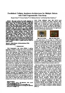
Quadrotor Control Architecture

For experimentation, we exploit the color characteristics of a simple target for detection and tracking. We used a combination of well established computer vision techniques to perform RGB normalization, color segmentation and blob detection. In this way, we consistently extracted only the color associated with the target. Its centroid was taken as the point feature and the spherical coordinates derived as per section III. B. Results Initially no assumptions were made on the roll and pitch velocity and they were included in the control. It was found that the control law was quite sensitive to inaccurate velocity measurements, causing the quad to issue more aggressive and rapidly fluctuating z velocity commands. Removing the optic flow measured from the IMU’s due to pitch and roll and adopting the control law derived in section III alleviated this problem. The effects of underestimating range were also validated. We present an instance similar to simulation in which the target was first detected to the right and below the quad rotor. The range used was set to 2m and the optic flow from vx was ignored. This is a difficult but realistic case, as we can no longer estimate the optic flow produced by the forward velocity and are not relying on range. The quad was allowed to fly toward the target at approximately 0.25ms−1 with heading around 0 degrees. When 4.5m away from the target, the visual control was activated. Figure 9 shows the trajectory of the quad and figure 10 shows the

φ

150 Colatitude (deg)

(

θ

100

50

0 −100

ψ 0

−50 −10

0 100 Azimuth (deg)

0

Feature Error

−10 σ γ

−30 0

5

10 Time (s)

20

Control

0

−20

10 Time (s)

10

Error (deg)



Fig. 8.

4

0

( )]



2 X (m)

VICON SPACE & IR CAMERAS

[

0

Target Range



QUAD ROTOR + IMU



-

6

8

( )]

( )

4 X (m)

Angle (deg)

∗

[



0

1

0 +

XY Position (Local Frame)

3

Velocity Control(ms−1)/(degs−1)

[

"

#$%& (

image feature error, control and orientation of the platform.

Range (m)

off board. A simple arrangment of PID controllers was used to control forward and lateral velocity whilst the vertical velocity and yaw rate were controlled directly using the derived IBVS scheme. The translational velocity was measured using a T40 Vicon and the body angles and rates from both Vicon and IMU. The true target range was obtained from the Vicon when required and a fixed value was used otherwise. To regulate the x and y velocity to a reference value, roll and pitch must be adjusted. Reference roll and pitch velocities were derived from x and y translational velocity measurements then compared to IMU measurements to derive the required feedback. The control architecture is depicted in figure 8.

15

5 0 −5

vz ωz

−10 −15 0

5

10

15

Time (s)

Fig. 10. Feature error, control & orientation for desired azimuth 25◦ and colatitude 80◦ . The black dashed lines show a 3 degree error margin.

Notice the feature error follows a similar pattern to figure 7 but the quad velocity has caused the stopping criteria to be met before the azimuth error has time to converge to zero. Having not accounted for optic flow from forward velocity, a smooth trajectory was still achieved but forced the controller to issue weaker z velocity commands and stronger ωz commands. The azimuth angle has gone past the desired position before attempting to settle with a positive offset error. From a collision avoidance standpoint this is not a problem as the more aggressive initial ωz control corresponds to an attempt to follow a larger spiral and thus allowed for an increased lateral separation at a faster rate. We notice a singularity occurs in the control if the target appears directly above or below the camera. Operating away

Fig. 11. Experimental Setup. Left:On board camera view. Centre:Lab view 1. Right: Lab View 2.

from this point, the effects were not observed during the large number of flight trials undertaken but need to be addressed. VI. CONCLUSIONS A method for reactive collision avoidance using single point targets based on conical spirals and spherical IBVS was presented. The approach can be adapted to other types of UAS and does not require an accurate estimate of range to avoid collision. Experimental results for a quad rotor platform were shown, providing some practical research on the Sense and Avoid problem under realistic problem constraints. This work is also believed to be the first practical implementation of a spherical image-based visual servoing scheme derived in [18]. Provided the Vicon is removed from the control loop, we could exploit the results in future work to estimate a probability of collision using the approach. This metric is often used to verify performance of deployable collision avoidance systems. Further work also includes analysis of the different control laws that would be derived by reorientating the camera axis with respect to the body frame and selecting different degrees of freedom to control. As such, a switched control scheme may be useful in order to ensure avoidance of any unstable regions on the sphere. Another approach may be to apply a control law that does not require defining a constant desired feature but instead moves the target around the sphere in such a way that any potential singularity problems are always avoided and a safe region of the sphere is reached. ACKNOWLEDGMENT The authors would like to thank Miguel A. OlivaresMendez and Ignacio Mellado-Bataller for their contributions to the experimental setup required for this study. R EFERENCES [1] K. Dalamagkidis, K. P. Valavanis, and L. A. Piegl, “On unmanned aircraft systems issues, challenges and operational restrictions preventing integration into the national airspace system,” Progress in Aerospace Sciences, 2008 vol. 44, no. 7-8, pp. 503–519. [2] F. Barfield, W. Res, D. Center, and A. F. B. Wright-Patterson, “Autonomous collision avoidance: the technical requirements,” in Proc. IEEE National Aerospace and Electronics Conf., NAECON’00, Oct. 2000, pp. 808–813.

[3] R. J. Kephart, “Comparison of see-and-avoid performance in manned and remotely piloted aircraft,” Ph.D. dissertation, Ohio University, 2008. [4] Australian Transport Safety Bureau (ATSB), “Limitations of the seeand-avoid principle,”Australian Government, Tech. Rep., November 2004. [5] J. Lai, L. Mejias, and J. Ford, “Airborne vision-based collisiondetection system,” Journal of Field Robotics, vol. 28, no. 2, pp. 137– 157, March 2011. [6] L. Mejias, J. Ford, and J. S. Lai, “Towards the implementation of vision-based uas sense-and-avoid,” in Proc. 27th Int. Congress of the Aeronautical Sciences, Sep. 2010. [7] B. R. Fajen and W. H. Warren, “Behavioral dynamics of steering, obstacle avoidance, and route selection,” Journal of Experimental Psychology-Human Perception and Performance, vol. 29, no. 2, pp. 343–361, 2003. [8] J. Kuchar and L. C. Yang, “Survey of conflict detection and resolution modeling methods,” IEEE Trans. Intelligent Transportation Systems, vol. 1, no. 4, pp. 179–189, Dec. 2000. [9] S. Hutchinson, G. D. Hager, and P. I. Corke, “A tutorial on visual servo control,” IEEE Trans. Robotics and Automation, vol. 12, no. 5, pp. 651–670, Oct. 1996. [10] S. C. L. Scherer, S. Singh, “Flying fast an low among obstacles: methodology and experiments,” The Int. Journal of Robotics Research, vol. 27, no. 5, pp. 549–574, May 2008. [11] S. Hrabar, G. S. Sukhatme, P. Corke, K. Usher, and J. Roberts, “Combined optic-flow and stereo-based navigation of urban canyons for a uav,” in Proc. IEEE/RSJ Int. Conf. Intelligent Robots and Systems, IROS’05, Oct. 2005, pp. 3309–3316. [12] S. Hrabar,“3D path planning and stereo-based obstacle avoidance for rotorcraft UAVs,” in Proc. IEEE/RSJ Int. Conf. Intelligent Robots and Systems, IROS’08, Sept. 2008, pp. 807–814 [13] T. Hamel and R. Mahony, “Image based visual servo control for a class of aerial robotic systems,” Automatica, vol. 43, no. 11, pp. 1975–1983, Nov. 2007. [14] O. Bourquardez, R. Mahony, N. Guenard, F. Chaumette, T. Hamel, and L. Eck, “Image-based visual servo control of the translation kinematics of a quadrotor aerial vehicle,” IEEE Trans. Robotics, vol. 25, no. 3, pp. 743–749, June 2009. [15] C. Teuliere, L. Eck, E. Marchand, and N. Guenard, “3d modelbased tracking for uav position control,” in Proc. IEEE/RSJ Int. Conf. Intelligent Robots and Systems, IROS’10, Oct. 2010, pp. 1084–1089. [16] P. I. Corke, F. Spindler, and F. Chaumette, “Combining cartesian and polar coordinates in ibvs,” in Proc. IEEE/RSJ Int. Conf. Intelligent Robots and Systems, IROS’09, Oct. 2009, pp. 5962–5967. [17] R. T. Fomena, O. Tahri, and F. Chaumette, “Visual servoing from three points using a spherical projection model,” in Proc. IEEE Int. Conf. Robotics and Automation, ICRA’10, Sep. 2010, pp. 5537–5542. [18] P. I. Corke, “Spherical image-based visual servo and structure estimation,” in Proc. IEEE Int. Conf. Robotics and Automation, ICRA’10, Sep. 2010, pp. 5550–5555. [19] W. Green, P.-Y. Oh,“Optic-flow-based collision avoidance,” IEEE Robotics & Automation Magazine, vol. 15, no. 1, pp. 93–106, March 2008. [20] A. Beyeler, J.-C. Zufferey, and D. Floreano, “Vision-based control of near-obstacle flight,” Autonomous Robots, vol. 27, pp. 201–219, July 2009. [21] J. Saunders and R. Beard, “Reactive vision based obstacle avoidance with camera field of view constraints,” in AIAA Guidance, Navigation and Control Conf. and Exhibit 2008. [22] R. Sharma, J. Saunders, and R. Beard, “Reactive path planning for micro air vehicles using bearing only measurements,” Journal of Intelligent Robotic Systems, vol. 65, pp. 409–416, Jan. 2012. [23] A. D. Mcfadyen and L. Mejias, “Visual servoing approach to collision avoidance for aircraft,” in Proc. 28th Int. Congress of the Aeronautical Sciences, ICAS’12, Sep. 2012. [24] W. Maddern and G. Wyeth, “Development of a hemispherical compound eye for egomotion estimation,” in Australasian Conf. Robotics and Automation, ACRA’08, Dec. 2008. [25] C. Geyer and K. Daniilidis, “A unifying theory for central panoramic systems and practical implications,” in Proc. 6th European Conf. Computer Vision, ECCV’08, June 2000 [26] K. N. Boyadzhiev, “Spirals and conchospirals in flight of insects,” The College Mathematics Journal, vol. 30, pp.23-31, Jan. 1999.