Abstract. Case Based Reasoning systems are often faced with the prob- ... Case-Based Reasoning (CBR) systems solve problems by reusing the solutions to.
Rough Sets Reduction Techniques for Case-Based Reasoning Maria Salam´ o and Elisabet Golobardes Enginyeria i Arquitectura La Salle, Universitat Ramon Llull, Psg. Bonanova 8, 08022 Barcelona, Spain {mariasal,elisabet}@salleurl.edu
Abstract. Case Based Reasoning systems are often faced with the problem of deciding which instances should be stored in the case base. An accurate selection of the best cases could avoid the system being sensitive to noise, having a large memory storage requirements and, having a slow execution speed. This paper proposes two reduction techniques based on Rough Sets theory: Accuracy Rough Sets Case Memory (AccurCM) and Class Rough Sets Case Memory (ClassCM). Both techniques reduce the case base by analysing the representativity of each case of the initial case base and applying a different policy to select the best set of cases. The first one extracts the degree of completeness of our knowledge. The second one obtains the quality of approximation of each case. Experiments using different domains, most of them from the UCI repository, show that the reduction techniques maintain accuracy obtained when not using them. The results obtained are compared with those obtained using well-known reduction techniques.
1
Introduction and Motivation
Case-Based Reasoning (CBR) systems solve problems by reusing the solutions to similar problems stored as cases in a case memory [19] (also known as case-base). However, these systems are sensitive to the cases present in the case memory and often its good accuracy rate depends on the significant cases stored. Therefore, in CBR systems it is important to reduce the case memory in order to remove noisy cases. This reduction allows us to achieve a good generalisation accuracy. In this paper we present an initial approach to two different reduction techniques based on Rough Sets theory. Both reduction techniques was introduced into our Case-Based Classifier System called BASTIAN. Case-Based Reasoning and Rough Sets theory have usually been used separately in the literature. The first one, Case-Based Reasoning [19,10], is used in a wide variety of fields and applications (e.g. diagnosis, planning, language understanding). We use Case-Based Reasoning as an automatic classification system. On the other hand, Rough Sets theory [16] is a Data Mining technique. The main research trends in Rough Sets theory -which tries to extend the capabilities of reasoning systems- are: (1) the treatment of incomplete knowledge; (2) the management of inconsistent pieces of information; and (3) the manipulation of D.W. Aha and I. Watson (Eds.): ICCBR 2001, LNAI 2080, pp. 467–482, 2001. c Springer-Verlag Berlin Heidelberg 2001
468
M. Salam´ o and E. Golobardes
various levels of representation, moving from refined universes of discourse to coarser ones and conversely. The reduction techniques proposed are: Accuracy Rough Sets Case Memory (AccurCM) and Class Rough Sets Case Memory (ClassCM). Both Rough Sets reduction techniques use the reduction of various levels of information. From those levels of information we extract relevant cases. The first technique, AccurCM, extracts an accuracy measure to capture the degree of completeness of our knowledge. The second one, ClassCM, obtains the quality of approximation of each case. It expresses the percentage of possible correct decisions when the case classifies new cases. The paper is structured as follows: section 2 introduces related work; next, section 3 explains the Rough Sets theory; section 4 details the proposed Rough Sets reduction techniques; section 5 describes the Case-Based Classifier System used in this study; section 6 exposes the testbed of the experiments and the results obtained; and finally, section 7 presents the conclusions and further work.
2
Related Work
Case-Based Reasoning systems solve problems by reusing a corpus of previous solving experience stored (set of training instances or cases T ) as a case memory of solved cases t. Reduction techniques are applied in Case-Based Reasoning systems for two main reasons: (1) to reduce storage requirements by increasing execution speed, and (2) to avoid sensitivity to noise. Thus, a performance goal for any CBR system is the maintenance of a case memory T maximizing coverage and minimizing case memory storage requirements. Reduction techniques remove instances of T obtaining a new training set S, S ⊆ T , that aims to maintain the generalization performance as well as reduce the storage requirements. Many researchers have addressed the problem of case memory reduction [26]. Related work on pruning a set of cases comes from the pattern recognition and machine learning community, most of them through studies of nearest neighbour algorithm (NNA), and Instance-Based Learning (IBL) methods. The first kind of approaches to the reduction of the case memory are commonly known as nearest neighbours editing rules. Most algorithms look for a subset of cases S of the original case memory T . The first approach was Condensed Nearest Neighbour (CNN) [9], which ensures that all cases in T are classified correctly, though it does not guarantee a minimal set and it is sensitive to noise. Selective Nearest Neighbour (SNN) [20] extends CNN such that every member of T must be closer to a member of S of the same class than to any member of T (instead of S) of a different class. SNN is more complex than other reduction techniques and its learning time is significantly greater; it is also sensitive to noise. Reduced Nearest Neighbour (RENN) [6] removes an instance from S if any other instance in T is misclassified by the instances remaining in S. RENN is computationally more expensive than CNN, but it is able to remove noisy instances while retaining border cases (i.e. cases that are placed at the boundaries of two classes). Edited Nearest Neighbour rule (ENN)[26], removes noisy
Rough Sets Reduction Techniques for Case-Based Reasoning
469
instances, and maintains internal cases and close border ones. Variable Similarity Metric (VSM)[13], removes instances depending on a confidence level and all the K nearest neighbours. VSM is able to remove noisy instances and internal instances and retains border ones. The second kind of approaches are related to Instance Based Learning Algorithms (IBL) [1]. IB1 is a simple implementation of NNA. IB2 is an incremental algorithm that does not necessarily classify all the instances correctly because it is sensitive to noise. IB2 is similar to CNN; it retains border points while it eliminates cases that are surrounded by members of the same class. IB3 improves IB2 retaining only those cases that have acceptable bounds. IB3 produces higher reduction than IB2 and higher accuracy. It also reduces sensitivity to noise. IB4 extends IB3, by building a set of attribute weights for each class. There is another way to approach this problem. There are systems that modify the instances themselves, instead of simply deciding which ones to keep. RISE [3] treats each instance as a rule that can be generalised. EACH [23] introduced the Nested Generalized Exemplars (NGE) theory, in which hyperrectangles are used to replace one or more instances, thus reducing the original training set. Another approach to instance pruning systems are those that take into account the order in which instances are removed [26]. DROP1 is similar to RNN and RISE, with some differences. DROP1 removes an instance from S (where S = T originally) if at least as many of its associates in S would be classified correctly without it. This heuristic has some problems with noisy instances, which DROP2 tries to solve by removing an instance from S if at least as many of its associates in T would be classified correctly without it. DROP3 is designed to filter noise before sorting the instances. DROP4 is a more careful noise filter. Finally, DROP5 modifies DROP2 trying to smooth the decision boundary. Finally, researchers have also focused on increasing the overall competence, the range of target problems that can be successfully solved, of the case memory through case deletion [24]. Strategies have been developed for controlling case memory growth through methods such as competence-preserving deletion [24] and failure-driven deletion [18], as well as for generating compact case memories through competence-based case addition [25,28]. Leake and Wilson [11] examine the benefits of using fine-grained performance metrics to directly guide case addition or deletion. This method is specially important for task domains with non-uniform problem distributions. Finally, a case-base maintenance method that avoids building sophisticated structures around a case-base or complex operations is presented by Yang and Wu [27]. Their method partitions cases into clusters where the cases in the same cluster are more similar than cases in other clusters. Clusters can be converted to new smaller case-bases.
3
Rough Sets Theory
Zdzislaw Pawlak introduced Rough Sets theory in 1982 [16,17]. The idea of Rough Sets consists of the approximation of a set by a pair of sets, called the lower and the upper approximation of this set. In fact, these approximations
470
M. Salam´ o and E. Golobardes
are inner and closure operations in a certain topology. These approximations are generated by the available data about the elements of the set. The nature of Rough Sets theory makes them useful for reducing knowledge, extracting dependencies in knowledge, reasoning about knowledge, pattern recognition, etc. We use Rough Sets theory for reducing and extracting the dependencies in knowledge. This reduction of knowledge is the basis for computing the relevance of instances into the Case-Based Classifier System. We use that relevance in two different ways. The first one is Accuracy Rough Sets Case Memory and the second one is Class Rough Sets Case Memory. First of all, we incorporate some concepts and definitions. Then, we explain how to obtain the dependencies, in order to select the set of instances. Basic Concepts and Definitions We have a Universe (U ) (finite not null set of objects that describes our problem, i.e. the case memory). We compute from our universe the concepts (objects or cases) that form partitions. The union of all the concepts make the entire Universe. Using all the concepts we can describe all the equivalence relations (R) over the universe U . Let an equivalence relation be a set of features that describe a specific concept. U/R is the family of all equivalence classes of R. The universe and the relations form the knowledge base (K), defined as ˆ >. Where R ˆ is the family of equivalence relations over U . Every K =< U, R relation over the universe is an elementary concept in the knowledge base. All the concepts are formed by a set of equivalence relations that describe them. Thus, we search for the minimal set of equivalence relations that defines the same concept as the initial set. DefinitionT1 (Indiscernibility Relations) ˆ where Pˆ ⊆ R. ˆ The indiscernibility relation is an equivalence relation IN D(Pˆ ) = R over U . Hence, it partitions the concepts (cases) into equivalence classes. These sets of classes are sets of instances indiscernible with respect to the features in P . Such a partition is denoted as U/IN D(P ). In supervised machine learning, the sets of cases indiscernible with respect to the class attribute contain the cases of each class.
4
Rough Sets as Reduction Techniques
In this section we explain how to reduce the case memory using the Rough Sets theory. We obtain a minimal case memory unifying two concepts: (1) approximation sets of knowledge and (2) reduction of search space. These two concepts are the basis for the AccurCM and ClassCM reduction techniques. Both reduction techniques deal with cases containing continuous, nominal and missing features. Rough Sets reduction techniques perform search approximating sets by other sets and both proposals are global. Global means that we select the representative knowledge without taking into account which class the cases classify. AccurCM computes an accuracy measure. ClassCM computes the
Rough Sets Reduction Techniques for Case-Based Reasoning
471
classification accuracy measure of each case in the representative knowledge. We want to remark that AccurCM and ClassCM can be used in multiclass tasks. First of all, this section explains how to approximate and reduce knowledge. Next, it describes the unification of both concepts to extract the reduced set of cases using two policies: (1) Accuracy Rough Sets Case Memory (AccurCM), and Class Rough Sets Case Memory (ClassCM). 4.1
Approximating and Reducing the Knowledge
Approximations of Set. This is the main idea of Rough Sets, to approximate a set by other sets. The condition set contains all cases present in the case memory. The decision set presents all the classes that the condition set has to classify. We are searching for a subset of the condition set able to classify the same as the initial set, so it approximates the same decision set. The following definitions explain this idea. ˆ > be a knowledge base. For any subset of cases X ⊆ U and an Let K =< U, R equivalence relation R ⊆ IN D(K) we associate two subsets called: Lower RX; and Upper RX approximations. If RX=RX then X is an exact set (definable using subset R), otherwise X is a rough set with respect to R. Definition 2 (Lower approximation) S The lower approximation, defined as: RX = {Y ∈ U/R : Y ⊆ X} is the set of all elements of U which can certainly be classified as elements of X in knowledge R. Definition 3 (Upper approximation) S T 6 ∅} is the set of elements The upper approximation, RX = {Y ∈ U/R : X Y = of U which can possibly be classified as elements of X, employing knowledge R. Example 1 If we consider a set of 8 objects in our Universe, U = {x1 , x2 , x3 , x4 , x5 , x6 , x7 , x8 }, ˆ = (A, B, C, D) as a family of equivalence relations over U . Where A = using R {x1 , x4 , x8 }, B = {x2 , x5 , x7 }, C = {x3 } and D = {x6 }. And we also consider 3 subsets of knowledge X1 , X2 , X3 . Where X1 = {x1 , x4 , x5 }, X2 = {x3 , x5 }, X3 = {x3 , x6 , x8 }. The lower and upper approximations are: S B = S{x1 , x2 , x4 , x5 , x7 , x8 } RX1 = ∅ and RX1 = A = {x3 } and RX2 = B C =S{x2 , S x3 , x5 , x7 } RX2 = C S RX3 = C D = {x3 , x6 } and RX3 = A C D = {x1 , x3 , x4 , x6 , x8 } Reduct and Core of knowledge. This part is related to the concept of reduction of the search space. We are looking for a reduction in the feature search space that defines the initial knowledge base. Next, reduction techniques apply this new space to extract the set of cases that represents the new case memory.
472
M. Salam´ o and E. Golobardes
Intuitively, a reduct of knowledge is its essential part, which suffices to define all concepts occurring in the considered knowledge, whereas the core is the most important part of the knowledge. ˆ be a family of equivalence relations and R ∈ R. ˆ We will say that: Let R ˆ 6= IN D(R ˆ − {R}); otherwise it is dispensable. – R is indispensable if IN D(R) ˆ − {R}) is the family of equivalence R ˆ extracting R. IN D(R ˆ is independent if each R ∈ R ˆ is indispensable in R; otherwise – The family R it is dependent. Definition 4 (Reduct) ˆ∈R ˆ is a reduct of R ˆ if : Q ˆ is independent and IN D(Q) ˆ = IN D(R). ˆ Obviously, Q ˆ may have many reducts. Using Q ˆ it is possible to approximate the same as using R ˆ R. Each reduct has the property that a feature can not be removed from it without changing the indiscernibility relation. Definition 5 (Core) ˆ will be called the core of R, ˆ and will be The set of all indispensable relations in R T ˆ = RED(R). ˆ Where RED(R) ˆ is the family of all reducts denoted as:CORE(R) ˆ The core can be interpreted as the set of the most characteristic part of of R. knowledge, which can not be eliminated when reducing the knowledge. Example 2 If we consider a set of 8 objects in our Universe, U = {x1 , x2 , x3 , x4 , x5 , x6 , x7 , x8 }, ˆ = {P, Q, S} as a family of equivalence relations over U . Where P can be using R colours (green, blue, red, yellow); Q can be sizes (small, large, medium); and S can be shapes (square, round, triangular, rectangular). For example, we can suppose that the equivalence classes are: U/P = { (x1 , x4 , x5 ), (x2 , x8 ), (x3 ),(x6 , x7 ) } U/Q ={ (x1 , x3 , x5 ), (x6 ), (x2 , x4 , x7 , x8 ) } U/S = { (x1 , x5 ), (x6 ), (x2 , x7 , x8 ), (x3 , x4 ) } As can be seen, every equivalence class divides the Universe in a different way. Thus the relation IN D(R) has the following equivalence classes: ˆ = {(x1 , x5 ),(x2 , x8 ),(x3 ),(x4 ),(x6 ),(x7 )} U/IN D(R) ˆ since: The relation P is indispensable in R, ˆ ˆ U/IN D(R − {P }) = { (x1 , x5 ), (x2 , x7 , x8 ), (x3 ), (x4 ), (x6 ) } 6= U/IN D(R). ˆ The information obtained removing relation Q is equal, so it is dispensable in R. ˆ ˆ − {Q}) = { (x1 , x5 ), (x2 , x8 ), (x3 ), (x4 ), (x6 ), (x7 ) }=U/IN D(R). U/IN D(R Hence the relation S is also dispensable in R. ˆ ˆ − {S}) = { (x1 , x5 ), (x2 , x8 ), (x3 ),(x4 ), (x6 ), (x7 ) }=U/IN D(R). U/IN D(R That means that the classification defined by the set of three equivalence relations P, Q and S is the same as the classification defined by relation P and Q ˆ = {(P, Q), (P, S)} and or P and S. Thus, the reducts and the core are: RED(R) ˆ CORE(R) = {P }.
Rough Sets Reduction Techniques for Case-Based Reasoning
4.2
473
Reducing the Set of Cases
Accuracy Rough Sets Case Memory and Class Rough Sets Case Memory, the methods which we propose, use the information of reducts and core to select the cases that are maintained in the case memory. Accuracy Rough Sets Case Memory. This reduction technique computes the Accuracy reducts coefficient (AccurCM) of each case in the knowledge base (case memory). The coefficient µ(t) is computed as: F or each instance t ∈ T it computes : µ(t) =
card ( P (t)) card ( P (t))
(1)
Where µ(t) is the relevance of the instance t; P is the set that contains the reducts and core obtained from the original data; T is the condition set; card is the cardinality of one set; and finally P and P are the lower and upper approximations, respectively. For each case we apply the following algorithm, where the confidenceLevel is the µ(t) value computed: 1. Algorithm SelectCases 2. conf idenceLevel = 0.0 3. for each case 4. select the case if it accomplishes this confidenceLevel 5. end for 6. end Algorithm In this algorithm the conf idenceLevel is set at to zero, in order to only select the set of cases that accomplishes this space region. Inexactness of a set of cases is due to the existence of a borderline region. The greater a borderline region of a set, the lower the accuracy of the set. The accuracy measure expresses the degree of completeness of our knowledge about the set P . This reduction technique obtains the minimal set of instances present in the original case memory. The accuracy coefficient explains if an instance is needed or not, so µ(t) is a binary value. When the value µ(t)= 0 it means an internal case, and a µ(t) =1 means a borderline case. This technique does not guarantee that all classes will be present in the set of instances selected. However, it guarantees that all the internal points that represent a class will be included. The accuracy expresses the percentage of possible correct decisions when classifying cases employing knowledge P . This measure approximates the coverage of each case. Class Rough Sets Case Memory. In this reduction technique we use the quality of classification coefficient (ClassCM), computed using the core and reducts of information. The classification accuracy coefficient µ(t) is computed as: F or each instance t ∈ T it computes : µ(t) =
card ( P (t)) card ( all instances)
(2)
474
M. Salam´ o and E. Golobardes
Where µ(t) is the relevance of the instance t; P is the set that contains the reducts and core obtained from the original data; T is the condition set; card is the cardinality of one set; and finally P is the lower approximation. The ClassCM coefficient expresses the percentage of cases which can be correctly classified employing the knowledge t. This coefficient (µ(t)) has a range of values between 0 to 1, where 0 means that the instance classifies incorrectly the range of cases that belong to its class and a value of 1 means an instance that classifies correctly the range of cases that belong to its class. In this reduction technique the cases that obtain a higher value of µ(t) represent cases that classify correctly the cases, but these cases are to be found on the search space boundaries. This reduction technique guarantees a minimal set of instances of each class also applying the following algorithm, where the confidenceLevel is the µ(t) computed previously: 1. Algorithm SelectCases 2. conf idenceLevel = 1.0 and f reeLevel = ConstantT uned (set at 0.01) 3. select all possible cases that accomplish this confidenceLevel 4. while all classes are not selected 5. confidenceLevel = confidenceLevel - freeLevel 6. select all possible cases that accomplish this confidenceLevel 7. end while 8. end Algorithm Due to the range of values, it is possible to select not only the best set of instances as ClassCM computes. We select a set of instances depending on the confidence level of µ(t) that we compute. The confidence level is reduced until all the classes have a minimum of one instance present in the new case memory. The introduction of these techniques into a CBR system is explained in section 5.1.
5
Description of the BASTIAN System
The study described in this paper was carried out in the context of BASTIAN, a case-BAsed SysTem In clAssificatioN [22,21]. This section details two points: (1) the main capabilities of the BASTIAN platform used in the study carried out in this paper, in order to understand what kind of CBR cycle has been applied in the experimental analysis; (2) how to introduce the Rough Sets reduction techniques into a Case-Based Reasoning System. The BASTIAN system is an extension of CaB-CS (Case-Based Classifier System) system [5]. The BASTIAN system allows the user to test several variants of CBR (e.g. different retrieval or retain phases, different similarity functions and weighting methods). For details related to the BASTIAN platform see [22]. BASTIAN has been developed in JAVA language and the system is being improved with new capabilities.
Rough Sets Reduction Techniques for Case-Based Reasoning
475
BASTIAN Platform Capabilities The system capabilities are developed to work separately and independently in co-operation with the rest. Each capability described in the general structure has a description of the general behaviour that it has to achieve. The main goal is to obtain a general structure that could change dynamically depending on the type of Case-Based Reasoner we want to develop. The main capabilities are: – The CaseMemory defines the behaviour for different case memory organizations. In this study, we use a list of cases. Our main goal in this paper is to reduce the case memory; for this reason, we have not focus on the representation used by the system. – The SimilarityFunctionInterface concentrates on all the characteristics related to similarity functions. It allows us to change the similarity function dynamically within the system. In this paper, we use the K-Nearest Neighbour similarity function. – The WeightingInterface contains the main abilities to compute the feature relevance in a Case-Based Classifier System [22]. It is related to the RetrievalInterface and the SimilarityFunctionInterface. This paper does not use them in order to test the reliability of our new reduction techniques. Further work will consist of testing the union of both proposals. – The {Retrieval, Reuse, Revise, Retain}Interface are the four phases of the CBR cycle. These interfaces describe the behaviour of each phase. • Retrieval interface is applied using K=1 and K=3 values in the K-NN policy. • {Reuse, Revise, Retain} interface are applied choosing a standard configuration for the system, in order to analyse only the reduction techniques. Our aim, is to improve the generalisation accuracy of our system by reducing the case memory in order to remove the noisy instances and maintain border points [26]. 5.1
Rough Sets Inside the BASTIAN Platform
Figure 1 shows the meta-level process when incorporating the Rough Sets into the CBR system. The Rough Sets process is divided into three steps: The first one discretises the instances, it is necessary to find the most relevant information using the Rough Sets theory. In that case, we discretise continuous features using [4] algorithm. The second step searches for the reducts and the core of knowledge using the Rough Sets theory, as was described in section 4. Finally, the third step uses the core and the reducts of knowledge to decide which cases are maintained in the case memory using AccurCM and ClassCM techniques, as explained in 4.2. Rough Sets theory has been introduced as reduction techniques in two phases of the CBR cycle. The first phase is the start-up phase and the second one is the retain phase. The system adds a previous phase Startup, which is not in the Case-Based Reasoning cycle.
476
M. Salam´ o and E. Golobardes
This initial phase prepares the initial start-up of the system. It computes the new initial case memory from the training case memory; this new case memory is used by the retrieval phase later. The retain phase computes a new case memory from the case memory if a new case is stored. In this paper, we focus our reduction techniques on the retrieval phase. The code of Rough Sets theory in the Case-Based Reasoning has been implemented using a public Rough Sets Library [7]. Set of Instances
Set of instances
Discretise
BASTIAN
Searching REDUCTS & CORE
Rough Sets
Instances Extraction
BASTIAN
Fig. 1. High level process of Rough Sets.
6
Empirical Study
This section is structured as follows: first, we describe the testbed used in the empirical study; then we discuss the results obtained from the reduction techniques based on Rough Sets. We compare the results compared to CBR system working with the original case memory. And finally, we also compare the results with some related learning systems. 6.1
Testbed
In order to evaluate the performance rate, we use twelve datasets. Datasets can be grouped in two ways: public and private. The datasets and their characteristics are listed in table 1. Public datasets are obtained from the UCI repository [15]. They are: breast cancer Wisconsin (breast-w), glass, ionosphere, iris, sonar and vehicle. Private datasets comes from our own repository. They deal with diagnosis of breast cancer and synthetic datasets. Datasets related to diagnosis are biopsy and mammogram. Biopsy [5] is the result of digitally processed biopsy images, whereas mammogram consists of detecting breast cancer using the microcalcifications present in a mammogram [14,8]. In mammogram each example contains the description of several µCa present in the image; in other words, the input information used is a set of real valued matrices. On the other hand, we use two synthetic datasets to tune up the learning algorithms, because we knew their solutions in advance. MX11 is the eleven input multiplexer. TAO-grid is a dataset obtained from sampling the TAO figure using a grid [12].
Rough Sets Reduction Techniques for Case-Based Reasoning
477
These datasets were chosen in order to provide a wide variety of application areas, sizes, combinations of feature types, and difficulty as measured by the accuracy achieved on them by current algorithms. The choice was also made with the goal of having enough data points to extract conclusions. All systems were run using the same parameters for all datasets. The percentage of correct classifications has been averaged over stratified ten-fold crossvalidation runs, with their corresponding standard deviations. To study the performance we use paired t-test on these runs. Table 1. Datasets and their characteristics used in the empirical study. Dataset 1 2 3 4 5 6 7 8 9 10
6.2
Biopsy Breast-w Glass Ionosphere Iris Mammogram MX11 Sonar TAO-Grid Vehicle
Refe Sam- NumeSimbo- Cla- Inconrence ples ric feats. lic feats. sses sistent BI BC GL IO IR MA MX SO TG VE
1027 699 214 351 150 216 2048 208 1888 846
24 9 9 34 4 23 60 2 18
11 -
2 2 6 2 3 2 2 2 2 4
Yes Yes No No No Yes No No No No
Experimental Analysis of Reduction Techniques
Table 2 shows the experimental results for each dataset using CBR system Rough Sets reduction techniques: AccurCM and ClassCM, IB2, IB3 and IB4 [1]. This table contains the mean percentage of correct classifications (%PA)(competenceof the system) and the mean storage size (%MC). We want to compare the results obtained using the proposed ClassCM reduction technique with those obtained by these classifier systems. Time performance is beyond the scope of this paper. Both Rough Sets reduction techniques have the same initial concept: to use the reduction of knowledge to measure the accuracy (AccurCM) or the quality of classification (ClassCM). Although reduction is important, we decided to use these two different policies in order to maintain or even improve, if possible, prediction accuracy when classifying a new case. That fact is detected in the results. For example, the vehicle dataset obtains good accuracy as well as reduces the case memory, in both techniques. However, the case memory reduction is not large. There are some datasets that obtain a higher reduction of the case memory but decrease the prediction accuracy, although this reduction in not significant.
478
M. Salam´ o and E. Golobardes
Table 2. Mean percentage of correct classifications and mean storage size. Two-sided paired t-test (p = 0.1) is performed, where a • and ◦ stand for a significant improvement or degradation of our ClassCM approach related to the system compared. Bold font indicates the best prediction accuracy. Ref.
CBR %PA %CM BI 83.15 100.0 BC 96.28 100.0 GL 72.42 100.0 IO 90.59 100.0 IR 96.0 100.0 MA 64.81 100.0 MX 78.61 100.0 SO 84.61 100.0 TG 95.76 100.0 VE 67.37 100.0
AccurCM %PA %CM 75.15• 2.75 94.56 58.76 58.60• 23.88 88.60• 38.98 94.00◦ 96.50 66.34◦ 81.56 68.00• 0.54 75.48• 33.01 96.34◦ 95.39 64.18• 34.75
ClassCM %PA %CM 84.41 1.73 96.42 43.95 71.12 76.11 92.59 61.00 87.40 8.85 59.34 37.50 78.74 99.90 86.05 67.05 86.97 13.14 68.42 65.23
IB2 %PA %CM 75.77• 26.65 91.86• 8.18 62.53• 42.99 86.61• 15.82 93.98◦ 9.85 66.19 42.28 87.07◦ 18.99 80.72 27.30 94.87◦ 7.38 65.46• 40.01
IB3 %PA %CM 78.51• 13.62 94.98 2.86 65.56• 44.34 90.62 13.89 91.33 11.26 60.16 14.30 81.59 15.76 62.11• 22.70 95.04◦ 5.63 63.21• 33.36
IB4 %PA %CM 76.46• 12.82 94.86 2.65 66.40• 39.40 90.35 15.44 96.66 12.00 60.03 21.55 81.34 15.84 63.06• 22.92 93.96◦ 5.79 63.68• 31.66
Comparing AccurCM and ClassCM, the most regular behaviour is achieved using ClassCM. This behaviour is due to its own nature, because it introduces all the border cases classifying the class correctly into the reduced case memory, as well as the internal cases needed to complete all classes. AccurCM calculates the border points of the case memory. AccurCM calculates the degree of completeness of our knowledge, which can be seen as the coverage [25]. AccurCM points out the relevance of classification of each case. ClassMC reduction technique obtains on average a higher generalisation accuracy than IBL, as can be seen in table 2. There are some datasets where ClassCM shows a significant increase in the prediction accuracy. The performance of IBL algorithms declines when case memory is reduced. CBR obtains on average higher prediction accuracy than IB2, IB3 and IB4. On the other hand, the mean storage size obtained for ClassCM is higher than that obtained when using IBL schemes (see table 2). IBL algorithms obtain a higher reduction of the case memory. However, IBL performance declines, in almost all datasets (e.g. Breast-w, Biopsy). This degradation is significant in some datasets, as happens with the sonar dataset. Our initial purpose for the reduction techniques was to reduce the case memory as much as possible, maintaining the generalisation accuracy. We should continue working to obtain a higher reduction on the case memory. To finish the empirical study, we also run additional well-known reduction schemes on the previous data sets. The reduction algorithms are: CNN, SNN, DEL, ENN, RENN, DROP1, DROP2, DROP3, DROP4 and DROP5 (a complete explanation of them can be found in [26]). We use the same data sets described above but with different ten-fold cross validation sets. We want to compare the results obtained using the proposed ClassCM reduction technique with those obtained by these reduction techniques. Tables 3 and 4 show the mean prediction accuracy and the mean storage size for all systems in all datasets, respectively. Table 3 shows the behaviour of our ClassCM reduction technique in comparison with CNN, SNN, DEL, ENN and RENN techniques. The results are on average better than those obtained by the reduction techniques studied. RENN
Rough Sets Reduction Techniques for Case-Based Reasoning
479
Table 3. Mean percentage of correct classifications and mean storage size. Two-sided paired t-test (p = 0.1) is performed, where a • and ◦ stand for a significant improvement or degradation of our ClassCM approach related to the system compared. Bold font indicates the best prediction accuracy. Ref.
ClassCM %PA %CM BI 84.41 1.73 BC 96.42 43.95 GL 71.12 76.11 IO 92.59 61.00 IR 87.40 8.85 MA 59.34 37.50 MX 78.74 99.90 SO 86.05 67.05 TG 86.97 13.14 VE 68.42 65.23
CNN %PA %CM 79.57• 17.82 95.57 5.87 67.64 24.97 88.89• 9.94 96.00◦ 14.00 61.04 25.06 89.01◦ 37.17 83.26 23.45 94.39◦ 7.15 69.74 23.30
SNN %PA %CM 78.41• 14.51 95.42 3.72 67.73 20.51 85.75• 7.00 94.00◦ 9.93 63.42◦ 18.05 89.01◦ 37.15 80.38 20.52 94.76◦ 6.38 69.27 19.90
DEL %PA %CM 82.79• 0.35 96.57◦ 0.32 64.87• 4.47 80.34• 1.01 96.00◦ 2.52 62.53◦ 1.03 68.99• 0.55 77.45• 1.12 87.66 0.26 62.29• 2.55
ENN %PA %CM 77.82• 16.52 95.28 3.61 68.23 19.32 88.31• 7.79 91.33 8.59 63.85◦ 21.66 85.05◦ 32.54 85.62 19.34 96.77◦ 3.75 66.91 20.70
RENN %PA %CM 81.03• 84.51 97.00◦ 96.34 68.66 72.90 85.18• 86.39 96.00◦ 94.44 65.32◦ 66.92 99.80◦ 99.89 82.74 86.49 95.18◦ 96.51 68.67 74.56
improves the results of ClassCM in some data sets (e.g. Breast-w ) but its reduction on the case memory is lower than ClassCM. Table 4. Mean percentage of correct classifications and mean storage size. Two-sided paired t-test (p = 0.1) is performed, where a • and ◦ stand for a significant improvement or degradation of our ClassCM approach related to the system compared. Bold font indicates best prediction accuracy. Ref.
ClassCM %PA %CM BI 84.41 1.73 BC 96.42 43.95 GL 71.12 76.11 IO 92.59 61.00 IR 87.40 8.85 MA 59.34 37.50 MX 78.74 99.90 SO 86.05 67.05 TG 86.97 13.14 VE 68.42 65.23
DROP1 %PA %CM 76.36• 26.84 93.28 8.79 66.39 40.86 81.20• 23.04 91.33 12.44 61.60 42.69 87.94◦ 19.02 84.64 25.05 94.76◦ 8.03 64.66• 38.69
DROP2 %PA %CM 76.95• 29.38 92.56 8.35 69.57 42.94 87.73• 19.21 90.00 14.07 58.33 51.34 100.00◦ 98.37 87.07 28.26 95.23◦ 8.95 67.16 43.21
DROP3 %PA %CM 77.34• 15.16 96.28 2.70 67.27 33.28 88.89 14.24 92.66 12.07 58.51 12.60 82.37 17.10 76.57• 16.93 94.49◦ 6.76 66.21 29.42
DROP4 %PA %CM 76.16• 28.11 95.00 4.37 69.18 43.30 88.02• 15.83 88.67 7.93 58.29 50.77 86.52 25.47 84.64 26.82 89.41◦ 2.18 68.21 43.85
DROP5 %PA %CM 76.17• 27.03 93.28 8.79 65.02• 40.65 81.20• 23.04 91.33 12.44 61.60 42.64 86.52 18.89 84.64 25.11 94.76◦ 8.03 64.66• 38.69
In table 4 the results obtained using ClassCM and DROP algorithms are compared. ClassCM shows better competence for some data sets (e.g. biopsy, breast-w, glass), although its results are also worse in others (e.g. multiplexer ). The behaviour of these reduction techniques are similar to the previously studied. ClassCM obtains a balance behaviour between competence and size. There are some reduction techniques that obtain best competence for some data sets reducing less the case memory size. All the experiments (tables 2, 3 and 4) point to some interesting observations. First, it is worth noting that the individual AccurCM and ClassCM works well in all data sets, obtaining better results on ClassCM because the reduction is smaller. Second, the mean storage obtained using AccurCM and ClassCM suggest complementary behaviour. This effect can be seen on the tao-grid data
480
M. Salam´ o and E. Golobardes
set, where AccurCM obtains a 95.39% mean storage and ClassCM 13.14%. We want to remember that ClassCM complete the case memory in order to obtain at least one case of each class. This complementary behaviour suggests that they can be used together in order to improve the competence and maximise the reduction of the case memory. Finally, the results on all tables suggest that all the reduction techniques work well in some, but not all, domains. This has been termed the selective superiority problem [2]. Consequently, future work consists of combining both approaches in order to exploit the strength of each one.
7
Conclusions and Further Work
This paper introduces two new reduction techniques based on the Rough Sets theory. Both reduction techniques have a different nature: AccurCM reduces the case memory maintaining the internal cases; and ClassCM obtains a reduced set of border cases, increasing that set of cases with the most relevant classifier cases. Empirical studies show that these reduction techniques produce a higher or equal generalisation accuracy on classification tasks. We conclude that Rough Sets reduction techniques should be improved in some ways. That fact focus our further work. First, the algorithm selectCases should be changed in order to select a most reduced set of cases. In this way, we want to modifiy the algorithm selecting only the most representative K-nearest neighbour cases that accomplishing the conf idenceLevel. Second, we should search for new discretisation methods in order to improve the pre-processing of the data. Finally, we want to analyse the influence of the weighting methods in these reduction techniques. Acknowledgements. This work is supported by the Ministerio de Sanidad y Consumo, Instituto de Salud Carlos III, Fondo de Investigaci´ on Sanitaria of Spain, Grant No. 00/0033-02. The results of this study have been obtained using the equipment co-funded by the Direcci´ o de Recerca de la Generalitat de Catalunya (D.O.G.C 30/12/1997). We wish to thank Enginyeria i Arquitectura La Salle (Ramon Llull University) for their support of our Research Group in Intelligent Systems. We also wish to thank: D. Aha for providing the IBL code and D. Randall Wilson and Tony R. Martinez who provided the code of the other reduction techniques. Finally, we wish to thank the anonymous reviewers for their useful comments during the preparation of this paper.
References 1. D. Aha and D. Kibler. Instance-based learning algorithms. Machine Learning, Vol. 6, pages 37–66, 1991. 2. C.E. Brodley. Addressing the selective superiority problem: Automatic algorithm/model class selection. In Proceedings of the 10th International Conference on Machine Learning, pages 17–24, 1993. 3. P. Domingos. Context-sensitive feature selection for lazy learners. In AI Review, volume 11, pages 227–253, 1997.
Rough Sets Reduction Techniques for Case-Based Reasoning
481
4. U.M. Fayyad and K.B. Irani. Multi-interval discretization of continuous-valued attributes for classification learning. In 19th International Joint Conference on Artificial Intelligence, pages 1022–1027, 1993. 5. J.M. Garrell, E. Golobardes, E. Bernad´ o, and X. Llor` a. Automatic diagnosis with Genetic Algorithms and Case-Based Reasoning. Elsevier Science Ltd. ISSN 09541810, 13:367–362, 1999. 6. G.W. Gates. The reduced nearest neighbor rule. In IEEE Transactions on Information Theory, volume 18(3), pages 431–433, 1972. 7. M. Gawry’s and J. Sienkiewicz. Rough Set Library user’s Manual. Technical Report 00-665, Computer Science Institute, Warsaw University of Technology, 1993. 8. E. Golobardes, X. Llor` a, M. Salam´ o, and J. Mart´ı. Computer Aided Diagnosis with Case-Based Reasoning and Genetic Algorithms. Knowledge Based Systems (In Press), 2001. 9. P.E. Hart. The condensed nearest neighbour rule. IEEE Transactions on Information Theory, 14:515–516, 1968. 10. J. Kolodner. Case-Based Reasoning. Morgan Kaufmann Publishers, Inc., 1993. 11. D. Leake and D. Wilson. Remembering Why to Remember:Performance-Guided Case-Base Maintenance. In Proceedings of the Fifth European Workshop on CaseBased Reasoning, 2000. 12. X. Llor` a and J.M. Garrell. Inducing partially-defined instances with Evolutionary Algorithms. In Proceedings of the 18th International Conference on Machine Learning (To Appear), 2001. 13. D.G. Lowe. Similarity Metric Learning for a Variable-Kernel Classifier. In Neural Computation, volume 7(1), pages 72–85, 1995. 14. J. Mart´ı, J. Espa˜ nol, E. Golobardes, J. Freixenet, R. Garc´ıa, and M. Salam´ o. Classification of microcalcifications in digital mammograms using case-based reasonig. In International Workshop on digital Mammography, 2000. 15. C. J. Merz and P. M. Murphy. UCI Repository for Machine Learning Data-Bases [http://www.ics.uci.edu/∼mlearn/MLRepository.html]. Irvine, CA: University of California, Department of Information and Computer Science, 1998. 16. Z. Pawlak. Rough Sets. In International Journal of Information and Computer Science, volume 11, 1982. 17. Z. Pawlak. Rough Sets: Theoretical Aspects of Reasoning about Data. Kluwer Academic Publishers, 1991. 18. L. Portinale, P. Torasso, and P. Tavano. Speed-up, quality and competence in multi-modal reasoning. In Proceedings of the Third International Conference on Case-Based Reasoning, pages 303–317, 1999. 19. C.K. Riesbeck and R.C. Schank. Inside Case-Based Reasoning. Lawrence Erlbaum Associates, Hillsdale, NJ, US, 1989. 20. G.L. Ritter, H.B. Woodruff, S.R. Lowry, and T.L. Isenhour. An algorithm for a selective nearest neighbor decision rule. In IEEE Transactions on Information Theory, volume 21(6), pages 665–669, 1975. 21. M. Salam´ o and E. Golobardes. BASTIAN: Incorporating the Rough Sets theory into a Case-Based Classifier System. In III Congr´ es Catal` a d’Intel·lig`encia Artificial, pages 284–293, October 2000. 22. M. Salam´ o, E. Golobardes, D. Vernet, and M. Nieto. Weighting methods for a Case-Based Classifier System. In LEARNING’00, Madrid, Spain, 2000. IEEE. 23. S. Salzberg. A nearest hyperrectangle learning method. Machine Learning, 6:277– 309, 1991.
482
M. Salam´ o and E. Golobardes
24. B. Smyth and M. Keane. Remembering to forget: A competence-preserving case deletion policy for case-based reasoning systems. In Proceedings of the Thirteen International Joint Conference on Artificial Intelligence, pages 377–382, 1995. 25. B. Smyth and E. McKenna. Building compact competent case-bases. In Proceedings of the Third International Conference on Case-Based Reasoning, 1999. 26. D.R. Wilson and T.R. Martinez. Reduction techniques for Instance-Based Learning Algorithms. Machine Learning, 38, pages 257–286, 2000. 27. Q. Yang and J. Wu. Keep it Simple: A Case-Base Maintenance Policy Based on Clustering and Information Theory. In Proc. of the Canadian AI Conference, 2000. 28. J. Zhu and Q. Yang. Remembering to add: Competence-preserving case-addition policies for case base maintenance. In Proceedings of the Fifteenth International Joint Conference on Artificial Intelligence, 1999.