Roughness correction to the Casimir force beyond perturbation theory

epl draft

Roughness correction to the Casimir force beyond perturbation theory

arXiv:1106.4706v1 [cond-mat.mes-hall] 23 Jun 2011

Wijnand Broer1 , George Palasantzas1, Jasper Knoester1 , and Vitaly B. Svetovoy2 1

Zernike Institute for Advanced Materials, University of Groningen, Nijenborgh 4, 9747 AG Groningen, The Netherlands 2 MESA+ Institute for Nanotechnology, University of Twente, P.O. Box 217, 7500 AE Enschede, The Netherlands

PACS PACS PACS

03.70.+k – Theory of quantized fields 68.37.Ps – Atomic force microscopy (AFM) 85.85.+j – Micro- and nano-electromechanical systems (MEMS/NEMS) and devices

Abstract –Up to now there has been no reliable method to calculate the Casimir force when surface roughness becomes comparable with the separation between bodies. Statistical analysis of rough Au films demonstrates rare peaks with heights considerably larger than the root-meansquare (rms) roughness. These peaks define the minimal distance between rough surfaces and can be described with extreme value statistics. We show that the contributions of high peaks to the force can be calculated independently of each other while the contribution of normal roughness can be evaluated perturbatively beyond the proximity force approximation. The developed method allows a reliable force estimation for short separations. Our model explains the strong hitherto unexplained deviation from the normal Casimir scaling observed experimentally at short separations.

Introduction. – The Casimir force [1] attracts increasing attention nowadays since modern technology allows dimension control at distances ≤ 100 nm where this force becomes operative (see [2, 3] for a review). Indeed, modern micro/nano-electromechanical (MEM/NEM) engineering is now being conducted at the micron to nanometer scale and has attracted interest in the Casimir force [4]. MEM devices such as vibration sensors and switches are now routinely made with parts a few micrometers in size, and have the right size for the Casimir force to play a role. This is because MEM systems have surface areas large enough but gaps small enough, for the force to draw components together and possibly lock them permanently - an effect known as stiction. Such permanent adhesion (in addition to capillary adhesion due to the water layer) is a common cause of malfunctioning of MEM devices [5–7].

In this range of separations the force appears mainly due to quantum fluctuations of the electromagnetic field (zero-point field) in the interacting bodies while at larger distances classical (thermal) fluctuations become increasingly important [8, 9]. The famous Casimir formula FC = (π 2 /240)(¯ hc/d4 ) gives the force (per unit area) at temperature T = 0 between two ideally reflecting semi-spaces separated by the distance d. The force measured in recent

experiments (see [3] for a review) can deviate significantly from the ideal case because the temperature is finite, the bodies are not ideal reflectors, and the distance between them is not well defined. Considerable efforts were made to improve the Casimir formula. Indeed, the more detailed description is based on the Lifshitz formula, which accounts for actual optical properties of interacting bodies and nonzero temperature. The optical data were included in the calculational procedure [10, 11]. Although the thermal correction to the Casimir force is rather controversial [12, 13], it is not important for the short distances discussed in this paper. An important correction to the Casimir force that is not accounted for by the Lifshitz formula is the roughness correction. The surfaces of real bodies are rough, which makes the distance between them not well defined. The first attempts to account for roughness [14] were based on the proximity force approximation (PFA). In this approximation the real surfaces are replaced by flat patches and the force was calculated as the sum of forces between opposite patches, treating such pairs as parallel plates. For the dispersive forces the PFA was applied for the first time by Derjaguin [15,16]. The approximation is justified when the separation d is much smaller than the local curvature

p-1

Wijnand Broer et al. radius and size of patches. It is well suited for smooth large bodies, but works worse for roughness corrections. It was noted [17] that in order to apply the PFA to rough bodies the roughness correlation length ξ (typical features size on the surface) must be larger than the separation, ξ ≫ d. Then the result found in [14] will be true for small root mean square (rms) roughness, w ≪ d. However, in most of the experimental situations the condition ξ ≫ d is broken and more elaborate theory has to be used to calculate the roughness correction. This theory was developed in refs. [18, 19]. It treats the roughness contribution through second order perturbation theory in w/d. The theory showed larger corrections than those predicted within the PFA. In fact, the correction is very important at short separations and has to be carefully included for interpretation of the force experiments exploring short distance ranges. The Casimir forces between a gold covered sphere and plates of different roughness were measured for separations from 20 to 200 nm [20]. The films with larger rms roughness at short separations demonstrate significant (more than 100%) deviations from the theoretical expectations based on the perturbative roughness correction. Empirically it was established that the minimal distance between two rough bodies (distance upon contact) is d0 ≈ 3.7(w + wsph ), where wsph is the sphere’s rms roughness. Because d0 is the minimum separation distance, the perturbative correction must be smaller than K(w + wsph )2 /d20 = 0.07K, where K ∼ 10 is a large numerical factor (due to sharp behavior of the force with the distance). It was concluded [20] that at short separations the perturbation theory fails. These experimental results still did not get a theoretical explanation. Moreover, we are facing a problem: there is no reliable method to estimate the roughness correction when d becomes comparable with the rms roughness w. In this paper we propose a method to address this problem by combining the PFA and perturbation theory approaches. Although we will prove the applicability of this method specifically for gold films, we believe that similar approaches can be developed for other materials, after detailed analysis of the roughness statistics obtained, e.g., in terms of scanning probe microscopy techniques.

describes the roughness distribution in a convenient way, which makes it possible to calculate the contributions from peaks and troughs as will be shown later. It was already noted [21] that the cumulative distribution P (z) for gold films cannot be described satisfactorily by any known distribution at all z but asymptotically at large z it can be fitted with generalized extreme value distributions [22]. We performed a special analysis of the AFM surface data presented in ref. [21] to reveal the best asymptotic distribution at large |z|. In this limit the phase φ(z) is much more convenient for analysis than P (z). This is because P (z) approaches very fast 0 or 1 in the limit |z| → ∞. Indeed, we can present the phase as φ(z) = − ln [1 − P (z)] ,

(2)

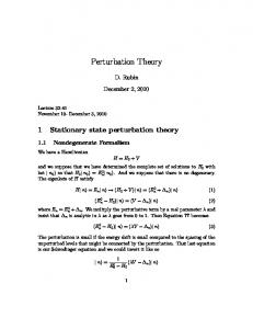
where P (z) is extracted directly from the images. The function φ(z) for an 1600 nm thick gold film is shown in fig. 1. The inset shows the probability density function f (z) = dP/dz = (1−P )dφ/dz. Similar behavior is realized for all investigated gold films. It is clear that for large positive z the logarithm of the phase can be fitted with a linear function ln φ(z) = A + Bz,

z→∞

(3)

and similarly for large negative z. With this φ the probability to find a feature larger than z behaves asymptotically as a double exponential    z−µ , (4) 1 − P (z) ∼ exp − exp β where β and µ are the scale and location parameters respectively. This behavior is a characteristic feature of the Gumbel distribution [23], which is an example of extreme value statistics. In this paper only gold films were analyzed and therefore we cannot draw conclusions on the roughness statistics of other materials. However, the extreme character of the statistics allows us to hope that this behavior is more general.

Roughness correction to the Casimir force. – We can imagine a rough surface as a large number of asperities with heights ∼ w and lateral size ξ, and occasional Statistics of rough surfaces. – The distance upon high peaks and deep troughs. These peaks (or troughs) are contact d0 was discussed in detail for gold films [21]. The high in the sense that their height is considerably larger films deposited with different thicknesses have different than w, say > 3w. The situation can be visualized as a rms roughnesses due to kinetic roughening processes. For lawn covered with grass and occasional high trees standing all these films atomic force microscope (AFM) images were here and there. In this paper we propose a method to calrecorded for large area (of up to 40 × 40 µm2 ) with lateral culate the roughness correction to the Casimir force on the resolution of 4-10 nm. This information allows a detailed basis of this separation. Namely, the asperities with the analysis of the roughness statistics. The probability to height ∼ w can be taken into account using perturbation find a height of a local feature smaller than some value z theory, without the use of the proximity force approximacan be presented in a general form tion. On the other hand, for high peaks the local distance P (z) = 1 − e−φ(z) , (1) between interacting bodies becomes considerably smaller and one cannot use perturbation theory anymore. Because where for convenience we introduced the ”phase” φ(z) as high peaks are rare the average distance l between them is nonnegative and nondecreasing function of z. The phase large. If this distance is so large that l ≫ d, then we can p-2

Roughness correction to the Casimir force beyond perturbation theory rough one, which has the combined roughness topography h(x, y) = h1 (x, y) + h2 (x, y), where h1,2 (x, y) are the topographies of the interacting plates 1 or 2. Therefore all the equations above have to be applied to the combined roughness profile h(x, y). Let us assume for a moment that the PFA can be applied to any roughness topography. Then the force between the plates can be calculated using the standard definition of the averaged function

2 w=10. 1 nm ξ=42 nm

−2

−2

log10f(z)

log10φ(z)

0

−4

−4 z (nm) −6 −40

−6 −40

0

40

F (d) =

80

Zd0

... +

d1

′ −d Z 1

... +

−d′0

Zd1

dzf (z)F (d − z),

(8)

−d′1

where f (z) is the probability density function, and we separated high peaks (first integral), deep troughs (second inFig. 1: (Color online) The “phase” as a function of z for a 1600 tegral), and the normal roughness contribution (third intenm gold film. The open circles are the actual data extracted gral). For the moment we do not specify the force between from the AFM image using eq. (2). At large positive and large the interacting patches F (d) separated by the distance d. negative heights log10 φ(z) is well fitted by linear functions of The last term can be calculated using the perturbation z as is shown by the straight lines. The curved line is a poly- expansion F (d − z) = F (d) − F ′ (d)z + F ′′ (d)z 2 /2! + . . . nomial fit at intermediate z. The inset shows the probability and we find for this term −20

0

20 40 z (nm)

60

80

density function f (z). It demonstrates significant deviation from a normal distribution.

calculate the contribution of these peaks independently of each other, as it is assumed in the PFA. However, this contribution has to be calculated beyond the perturbation theory. It has to be stressed that the interaction of a separate peak with a flat surface can be taken into account precisely using developed numerical or analytical methods [3]. The number of asperities N with the height d1 > 3w and lateral size ξ on the area L2 is given by the equation [21] L2 N = 2 e−φ(d1 ) . (5) ξ The average distance between these peaks is L l = √ = ξeφ(d1 )/2 . N

(6)

In order to fulfill the condition of PFA applicability l ≫ d, we can choose the parameter d1 from the interval 3w < d1 < d0 , where d0 is the maximal peak on the area L2 . The best choice for d1 will be discussed later. Similarly, one can introduce the average distance l′ between deep troughs L ξ l′ = √ = p , (7) N′ φ(−d′1 )

where d′1 has to be chosen from the interval 3w < d′1 < d′0 to fulfill the condition l′ ≫ d and d′0 is the deepest trough on the area L2 . Here we consider the general case where we are interested in the Casimir force between two plates with rough surfaces. As was explained in ref. [21] this is equivalent to the interaction of a smooth plate with a

Zd1 −d′1

. . . = F (d)

Zd1

−d′1

F ′′ (d) dzf (z) + 2!

Zd1

dzf (z)z 2 .

(9)

−d′1

The first and second integral on the right are 1 and w2 , respectively, if one extends the integration limits to infinity. When the applicability of the PFA breaks down the second term in (9) (with infinite limits) can be generalized as follows [17] Z F ′′ (d) d2 k FP T (d) = ρ(kd)σ(k). (10) 2! (2π)2 Here σ(k) is the Fourier spectrum of the roughness correlation function. The function ρ(kd) measures the deviation from the PFA. When the PFA is applicable this function is ρ(kd) = 1 and we reproduce eq. (9). Outside of the PFA applicability we can use for ρ(kd) expressions found in [18, 19]. The term FP T (d) is the roughness contribution to the force treated as a perturbation theory correction. As we know already the contribution of high peaks (or deep troughs) may not be accounted for by the perturbation theory. However, in this case we can account for the peaks (troughs) independently and the contribution can be presented as the first (second) term in (8). Taking into account the change of the integration limits we find the contributions due to high peaks, FP F A (d), and due to deep troughs, FP′ F A (d),

p-3

FP F A (d) = h Rd0 dzf (z) F (d − z) − F (d) + F ′ (d)z − d1

F ′′ (d) 2 2! z

i

, (11)

Wijnand Broer et al. FP′ F A (d) =

to keep in mind that FP F A decreases very fast with d and the absolute error stays small. The parameters d1 and d′1 i h R F ′′ (d) 2 ′ dzf (z) F (d − z) − F (d) + F (d)z − 2! z .(12) can be chosen rather arbitrarily if the conditions l(d1 ) ≫ d −d′0 and l(d′1 ) ≫ d are fulfilled. A practical recipe could be d1 = max [3w, (d0 + w)/2] and d′1 = max [3w, (d′0 + w)/2]. The final expression for the force that includes the total It has to be noted that the contribution of deep troughs roughness contribution can be presented as is always small, but we keep it for the sake of generality. −d′1

F (d) = F (d) + FP T (d) + FP F A (d) + FP′ F A (d).

(13)

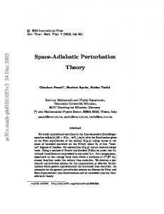
Results. – The roughness corrections (10)-(12) were deduced for the force between two rough parallel plates. In Here F (d) is the force between flat surfaces and the other most of the experimental configurations the sphere-plate three terms are the different roughness corrections. geometry is used. We can find the result for this configuraThe same force F (d) is used to calculate FP F A (d) and tion if the sphere’s radius is large, R ≫ d. This condition FP′ F A (d), which implies that high peaks are described as is typically true when the roughness effect is appreciable pillars with flat faces. However, this approximation is and we can apply the PFA to the total force F (d). The not necessary. If the peaks can be considered as inde- same equations (10)-(13) can be applied but now we have pendent, then the interaction of each peak with the flat to understand F (d) as the force between a smooth sphere surface can be described precisely (numerically) or approx- and a smooth plate, approximated by imately with an appropriate force F˜ (d) in eqs. (11) and (12), taking into account the actual geometry of the peak. F (d) = 2πRE(d) R ≫ d, (16) For example, high peaks can be considered as pillars with spherical caps of radius ξ/2. As we will see below for the where E(d) is the Casimir-Lifshitz energy per unit area description of the experiment [20] it is sufficient to use the for the parallel plate configuration [9]. We neglect the thermal effect (T = 0) at short separations [12]. However, simplest model for the peaks (flat faces). At this point an important question is: with what pre- we use measured optical properties of gold films [11] to cision can we calculate the roughness corrections? The account for the actual material properties. We evaluated the force and all the roughness correcterm −F ′′′ (d)z 3 /3!, which is neglected in the Taylor expansion of F (d − z), allows an estimation of the error in tions to compare it with the experimental data [20]. The FP T . In the distance range that we are interested in here, Lifshitz force F (d) was calculated for the sphere radius 20 < d < 100 nm, the force F (d) behaves with the dis- R = 50 µm using the optical data for sample 3 in [11]. tance as F (d) = A/dα , where A is a constant and α ≈ 3.5 The roughness effect was estimated for 800, 1200, and 1600 nm Au films and a Au covered sphere. Here we present [24]. Then the error is estimated as the results for the 1600 nm film. The roughness charα(α + 1)(α + 2)  w 3 ∆FP T = γ F (d), (14) acteristics for combined sphere-plate AFM images were 3! d presented in ref. [21]. For the 1600 nm film they are: rms roughness w = 10.1 nm, the correlation length ξ = 42 nm, where γ is the skewness of the distribution f (z). The and the distance upon contact d0 = 50.8 ± 1.3 nm. The data shown in fig. 1 give the largest γ = 1.285 among the last value was determined by electrostatic calibration [20]. investigated films and we estimate the error as ∆FP T ≈ It is preferable to use this value, because d0 determined 3 18.55(w/d) F (d). The latter means that the perturbation from the roughness topography has a larger uncertainty theory correction has meaning at least for d/4 > w. The [21]. We used d1 = (w + d0 )/2 = 30.5 nm. According minimal distance between rough surfaces d0 depends on to eq. (6) it corresponds to the average distance between 2 the area of nominal contact L , but even for L as small high peaks, l ≈ 380 nm. Note that the effective area of in2 as 1 µm the condition d0 /w > 4 is usually fulfilled [21]. teraction is L2 , with L = 2100 nm [21]. For deep troughs Therefore, we can now draw the important conclusion that the calculation details are less important. For the given the perturbation theory correction (10) has meaning up to L we found d′0 = 24.6 nm. Since d′0 < 3w the troughs are the point of contact between interacting rough surfaces. not deep enough and can be taken into account perturbaThe precision with which we calculate the contribution tively. Therefore, in this specific case there is no need to of the high peaks is defined by the condition of applicabilintroduce FP′ F A . ity of the PFA to these peaks. This condition is l(d1 ) ≫ d The results are presented in fig. 2. One can see that the and we have for the error solid (blue) line, which shows the result of our approach, is ∆FP F A = (d/l) FP F A . (15) in agreement with the experimental data within the experimental errors. This is in contrast with the perturbation As we already mentioned we have to choose d1 such that theory approach that failed to explain the data [20]. This the condition l(d1 ) ≫ d is true and, therefore, the correc- is demonstrated in the inset, which shows different comtion (11) makes sense. Similarly, we can define the error ponents of this force. At short distances the contribution ∆FP′ F A for the contribution of deep troughs (12). The rel- of high peaks (2, red) is so large that it dominates the ative error in (11) increases with the distance, but we have whole force. In this case a few peaks become very close p-4

Roughness correction to the Casimir force beyond perturbation theory be [17]. However, the difference between these two curves is within the experimental errors. Perturbation theory accounts for the non-additivity of the Casimir force, whereas the PFA assumes it is additive. So this difference provides an indication of the effect of the non-additivity in the roughness correction. It can be concluded that within the experimental error the experiment in ref. [20] was not sensitive to this non-additivity.

1 0.4

0.6

0.3 Force (nN)

Force (nN)

0.8

0.2

1 2

0.1 0

0.4

50

3 60

70

80

90

100

d (nm)

0.2

0

50

60

70

80 d (nm)

90

100

Fig. 2: (Color online) The force between a Au covered sphere (R = 50 µm) and a plate (1600 nm thick Au). The open (green) circles are the experimental data from [20]. The vertical and horizontal bars show the experimental errors for a few points. The solid (blue) line is the result of our model. Naive application of the PFA to the force between rough bodies based on eqs. (8) and (16) is shown by the dashed (red) curve. The inset shows different components of the force. 1 (black) is the force F (d) between smooth surfaces calculated according to the Lifshitz formula. 2 (red) is the contribution of the high peaks according to eq. (11). 3 (blue) is the perturbation theory correction according to eq. (10). The sum of all three curves gives the solid line in the main panel.

to the opposite body so that the force diverges at d → d0 . There can be very few high peaks but their contribution cannot be neglected. On the other hand the contribution of high peaks disappears very fast when the distance becomes larger. We used two different models to calculate the contribution of high peaks in eq.(11). In the first model the peak was considered as a pillar with a flat face. In the second model the peak had a spherical cap of radius ξ/2. The interaction of the cap with a plate was taken into account according to ref. [25], where the proximity force approximation is not used. We found a negligible difference between the two models of peaks. The reason is the following: When the distance d − d0 ∼ ξ, then the contribution of the peaks is very small due to their small area of interaction. When d approaches d0 or d− d0 ≪ ξ, the contribution of high peaks becomes significant, but the shape of the peaks is not important anymore, because the PFA is valid in this limit. Naive application of the proximity force approximation according to eqs. (8) and (16) gives the dashed line (red) in fig. 2. It is interesting to note that this line is also in agreement with the experimental data. At the shortest separations both curves coincide, because the dominating high peaks can be treated with the PFA. At larger distances the perturbative contribution becomes important and the PFA result lies below the solid line as it should

Conclusions. – In conclusion, we developed a reliable method to include the effect of roughness of interacting bodies in the Casimir force at short distances when perturbation theory fails. It was established that roughness of gold films can be described asymptotically (for high peaks or deep troughs) by extreme value statistics. In this case the rough surface can be presented as a large number of asperities with heights of the order of the rms roughness and a few occasional peaks, which are much higher than the rms roughness. The distance between high peaks is large so that one can calculate their contribution for each peak separately (using the PFA). The smaller asperities can be calculated using perturbation theory beyond the PFA. The contribution of high peaks is extremely important for short separations, where it dominates not only the perturbative roughness correction but also the force as a whole. Therefore, our result is interesting not only for the Casimir force but also for the problem of adhesion between surfaces in general [26], including wet environments [27–29]. We repeat that the method presented here solves the significant discrepancy between measurements of the Casimir force at short separations, and the results of perturbation theory [20]. ∗∗∗ The authors benefited from exchange of ideas within the ESF Research Network CASIMIR. We would also like to thank P. J. van Zwol and B. J. Hoenders for useful discussions. REFERENCES

p-5

[1] H. B. G. Casimir, Proc. K. Ned. Akad. Wet. 51, 793 (1948). [2] F. Capasso, J. N. Munday, D. Iannuzzi, and H. B. Chan, IEEE J. Sel. Top. Quantum Electron. 13, 400 (2007). [3] A. W. Rodriguez, F. Capasso, and S. G. Johnson, Nature Photon. 5, 11 (2011). [4] P. Ball, Nature 447, 772 (2007). [5] F. M. Serry, D. Walliser, and G. J. Maclay, J. Appl. Phys. 84, 2501 (1998). [6] E. Buks and M. L. Roukes, Europhys. Lett. 54, 220 (2001). [7] E. Buks and M. L. Roukes, Phys. Rev. B 63, 033402 (2001). [8] I. E. Dzyaloshinskii, E. M. Lifshitz and L. P. Pitaevskii, Advances in Physics 38, 165 (1961).

Wijnand Broer et al. [9] E. M. Lifshitz and L. P. Pitaevskii, Statistical Physics (Pergamon Press, Oxford, 1980) Pt. 2. [10] A. Lambrecht and S. Reynaud, Eur. Phys. J. D 8, 309 (2000). [11] V. B. Svetovoy, P. J. van Zwol, G. Palasantzas, and J. T. M. De Hosson, Phys. Rev. B 77, 035439 (2008). [12] K. A. Milton, J. Phys. A: Math. Gen. 37, R209 (2004). [13] A. O. Sushkov, W. J. Kim, D. A. R. Dalvit, and S. K. Lamoreaux, Nature Phys. 7, 230 (2011). [14] G. L. Klimchitskaya and Yu. V. Pavlov, Int. J. Mod. Phys. A 11, 3723 (1996). [15] B. V. Derjaguin, Kolloid Z. 69, 155 (1934). [16] B. V. Derjaguin, I. I. Abrikosova, and E. M. Lifshitz, Quart. Rev. Chem. Soc. 10, 295 (1956). [17] C. Genet, A. Lambrecht, P. Maia Neto and S. Reynaud, Europhys. Lett. 62, 484 (2003). [18] P. A. Maia Neto, A. Lambrecht, and S. Reynaud, Europhys. Lett. 69, 924 (2005). [19] P. A. Maia Neto, A. Lambrecht, and S. Reynaud, Phys. Rev. A 72, 012115 (2005). [20] P. J. van Zwol, G. Palasantzas, and J. Th. M. De Hosson, Phys. Rev. B 77, 075412 (2008). [21] P. J. van Zwol, V. B. Svetovoy, and G. Palasantzas, Phys. Rev. B 80, 235401 (2009). [22] S. Coles, An Introduction to Statistical Modelling of Extreme Values (Springer, Berlin, 2001). [23] E. J. Gumbel, Statistics of Extremes (Dover Publications Inc., 2004). [24] G. Palasantzas, V. B. Svetovoy, and P. J. van Zwol, Int. J. Mod. Phys. B 24, 6013 (2010). [25] A. Canaguier-Durand, P. A. M. Neto, I. Cavero-Pelaez, A. Lambrecht, and S. Reynaud, Phys. Rev. Lett. 102, 230404 (2009). [26] F. W. DelRio, M. P. de Boer, J. A. Knapp, E. D. Reedy, Jr., P. J. Clews, and M. L. Dunn, Nature Mater. 4, 629 (2005). [27] F. W. DelRio, M. L. Dunn, L. M. Phinney, and C. J. Bourdon, Appl. Phys. Lett. 90, 163104 (2007). [28] P. J. van Zwol, G. Palasantzas, and J. T. M. De Hosson, Phys. Rev. E 78, 031606 (2008). [29] B. N. J. Persson, J. Phys.: Condens. Matter 20, 315007 (2008).

p-6