Routing in Multi-Sink Sensor Networks Based on Gravitational Field

The 2008 International Conference on Embedded Software and Systems (ICESS2008)

Routing in Multi-Sink Sensor Networks Based on Gravitational Field※ Jinbao Li, Shouling Ji, Hu Jin and Qianqian Ren School of Computer Science and Technology Heilongjiang University, Harbin, China {jbli, slji, hujin}@hlju.edu.cn

the sink through other mid-sensors. Sinks could communicate with the satellite, and by this way, users can interact with the networks. In the present, some researchers map the problems in sensor networks to the classical physical problems, and solving these problems by the mathematicsphysics methods. S.Toumpis and other researchers studied the optimal design and operation of massively dense wireless networks. They abstract the problem to the distributing problem of electric charges in the electrostatics. The networks optimal deployment conditions can be obtained through the charges distributing characteristic in the electrostatic field[1]. In [2,3], they studied this problem farther more, which equipped with a general physical layer. M.Kalantari and M.Shayman studied the routing problem in Ad Hoc networks by analogy to electrostatic theory. In this abstracted electrostatic field, the authors get a series of Partial Differential Equations (PDEs) based on the properties of electrostatic field. By solving these PDEs, they can get the corresponding route of every sensor[4]. The same authors continued their work in [5]. In this paper, they studied the optimal design problem of Multi-Sink Sensor Networks also by analogy to electrostatic theory. In [6], they expanded their work to MultiCommodity sensor networks; they proposed a routing method based on PDEs in this paper. But, the algorithms based on PDEs have many disadvantages. Generally, we can get the PDEs’ numerical results only in some special conditions, and the cost to figure out the PDE is too high. So, in the actual sensor networks, it is almost impossible to solve Partial Differential Equations by the present nodes. A method to deploy multiple sinks in the sensor networks based on an electrostatic model was proposed in [7]. This method can accommodate the electric charges’ type and amount of the sensors dynamically,

Abstract The process of data forwarding in sensor networks is analogy to electric charge moving in electrostatic field. By this analogy, a method which abstracting a sensor networks to a Gravitational Field is proposed in this paper. In this gravitational field, sink node has gravitational to the data and data can flow to sink under this gravitational. Based on this gravitational field, a routing method which applies well in MultiSink sensor networks is proposed in this paper. This method has a lower time and space complexity, and it can adapt to the variety of the networks size dynamically. Theoretic analysis and simulation results indicate that: the routing method this paper proposed can decrease the energy consuming of data transmission effectively, reduce the data packet discard rate, uniform the networks’ loads, and prolong the lifecycle of the networks.

1. Introduction As the development of communications technology, embedding technology and microelectronics technology, sensor networks have been studied extensively in recent years. This networks have many applications including military, environment monitoring, medical treatment, building status monitoring and intelligence furniture and other many fields. A typical sensor networks is composed of sensor nodes and sink nodes. Generally, sensors’ computing capability, communicating ability and storage memory are weaker, sinks have more resources, they have enough processing power, storage space and capability of communicating. When a sensor node senses an event, it should forwarding the data to ※

This paper has been supported by the Natural Science Foundation of Heilongjiang Province of China under Grant No.QC04C40.

978-0-7695-3287-5/08 $25.00 © 2008 IEEE DOI 10.1109/ICESS.2008.14

368

by this way, it can build an energy-efficient networks. This method considers the residual energy mostly; when the mobile sinks change its place. But it ignores the environments of the networks running. In [8], a decentralized service discovery mechanism for ad hoc networks, which uses the field theoretic approach, was proposed. This method uses the positive and negative charge to model the service and service request separately; the service request can find its route to the destination through the potential values of its neighbors. In [9], a simple Magnetic Diffusion (MD) mechanism based on magnetic filed was proposed. In this method, the sink is modeled by magnet and the data is modeled by metallic nails, and data can be forwarded to the sink according to the magnetic charge of every node. MD method can perform well in timely delivery data, achieve high data reliability and energy efficiently, but MD could not use the networks resources uniformly. A routing method by analogy to Geometrical Optics was proposed in [10, 11]. This method abstracts the process of data transmission in networks as the light spreading in some media with different refractive index. After considering the energy consuming, load balancing and the lifecycle and other problems in the networks synthetically, we proposed a routing method in Multi-Sink sensor networks based on field theory in this paper. This method abstracts the sensor networks to a gravitational field generated by sinks, and it uses gravitational field intensity to denote the communication attributes of every sensor. And this method can choose the next-hop for all the sensors based on the gravitational field intensity of its neighbors. Theoretic analysis and simulation results indicate that compared with other similar algorithms, the routing method this paper proposed has a lower computational complexity, a lesser energy consuming and can improve the routing efficiency significantly. And the experiment results proved that it can adapt the Multi-Sink sensor networks well. The remainder of this paper is organized as follows: in Section 2 we proposed the routing method in MultiSink sensor networks based on gravitational field, and we analyze its performance in this section too. In Section 3, we give some experiments, and compare the results with some other methods. And we conclude the paper in Section 4.

2. Routing mechanism gravitational field

based

upper limit of networks load is known in some region; (2) the initial energy of a node is known, and the residual energy is known at any moment; (3) sink can communicate with the satellite, users can access the data via satellite. Before the formal discussions, we make the following definitions first. Definition 1: Monitoring Area of Sensor. The monitoring area of a sensor is a round region, and its radius is smaller than the sensor’s communications radius. Definition 2: Load of Sensor. The total amount of data generated in the monitoring area of a sensor is the load of sensor. Definition 3: Monitoring Area of Sink. If a sensor’s data is transmitted to the sink, then the monitoring area of this sensor is belonged to the monitoring area of this sink. The monitoring area of a sink is equal to the total monitoring area of all sensors, which transmit their data to this sink. Definition 4: Load of Sink. The total amount of data generated in the monitoring area of a sink is the load of sink.

2.1. Definition of gravitational field We know from electromagnetism, electric charge can generate electrostatic filed, and it has strength effect to other charges in this filed. Suppose that an electrostatic field is generated by a negative charge, and then it has an attraction to a positive charge in this filed. The positive charge moves toward to the negative charge under this attraction. Consider the data flows form the sensor to the sink by multi-hop way in the sensor networks; it is analogy to the charges interaction and moving in the electrostatic field. By this analogy, we make the following abstracting: The data that monitored by sensors is modeled by positive charge with appropriate magnitude; the sinks are modeled by negative charge with appropriate magnitude, and sinks have attraction to the data. In this way, the networks is abstracted to a field generated by sinks. In this field, sensors may generate data randomly, and sinks have attraction to these data, and the data can flow to the sinks under this attraction. By the analogy to charges moving in electrostatic field, we give the definition of Gravitational Field, Attraction of Data, and Gravitational Field Intensity first time in the following. Definition 5: Gravitational Field (GF). Consider a single-sink sensor networks deployed in area A, the coordinate of the sink is (xs,ys). Then, if a sensor in the networks monitors some data, the data transmission can abstract as: sink has an attraction to the data, and

on

According to the actual applications of sensor networks, we make the following assumptions: (1) the

369

the data will flow to the sink under this attraction. In this way, the networks deployed in area A is abstracted as a Gravitational Field generated by the sink in (xs,ys). Definition 6: Attraction of Sink (AoS). After the above abstracting process, for a sensor in the networks which coordinate is (x,y), define the Attraction of Sink to the data sensed by this sensor as follow: G Q ⋅ q ( x, y ) (1) F ( x, y ) = k ( x, y ) rˆ

and these M sinks generate a Gravitational Field in Area A together. For a sensor in this network which coordinate is (x,y), the Attraction of Sink to the data in this sensor is: M G G G G G F ( x, y) = F1 ( x, y ) + F2 ( x, y ) +" + FM ( x, y) = ∑ Fi ( x, y) (5) i=1

G in which Fi ( x, y) is the attraction generated by the ith sink. Then, the GFI of the sensor in (x,y) is: M G G G G Q C(x, y) = C1(x, y) + C2 (x, y) +"+CM (x, y) = ∑k(x, y) 2i rˆi (6) ri i=1 in which Qi is the load of the ith sink; ri is the logistic distance between (x,y) and the ith sink.

r2

in which rˆ is an unit vector, and it denotes the direction of the attraction; Q is the load of sink; q(x,y) is the unit load, namely, the data amount generated in per unit of area per unit of time. r is the logistic distance between the sensor in (x,y) and the sink. The definition of r is: (2) r = dis ( xs , ys , x, y ) ⋅ w( x, y ) in which dis(xs,ys,x,y) is the physical distance between (x,y) and sink. w(x,y) is the environment function in location (x,y), which reflects the influences to the communications brought by landform, physiognomy, barrier, the weather conditions and other environment factors. Consider the environmental characteristics, can illuminate the communications capacity of a certain place better. k(x,y) in Equation(1) is the energy function, its definition as follow: E ( x, y ) (3) k ( x, y ) = a f

2.2. Routing mechanism based on gravitational field 2.2.1. Solving of GFI. Form the definition of GFI in section 2.1 we know: when compute the GFI of every sensor, we don’t consider its neighbors, but only consider the residual energy, the environmental characteristics, Etc. of the current node. So, we can figure out the GFI of every sensor in the networks by a distributed parallel algorithm. Consider a Multi-Sink sensor networks contains m sinks and n sensors. In order to get the GFI of the n sensors, we only need these n sensors calculate equation (6) respectively. We propose the following Gravitational Field Intensity Algorithm (GFIA) to calculate the GFI of every node. The basic thinking of GFIA is: i) for every sensor, compute the components of GFI separately generated by every sink; ii) compute the vector adding result of these GFI components, and the eventually result is the sensor’s GFI. In the following GFIA, GraInten is the data structure of GFI, and it composed by the magnitude of GFI, the direction of GFI, Etc. NodeInfo is the data structure of node information. It contains the node’s coordinate, residual energy and the information of surroundings. Algorithm 1: Gravitational Field Intensity Algorithm (GFIA) GravitationalIntensity( i ) 1:GraInten G_i = Null, g; 2:NodeInfo sensor_i, sink[m]; 3:for sensor i 3.1: for (j=0; j0, Adjacency Azimuth Angle B=0; 4: compute the Azimuth Region A-area corresponding to S(x,y); 5: while (A+B≤ 2π ) 5.1: compute the Adjacency Azimuth Region Barea corresponding to S(x,y); 5.2: initialize Sneighbor according to A-area and Barea; 5.3: set Snext_hop=NULL, the GFI of Snext_hop |GD|=|the GFI of S(x,y)|; 5.4: while ( Sneighbor != NULL ) 5.4.1: take a node S(x*,y*) form Sneighbor; 5.4.2: if(S(x*,y*) is a sink ) 5.4.2.1: Snext_hop= S(x*,y*),break; 5.4.3: else if (the GFI of S(x*, y*) |GD*|> |GD| ) 5.4.3.1: |GD|=|GD*|, Snext_hop= S(x*, y*); 5.4.4: Sneighbor=Sneighbor-{S(x*,y*)}; 5.5:if (Snext_hop != NULL ) 5.5.1: return Snext_hop; 5.6: else 5.6.1:A+=B,reset Adjacency Azimuth Angle B>0; At the beginning of the above algorithm, OBNH sets the Adjacency Azimuth Angle to be 0, and searches the next-hop in the Azimuth Region A-area. Take the sensor which coordinate is (x,y) in Fig.1 as an example, OBNH search the next-hop in the neighbor nodes set {S1,S2} first. If OBNH can find the appropriate next-hop in this set, it will end after returning the appropriate next-hop. Else, OBNH will search the next-hop in the Adjacency Azimuth Region B-area. In Fig.1 the neighbor nodes set corresponding to B-area is {S3,S4,S5,S6}. If the OBNH still can’t find the appropriate next-hop, it will reset the Adjacency Azimuth Angle and the Adjacency Azimuth Region again until find the appropriate next-hop.

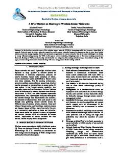
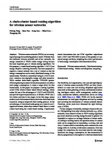
3. Simulation results and analysis Suppose there is a sensor networks deployed in an area. Sensors uniformly distributed and sinks randomly distributed in the networks. For the simplicity of the experiments, here we consider a networks deployed in a 19×19 grid. There are 4 sinks and 257 sensors in the networks, and the coordinates corresponding to each sink are: (x1,y1)=(9,9), (x2,y2)=(15,15), (x3,y3)=(13,5), (x4,y4)=(5,15). Suppose the upper limit of networks load is 100, and the load distributes uniformly in the networks, and the initial load of every sink is the same. Suppose the surroundings of nodes in the networks are same, i.e. w(x,y) is a constant. Furthermore, we set energy function k(x,y)=1 in our experiments. We obtained the GFI of every sensor in the networks as shown in Fig.3 by using GFIA proposed in section 2.2.1. The direction of GFI in every sensor is shown in Fig.4. By running OBNH, we can get the route corresponding to each sensor. And the weights of each sink are: Q(x1,y1)=29.6399, Q(x2,y2)=21.8836, Q(x3,y3)=25.2078, Q(x4,y4)=23.2687. In order to study the method proposed in this paper further, we study the performance of this method when it works in different sensor networks with different sinks. And we will compare its performance with Directed Diffusion (DD) [12] Algorithm and the Flooding Algorithm. Suppose there are 19×19 nodes in the networks, and the deployment of the networks is similar to the settings of the above experiment but with different sinks in numbers and locations. The surroundings of nodes in the networks are same. The initial energy of a sensor is 1000 units, and the initial energy of a sink is 100000 units. Sensors are uniformly distributed in the networks and sinks are randomly distributed in the networks.

2.3. Performance analysis To the GFIA proposed in this paper, by the analysis in section 2.2.1, the complexity of computing time and space are all between the constant level and polynomial level, and it only rely on the number of sinks in the networks. Therefore, the routing method

20 15 10 5 0 2

4

6

8 10 12 14 X

20 18 16 14 12 10 8 6 4 2 Y

gra vitation intensity

25

16

18

20

Figure 3. GFI of every sensor in the networks

372

time, and DDw denotes the networks will not update its routing in the whole life cycle. In Fig.5, Flooding denotes the networks works in Flooding algorithm, and this is almost to say the networks almost has no routing mechanism. When the networks adopts DD algorithm, each routing updating process will consume a lot of energy. Hence, let the networks choose different routing updating cycle or without routing updating is in the pursuit of the largest energy-efficiency. Of course, this is at the expense of the increasing of Packet Discarding Rate; it is impossible in the actual sensor networks. Here, we just want to compare the biggest task may be completed by the networks working different protocols. From Fig.5 we know: when the networks has less sinks, GFIA has no superiority relative to DD, but when the networks has more sinks, GFIA can accomplish more monitoring task than DD obviously. This is because GFIA consider the load of every sink synthetically, and it chooses the optimal net-hop with the biggest GFI in its neighbor nodes, hence it can choose an more balanced efficient route. The Flooding’s performance is very poor compared to GFIA and DD, this is because it will transmit each packet it sensed to the surroundings in a flooding way, it will cost so much energy that the energy of these nodes around sinks will depleted rapidly, and the life cycle of the networks will end. In the following discussing, if it has no explanations specially, the meaning of GFIA, DD1, DD2, DDw and Flooding is same as in Fig.5. Fig.6 shows the average monitoring packets of per sink when the i-sink networks work in different routing mechanisms. In which, x-axis denotes different networks with different number of sinks; y-axis denotes the average number of packets sensed by per sink. Form Fig.6 we know: if DD has a long routing updating cycle, the average number of packets sensed by per sink is more. If the networks has less sinks, DD is better than GFIA. But when the networks has more sinks, because GFIA can use the networks resources more uniformly, it is better than DD. And the average number of packets monitored by every sink can be maintained at around 4400. Certainly, when the number of sinks achieves a certain magnitude, it will lose its meaning to add sinks more. Fig.7 shows the average hops of the packets form being generated to be transmitted to a sink. In which, x-axis denotes different networks with different number of sinks; y-axis denotes the average hops of the packets. We can see from Fig.7, the average hops of data packets decrease as the increase of sinks. The average packets hops of GFIA is more than DD, the reason can be obtained form Fig.7. When GFIA chooses routes for some sensors, it chooses a longer path. This choice can not only avoid congestions and

20 18 16 14 12

Y

10 8 6 4 2 0 0

2

4

6

8

X

10

12

14

16

18

20

Figure 4. Directions of the GFI in every sensor The networks will generate an event per unit time, and the data amount to describe an event is 1 data packet. The event will generate randomly, and it can be sensed by the nearest node. If an event has two or more nearest nodes, then it can be sensed by one of these nearest nodes in the same probability. Of course, if the event’s nearest nodes contain a sink; it will be sensed by the sink preferentially. Monitoring an event successfully will cost 1 unit energy, and transmitting or receiving a data packet will cost 1 unit energy separately too. Suppose a sensor can only communication with its directly adjacent neighbors, its biggest communication radius is 2 , i.e. the directly adjacent neighbors of a sensor can be 3, 5 or 8. In order to compare different networks with different number of sinks and working in different routing methods, here we consider the scenarios of networks has 1-sink to 10sink severally. In which, i-sink denotes a sensor networks with i sinks. Before the study, we make the following definitions first: Definition 12: Life Cycle of Sensor Networks. The Life Cycle of Sensor Networks begins with the deployment of the networks and will end if all the sinks in the networks can not receive any data packets. Definition 13: Packet Discarding Rate. If a data packet can’t be transmitted to the sink, and then it will be discarded. The ratio of data packets discarded and the total amounts of data packets is defined as Packet Discarding Rate. When the above i-sink(1 ≤ i ≤ 10) networks working in the routing method (we denote it by GFIA) proposed in this paper, DD algorithm and Flooding algorithm separately, the biggest total load of different networks shown in Fig.5. In Fig.5, x-axis denotes different networks with different number of sinks; yaxis denotes the total load that the networks can take on. GFIA denotes the networks works in the method this paper proposed. DD1, DD2 and DDw denote the networks work in DD algorithm, but with different routing updating cycle. DD1 denotes the networks will update its routing per 1000 units’ time; DD2 denotes the networks will update its routing per 2000 units’

373

reduce conflicts but also use the energy more uniformly. The average energy cost of every data packet is shown in Fig.8. In Fig.8, x-axis denotes different networks with different number of sinks; yaxis denotes the average energy cost of every packet. As the increase of sinks, the average hops of every packet is decrease, hence the average energy cost is depressed too. Although the average hops of packets in GFIA is more, its average energy cost is lower than DD. This is because the Packet Discarding Rate is higher; it wastes a lot of energy. And DD updates its routing periodically; it also consumes part of the additional energy. We give the Packet Discarding Rate of 4-sink networks in Fig.9.

average hops of packet

6

30000

3 2

10000

1

2

3

1

2

4

5

6

7

8

number of sinks in networks

9

10

0.7

4100 4000 3900 3800 3700 3600 3500 4

7

8

9

10

5

6

7

8

n um ber of sinks in netw orks

9

2

3

4

5

6

7

8

number of sinks in networks

9

10

GFIA DD1 DD2 DDw

0.6

4200

discard rate of packets

average loads of sink(packets)

4400 4300

3

6

Figure 8. Average energy cost of every data packet

GI DD1 DD2 DDw

4600 4500

2

5

GFIA DD1 DD2 DDw

1

1

4

85 80 75 70 65 60 55 50 45 40 35 30 25 20 15 10 5

Figure 5. Total monitoring tasks of i-sink networks

3400

3

number of sinks in netw orks

Figure 7. Average hops of data packets

20000

0

4

1

GFIA DD1 DD2 DDw Flooding

40000

GFIA DD 1 DD 2 DD w

5

energy

load of networks(packets)

50000

lower Packet Discarding Rate, and its load balancing effect is more better and it can prolong the lifecycle of the networks by increasing the total tasks that can by accomplished by the networks.

10

0.5 0.4 0.3 0.2 0.1 0.0

Figure 6. Average monitoring packets of per sink

0

20000

40000

60000

80000

number of sensed packets

100000

Figure 9. Packet discarding rate of 4-sink networks

In Fig.9, x-axis denotes the packets number monitored by the 4-sink networks; y-axis denotes the Packet Discarding Rate. From this Fig. we can see: the Packet Discarding Rate of GFIA is far less than DD. This is because in order to use energy more uniformly, GFIA will choose longer paths for some sensors. Certainly, these choices will decrease the congestions and conflicts in the shorter paths. Hence, GFIA has a lower Packet Discarding Rate. According to the comparisons of different performance parameters in different i-sink sensor networks above, we can obtain that: in a Multi-Sink sensor networks, GFIA can consider various factors in the networks synthetically, hence it can use the energy of the networks more uniformly. Compared with DD and Flooding, the average energy cost of data transmission of GFIA is much less, and GFIA has a

4. Conclusions and future work We proposed a routing method (GFIA) in MultiSink sensor networks based on field theory in this paper. This method abstracts the sensor networks to a Gravitational Field generated by sinks. In this abstract field, sink had attraction to the data, and data can flow to the sink under this attraction. When study the problem above, this method considered the influences of the distance between sensor and sink, the residual energy of sensor, the environmental characteristics and other factors. Compared with the routing method based on PDEs, DD and Flooding: i) the computational complexity of GFIA is lower; ii) GFIA can adapt the changes of the networks size dynamically; iii) GFIA can solve the problems of energy-efficiency and load

374

balancing well. And GFIA can improve the performances of Multi-Sink sensor networks significantly. The future work includes solving some additional issues in GFIA. For example: the surroundings of sensors in the networks are impossible to be all the same. How to choose environment function need further study.

wireless networks”, in Proceedings of IEEE INFOCOM, Anchorage, AK, May 2007, pp. 1010-1018. [12]. C. Intanagonwiwat, R. Govindan and D. Estrin, “Directed Diffusion: A Scalable and Robust Communication Paradigm for Sensor Networks”, in Proceedings of 6th Annual Int’l Conf on Mobile Computing and Networks (MobiCOM 2000), Bostion, MA, Aug. 2000, pp. 56-57.

5. References [1]. S. Toumpis and L. Tassiulas, “Packetostatics: Deployment of Massively Dense Sensor Networks as an Electrostatic Problem”, in Proceedings of IEEE INFCOM, Miami, FL, Mar.2005, pp. 2290-2301. [2]. S. Toumpis and G. A. Gupta, “Optimal placement of nodes in large sensor networks under a general physical layer model”, in Proceedings of IEEE SECON, Santa Clara, CA, Sep.2005, pp. 275-283. [3]. S. Toumpis and L.Tassiulas, “Optimal Deployment of Large Wireless Sensor Networks”, IEEE Trans. Inform. Theory, Jul.2006, pp. 2935-2953. [4]. M. Kalantari and M. Shayman, “Routing in wireless ad hoc networks by analogy to electrostatic theory”, in Proceedings of IEEE International Communications Conference (ICC-04), Paris, France, June 2004, pp. 40284033. [5]. M. Kalantari and M. Shayman, “Design Optimization of Multi-Sink Sensor Networks by Analogy to Electrostatic Theory”, in Proceedings of IEEE WCNC. Las Vegas, NV, Apr. 2006, pp. 431-438. [6]. M. Kalantari and M. Shayman, “Routing in MultiCommodity Sensor Networks Based on Partial Differential Equations”, in Proceedings of Conference on Information Sciences and Systems, Princeton University, NJ, Mar.2006, pp. 402-406. [7]. Zoltán Vincze, Kristóf Fodor, Rolland Vida and Attila Vidács, “Electrostatic Modelling of Multiple Mobile Sinks in Wireless Sensor Networks”, in Proceedings of IFIP Networking Workshop on Performance Control in Wireless Sensor Networks, Coimbra, Portugal, May 2006, pp. 30-37. [8]. V. Lenders, M. May and B. Planttner, “Service Discovery in Mobile ad hoc Networks: A Field Theoretic Approach”, in Proceedings of the IEEE International Symposium on a World of Wireless Mobile and Multimedia Networks(WoWMoM), Taormina, Italy, June 2005, pp.120130. [9]. Hsing-Jung Huang, Ting-Hao Chang, Shu-Yu Hu and Polly Huang, “Magnetic Diffusion: Scalability, Reliability, and QoS of Data Dissemination Mechanisms for Wireless Sensor Networks”, in Computer Communications, Aug. 2006, pp. 2482-2493. [10]. R. Catanuto, G. Morabito and S. Toumpis, “Optical routing in massively dense networks: Practical issues and dynamic programming interpretation”, in Proceedings of International Symposium on Wireless Communications Systems, Valencia, Spain, Sep.2006, pp. 83-87. [11]. R. Catanuto, S. Toumpis and G. Morabito, “Opti{c,m}al: Optical/Optimal routing in massively dense

375