Row-wise Parallel Predicate Evaluation Ryan Johnson∗
Vijayshankar Raman
Richard Sidle
Garret Swart∗
C.M.U.
IBM Almaden Res. Ctr.
IBM Almaden Res. Ctr.
Oracle
[email protected]
[email protected]
[email protected] [email protected]
ABSTRACT
However, more and more data warehouses store tables denormalized, in main memory, often in compressed form. For such warehouses, joins and I/O are no longer the issue. Accessing the denormalized table is the main cost, and in many cases this cost is mainly that of predicate evaluation.
Table scans have become more interesting recently due to greater use of ad-hoc queries and greater availability of multicore, vector-enabled hardware. Table scan performance is limited by value representation, table layout, and processing techniques. In this paper we propose a new layout and processing technique for efficient one-pass predicate evaluation. Starting with a set of rows with a fixed number of bits per column, we append columns to form a set of banks and then pad each bank to a supported machine word length, typically 16, 32, or 64 bits. We then evaluate partial predicates on the columns of each bank, using a novel evaluation strategy that evaluates column level equality, range tests, IN-list predicates, and conjuncts of these predicates, simultaneously on multiple columns within a bank, and on multiple rows within a machine register. This approach outperforms pure column stores, which must evaluate the partial predicates one column at a time. We evaluate and compare the performance and representation overhead of this new approach and several proposed alternatives.
1.
1.1 Predicate Evaluation in Blink
INTRODUCTION
Complex predicates are a common feature of queries in data warehouses. The typical decision support query is generated by a tool, and involves an aggregation over a subset of the database, where the subset is defined by a conjunction of dozens of predicates, some of which may in turn involve complex expressions and nested disjunctions. E.g, the following is a WHERE clause from one of the simpler queries in a customer workload CUSTW1 that we use in this paper (the column names are anonymized and the query is varied slightly but the basic structure is unaltered): A = a AND B = b AND C IN (c,d) AND D = 0 AND E = 0 AND F = 2 AND H IN (e,f) AND (I IN (g,h) OR I > j) AND 9 other clauses (Q1) Traditionally, DBMSs have considered the principal bottlenecks in query speed to be I/O and joins, and so have not optimized much for predicate evaluation, other than applying them as early as possible in the query plan. ∗
Work done while author was at IBM
Permission to make digital or hard copies of portions of this work for personal or classroom use is granted without fee provided that copies Permission to copy without feefor all or part of material isadvantage granted provided are not made or distributed profit or this commercial and that copiesbear are not or distributed direct commercial thatthe copies thismade notice and the fullforcitation on the firstadvantage, page. the VLDB copyright notice and of the publication andthan its date appear, Copyright for components of the thistitle work owned by others VLDB and notice is must givenbe that copying is by permission of the Very Large Data Endowment honored. Base Endowment. To copy otherwise,Toorcopy to republish, to to post on servers Abstracting with credit is permitted. otherwise, republish, ortotopost redistribute to lists, requires a fee and/or special permission from the on servers or to redistribute to lists requires prior specific publisher, ACM. permission and/or a fee. Request permission to republish from: VLDB ‘08, August 24-30, 2008, Auckland, New Zealand Publications Dept., ACM, Inc. Fax +1 (212) 869-0481 or Copyright 2008 VLDB Endowment, ACM 000-0-00000-000-0/00/00.
[email protected]. PVLDB '08, August 23-28, 2008, Auckland, New Zealand Copyright 2008 VLDB Endowment, ACM 978-1-60558-305-1/08/08
622
In this paper we present a way to efficiently evaluate complex predicates in the context of Blink, a query processor that operates over a compressed main memory data format [9]. In Blink, every column is compressed by encoding its values with a fixed length, order preserving, dictionary code. For each column X, there is an array DX (the dictionary) containing all the distinct values of that column. In each tuple, the entry for column X is a code of size ⌈log2 |DX |⌉ bits: a reference to a value in DX . The values in DX are stored in sorted order, so a range predicate (e.g., column < literal) can be evaluated directly over the coded column. In this paper we present two new techniques to speed up queries over such a format, in which tabular data is represented in fixed width columns. Our techniques are implemented in the Blink query processor, and we present experimental results using variations within Blink, and of Blink in comparison with MonetDB [13]. ALU Parallelism, exploiting Long Registers Complex SQL where clauses, as in Q1, are usually evaluated sequentially: an evaluator walks an operator tree, applying one predicate after another, repeating the process on each row. With order-preserving dictionary coding, all the standard predicates (=, , ≤, ≥) map to integer comparisons between codes, irrespective of data type. As a result, each predicate can be evaluated using mask and compare instructions provided by the processor. The drawback with this standard method is that it underutilizes the processor. Since code size grows only logarithmically with the domain size, the columns on which predicates are applied tend to compress very well. In Blink, the average code length for the columns in Q1 is under 6 bits. In contrast, most modern ALUs support operations on 128bit registers. Applying predicates one at a time uses only 6/128th of the ALU. We present a new method that avoids this drawback by applying predicates on multiple columns in parallel. Our layout packs the codes for multiple columns into a single 128-bit unit, and our method converts arbitrary numbers of comparisons on columns within this unit into a fixed sequence of operations over the 128-bit unit. This allows us to often evaluate the column comparisons on N column values that have been compressed to B bits each using only
N B/128 operations, as compared to N operations using the standard method. We use this method as a primitive in evaluating a general where clause containing arbitrary conjunctions of atomic predicates. We also present similar methods for disjunctions, as well as other more complex predicates such as inlists (e.g, color in “violet”, “blue”, “ purple”). Later we show how these vector primitives can be incorporated into a query planner through the use of a packed vector data type and additional rewrite rules. While our experiments were conducted using a simple rule based optimization, the technique is easy to model so it can be incorporated into a cost-based optimizer. Packing columns into word-sized banks Besides CPU efficiency, another major factor driving query performance is (memory) bandwidth efficiency. While DBMSs since System R have laid out tables in row-major order, many recent systems use a column-major order, so that each query needs to only scan the columns it references (e.g., Sybase IQ [6], MonetDB [3], C-Store [1]). In this paper we argue that both row-major and column-major layouts are suboptimal: the former because queries have to scan columns that they don’t need, and the latter because columns must be padded to word boundaries for efficient access to the columns. Instead, we propose a family of Banked Layouts that pack arbitrary width columns into fixed size banks, where the bank widths are chosen to allow efficient ALU operations: 8, 16, 32, or 64 bits. We then lay out the table in bank-major order. Banked layouts present a size trade-off. Wide banks are more compact because we can pack columns together with little wasted space. When a query references many of the columns in the bank, this compactness results in efficient utilization of bandwidth, much like in a row-major layout. On the other hand, narrow banks are beneficial for queries that reference only a few columns within each bank. In the extreme case, when each column is placed in a separate bank, we get a column-major layout, padded to the nearest machine word size. Banked layouts also make use of SIMD instruction sets on modern processors to allow a single ALU operation to operate on as many banks as can be packed into a 128 bit register. Narrow banks rely on SIMD processing for greater efficiency. We explore this tradeoff between compactness and columntargeting and present multiple strategies for packing columns into banks. We experimentally compare the performance of these strategies, as well as the column-major layout, using an off-the-shelf column store (MonetDB). Our experiments show that banked layouts beat both row-major and columnmajor layouts.
2.
BACKGROUND AND RELATED WORK
Blink is a query processing system that uses a compression method called frequency partitioning [9]. It partitions each table horizontally to allow for more efficient dictionary compression by allowing each partition to have its own set of dictionaries. Since each dictionary need only represent the values present in the partition the dictionaries can be shorter and shorter dictionaries means smaller column codes. In particular, if in partition P column C is coded using dictionary DC,P then the column width is ⌈log2 |DC,P |⌉
623
bits. Since each column has fixed width within a partition, each row has a fixed format in that partition. In [9] we show that frequency partitioning approaches the same efficiency as Huffman coding as we let the number of partitions grow, but has the advantage of generating fixed length codes within each partition. The partition level dictionaries are kept sorted, so that range and equality comparisons can be done without any decoding. Queries in Blink are executed by compiling the query from value space to code space and then running the query directly on the compressed data without having to access the dictionary. This compilation from value space to code space has to be done separately for each partition, because the dictionaries are different for each partition. To limit this overhead we set a upper limit on the number of partitions. Blink queries consist of a table scan with selection, followed by hash-based group by and aggregation. That is, for each tuple t, Blink evaluates the selection predicate, and if it passes, it computes the tuple’s group index and updates the aggregate values for that index with values extracted from the tuple. This process runs in parallel on as many cores as are available, each core running the query on a separate partition, and the resulting aggregates are finally combined to produce the final answer. In this paper we focus on the efficiency of predicate evaluation in such a table scan. Predicate evaluation often dominates the query run time, because warehouse queries typically have low selectivity. This work is not specific to Blink, it is applicable to any system with fixed width columns. However it is especially interesting for use with Blink because the average column width is much smaller due to frequency partitioning. This means that the number of columns that can be packed into a machine word is higher, and thus opportunities to perform multiple column operations in each word operation are greater.
2.1 Related Work We can categorize a physical data layout by three criteria: value coding, data placement, and data padding. • Value Coding: Many systems have used variants of dictionary coding to encode column values. The scope of the dictionaries varies widely, and includes per column dictionaries[10], per table dictionaries[12], or per disk block dictionaries[8]. • Data Placement specifies how the coded data is arranged in memory or on the file system. There is a wide variation of techniques used. Some important ones are: • Row-wise Slotted Page. A portion of the page is used as an index into the rest of the page, mapping the slot number to a byte offset in the page. This allows for records to be rearranged inside the page without changing the Row IDs. This update-optimized format is used by all the major database vendors. • Column-wise File Packed. Each column is stored as a separate contiguous chunk, using the same ordering. An insert appends to each chunk. This format is used by C-Store[1] and Sybase IQ [6], and MonetDB [4]. • Row-wise Paged, Column: Each page stores complete rows, but within a page each column is stored separately. Rows are joined positionally. This approach was pioneered in PAX [2]. • Row-Partitioned and Column Banked: In Blink, rows are frequency partitioned, and within each partition the
• it increases the amount of space needed to store the data, • it increases the amount of bandwidth needed to move the data into the CPU, and • it increases the number of ALU ops needed to process the data (e.g., a comparison involving a 2 bit column has to use an 8-bit comparator). Column store DBMSs like MonetDB/X100 [3] address the first two issues by packing the data tightly in memory and only padding after loading into cache, but this does not address the third issue. In fact, it further increases the number of ALU operations, because the processor has to do an extra pass to extract the column and pad the values to word width. In this section, we present an alternative that packs columns tightly into words and processes them in parallel, by operating directly on the packed words. We start by specifying operator algebras over columns and over words, and describe how to map expressions on columns into equivalent expressions on words (Section 3.1). We then introduce rewrite rules for optimizing these word-expressions, by mapping patterns that operate sequentially on individual columns into more efficient expressions that operate simultaneously on many columns, making use of the full width of the ALU (Section 3.2). Finally, we present a policy for building an operation tree out of a general expression (Section 3.3) and invoking these rewrite rules on it (Section 3.4). For ease of presentation, we assume initially that we can always operate on the the encoded value of each column. For expressions involving arithmetic, LIKE, or comparisons of multiple column values, we need to look at the decoded values. We present this generalization in Section 3.4.
columns are partitioned into vertical banks. Rows can be joined positionally. • Data Padding is done to match the storage format of data with the word lengths and data formats of a particular machine. For example, Oracle RDBMS aligns and pads certain data structures stored on a page so that a pointer into a page can be cast to a pointer to a C struct, avoiding the need to copy data into an ancillary structure. Many databases optimized for fast execution align data on word boundaries (e.g., C-Store). However padded formats can take up more space in storage. MonetDB/X100[3] keeps data in memory without padding, but pads inside the processor cache. A final dimension in physical design is the option of keeping multiple materializations of the same data. Placing data in multiple formats increases the odds that one will be more efficient for a particular query. Materialized views and CStore projections fall in this category. Our bank design allows banks to contain redundant copies of columns, so as to decrease the number of banks that need to be accessed for an average query. All of these approaches suffer from the problem that the space of possible materializations is exponential in the schema size, and it is hard to choose the right materializations for a particular workload. A general issue for query processing on SIMD hardware is that the natural bit width of a column often does not match any of the word widths of the processor. C-Store [1] and MonetDB/X100 [3] pad the columns to word width, CStore as the data is being laid out, and X100 as the data is being read in. Blink does neither, packing columns into words to try and fill every bit. This approach not only obviates the unpacking pass of X100, but also packs each register full of interesting bits rather than zeros, making each ALU operation potentially more valuable. Zhou [11] uses SIMD processing for more than just scanning, but the scan processing is done at word level, as in C-Store.
3.
3.1 Column and Word Algebra SQL predicates apply operators on columns: binary comparisons, Boolean operators (and, or, not), IN-lists, etc. Because we use order-preserving dictionary codes, we can perform these operators directly on the encoded columns. We call these operators a column algebra (CA). The ALU implements a word algebra (WA): bit-wise & , |, ∼ (not), ⊕ (xor), modular addition, subtraction, and comparison operators that produce saturated results – all 1s across the word width for true, and all 0s for false. Using SIMD instructions available on many processors, the word sizes for these operators can be 8, 16, 32, or 64 bits, while achieving the full parallelism of the 128-bit ALU. For example, we can do 16 compares of 8-bit words, or 4 compares of 32-bit words, in a single instruction. To make this concrete, we use the following query written in CA as a running example: A = 7 AND B=3 AND C ≥ 4 AND D=0 AND (F≤ 11 OR G≥2) AND H IN {7,99} (Q2) To write (Q2) in word algebra, we need to map the underlying columns into words. But this depends on how the columns and rows are formatted in memory, so we briefly digress to introduce this format.
REWRITING COLUMN EXPRESSIONS TO WORD EXPRESSIONS
The main challenge in efficient predicate evaluation is that the data types and operators used in an expression tree are not the operations and data types supported directly by the ALU. An expression tree for a WHERE clause uses operators such as = 2 and T1.B > shiftc ) & maskc . where shiftc is the (little-endian) column offset in the bank, and maskc is a word with 1s in the bits where c occurs. Having mapped each column into a word expression in this way, we next convert operations on columns into equivalent operations on words. Atomic operators (=, 7), which requires multiple operations on each tuplet. Second, they tend to break up conjunctions within a bank. In the worst case, every column in a bank is involved in a predicate, but each column belongs to a different conjunct than the others. This again requires a separate operation for each conjunctive test. Another consequence of disjunctive break-up is that many conjuncts will combine columns from two or more banks, which imposes extra processing to make the results compatible with each other. One way to improve the efficiency of arbitrary Boolean combinations is to develop rewrite rules that keep the results of each column comparison isolated from its neighbors and easily accessible in a single bit inside the tuplet. Some of the conjunction rules (CE and CCE) do compute the independent results, but these results are spread unpredictably throughout the tuplet. CR actually couples results such that failed comparisons can change the outcomes of other comparisons, making it impossible to use for other than computing conjunctions. Independent and accessible comparisons greatly increase our flexibility in evaluating arbitrary Boolean combinations of comparisons. We can combine the results of many column comparison operations over the same bank before comparing the results (thanks to the results residing in a single bit), which significantly reduces the number of column extracts and comparisons that must be made. Because modern machines often have multiple ALU functional units but only one comparator, this approach also improves processor utilization. Using Rules SC and SD we can also choose subsets of columns for use in conjuncts or disjuncts. This allows a query optimizer to pack multiple unrelated tests on distinct columns into the same bank operation and then split the results afterward. We start by giving an intuitive view of the rewrites we do, before going into detail.
m1 31
0 c6
c5
c4
c3
c2
c1
Figure 2: Depiction of a 32-bit tuplet containing six columns, as well as the mi (most significant) and si (sentinel) bit positions for column c1 . an intuitive argument. Suppose we have a bank containing only one column, x, and wish to test if a ≤ x ≤ b. Assuming that x, a, and b are non-negative (sign bit = 0), observe that (x − a) ⊕ (b − x) ≥ 0 iff a ≤ x ≤ b If x < a the first term will become negative (i.e., a nonzero sign-bit), while the second term becomes negative if x > b. Both cannot happen at the same time (because a ≤ b), so XORing them together produces a negative result if either input was negative. In a general tuplet, multiple fields are packed together, with no space reserved for a sign bit. Instead, we interpret the sentinel bit as a sign bit for x, even though that bit belongs to a neighboring column. Rule CR compensates for this via the A ⊕ B term. The mask with S is to ensure that the final comparison ignores non-sentinel bits. Applicability of Rule CR Rule CR as stated only deals with two-sided, closed range tests, on all the columns in a bank. But by appropriately setting the range bounds, it can handle all conjuncts of the form column op scalar, where op can be =, , ≤, or ≥: • equality tests: covered by setting ai = bi for the appropriate columns (ai , bi are the range bounds). • one-sided range tests: covered by setting ai = 0 or bi = 2col width − 1. • range tests on a subset of the columns in a bank: covered by setting ai = 0 and bi = 2col width − 1 for the columns not being tested. • open ranges (): A dictionary coded column always has a discrete domain, in which every value has a well defined successor and predecessor. So we convert open ranges into closed ranges by changing the literal. Performance benefit of Rule CR In the output of Rule CR, the (A ⊕ B) & S part is a constant that we precompute. So to apply Rule CR we only need five ALU operations on the tuplet: two subtractions, two bitwise operations, and an equality comparison. Through microbenchmarks, we have measured that this method outperforms the extract()-based equivalent whenever the conjunction affects two or more columns within a bank. While efficient, Rule CR suffers one limitation: the most significant bit of the tuplet must be padding, or the left-most column will not participate in any comparisons. However, this limitation is minor because most bank layouts contain at least one padding bit anyway. Even if not, range tests on the left-most column can be handled using the machine’s native word comparison instructions, without a column extraction.
Rule ME (Multiple-Equality) If there are multiple equality tests involving different columns from the same bank, we can compute these column-wise partial results in parallel by applying a variant of Rule CE above, then postprocessing the output to place an indicator in the most significant bit of each column. These individual partial results can then be used in an arbitrary Boolean combination, often using rules SC and SD below. E.g. (T1.A = 3) ... (T1.B = 7) is equivalent to D = T ⊕ 011111000 R = D | ((D & ∼100100000) + ∼100100000) Formally, let A be a constant tuplet constructed as in Rule CE and let mi be the most significant bit position of column ci in tuplet T D =T ⊕A R = D|((D & ∼ M ) + ∼ M ) where M is a mask having 1s only at the mi bits. Then R[mi ]=0 iff T.ci =A.ci Rule MR (Multiple-Range) If there are multiple constant range tests involving columns from the same bank, we can compute these partial results in parallel by constructing two constant tuplets, one representing the low end of each range, the other the high end, as in Rule CR
3.2.2 Rules for column-wise results A significant number of SQL WHERE clauses contain dis-
626
above. These two are then subtracted from the bank tuplet in a careful way to determine which columns are in the range, placing the result in the high order bit of each column. These individual partial results can then be used in an arbitrary Boolean combination, often using rules MD, SC and SD below. E.g. if a predicate contains (T1.A BETWEEN 3 AND 5) as well as (T1.B BETWEEN 1 AND 6), we can compute both by doing: L = (T |100100000) - 011001000 U = 010001000 - (L & ∼100100000) R = L ⊕ U ⊕ 001100000 Formally, let mi be the most significant bit position of column ci in tuplet T . Let C L U R
= = = =
agates into – and corrupts – the neighbor to its left. In order to prevent carries from propagating between columns, we make mi the sentinel rather than si . A comparison can then fail for one of two reasons: either D[mi ] is set, or one of the other bits in ci is set. Rule ME computes a partial result for all bits other than mi , placing the output in position mi , then ORs that result with D to obtain the final answer. In order to do this, it must mask out the mi bits (the D & ∼ M term) and generate a carry for non-zero columns (the +∼ M term). Correctness of Rule MR This rule uses the same split computation trick as Rule ME in order to stop carries at bit mi of each column. It also exploits overflow in unsigned integer subtraction: if x < a then x−a will overflow and become a number larger than b−a, for any b > a. At the same time, if x > b, x − a > b − a as well, allowing us to test both sides of the range simultaneously.2 The rest of the rule splits each of the three subtractions into two pieces, just like Rule ME does (the three & ∼ M terms). This time, however, we use subtraction instead of addition, so we must start with bit mi set to stop borrows from propagating to neighboring fields (the T |M term).
B−A (T |M ) − (A & ∼ M ) (C & ∼ M ) − (L & ∼ M ) L ⊕ U ⊕ (A ⊕ C)
where M is a bitmask selecting only the mi bits, and A and B are tuplets containing the lower and upper ranges to compare against T . Then R[mi ]=0
iff
A.ci ≤ T.ci ≤ B.ci .
3.2.3 Rules to combine column-wise results
Performance benefit of Rule ME An equality test on one column requires two operations: a mask to isolate the column and a saturating comparison against a constant value. In contrast, Rule ME requires six operations: XOR, AND, add, OR, mask, and saturating comparison. Therefore, it is only useful when a conjunction or disjunction touches three or more columns in the same bank. But, if the same tuple is to be compared against multiple constants (see Rule MIL, below), the banked layout wins when even two columns are used together. Finally, many machines feature multiple ALU units and only one comparator, further favoring the banked approach (which potentially requires fewer saturating comparisons) Performance benefit of Rule MR A two-sided range test on one column requires four operations: a mask to isolate the column, two saturating comparisons against constant values, plus an AND to combine the results. By comparison, Rule MR requires eight operations: OR, subtract, AND, subtract, two XORS, a mask to select the desired columns, and a saturating compare. Rule MR is therefore useful whenever at least two columns will be accessed together. Further, it uses far fewer (expensive) saturating comparisons. Comparing Rule ME with Rule MR we conclude that Rule MR dominates in practice – many of the columns in a bank are likely to have range tests applied to them, at which point Rule MR is better. The one exception is IN-list evaluation, which involves many equality tests and no range tests (see Rule MIL). Correctness of Rule ME We present an intuitive argument for correctness here. The full proof is similar to that of Rule CR. First, we observe that D contains a set bit at every position where T and A differ, and that T = A iff D = 0. Suppose that we treat T 1 as containing three columns, each two bits wide and separated by one bit of padding. Then D + 011011011 would set bit si (see Figure 2) whenever T.ci 6= A.ci . This trick would not work without the padding, however, because a failed test on one column would produce a carry that prop-
Rule MD (Multiple-Disjunct) When computing the disjunct of two or more comparisons of the same column, we can rewrite the computation to use multiple applications of Rule ME or MR above and then combine the results by taking the OR of the resulting multiple result tuplets. This gives us a separate disjunct value for each column. This may be applied to more than one column at a time. E.g. (T1.A ≤ 3 OR T1.A = 5) ... (T1.B between 2 and 4 OR T1.B >= 6) might become MR(T1, 000010000, 011100111) | MR(T1, 101110000, 101111111) Rule SC (Saturated-Conjunct) If there are some high order bit results (as produced by Rules ME and MR above) for which we want the conjunction, then we may rewrite this to mask and test the result bits, yielding a saturated Boolean result. E.g. (T1.A ≤ 3) and (T1.B between 2 and 5) becomes MR(T1, 000010000, 011101000) & 100100000 = 0 Formally, let R be the output produced by applying Rule ME, MR, or MD to tuplet T . Let M be a mask with bit mi set for each column ci included in the conjunction. Then R & M = 0 iff all predicates passed Rule SD (Saturated-Disjunct) If there are some high order bit results (as produced by Rules ME, MR, and MD above) for which we want the disjunction, then we may rewrite this to mask and test the result bits, yielding a saturated Boolean result. E.g. (T1.A ≤ 3) or (T1.B between 2 and 5) becomes MR(T1, 000010000, 011101000) & 100100000 6= 100100000 Formally, let R be the output produced by applying Rule ME, MR, or MD to tuplet T . Let M be a mask with bit mi set for each column ci included in the conjunction. 2 the same trick reduces the number of comparisons used in the scalar test by trading one comparison for a subtraction
627
… where ((A = 1 and C between 3 and 6) or (B < 15 and D > 30 and E = 5)) and F in (100,103,105, 107) and G in (3,6,9) and H in (1, 5, 11) and (J = 3 or J = 6) and K = 56
Then: R & M = M iff no predicates passed Rule MIL (Multiple-IN-list) If we are computing multiple in-list expressions on different columns inside the same bank, we can rewrite the expression using multiple applications of Rule ME above, constructing a sequence of constant tuplets, each containing a list value from each of the columns being tested. These high order bit results may then be combined using Rule MD to see if any of the values for this column match. This rule is often followed by an application of Rule SC to compute the conjunct of the in-list results. E.g. T1.A IN (1,3,5) ... T2.B IN (2,4,6) becomes (R1 | R2 | R3 | R4) & 100100000 = 0 where R1 = ME(T1, 001010000) R2 = ME(T1, 011100000) ... Formally, let aij be the jth entry from in-list Ii , of length |Ii |, on ci of T . Further, let aik = ai1 for k > |Ii |, and Aj be a tuplet containing the constants aij for each column with an in-list. Finally, let n = maxi |Ii |. Then SC(ME(T, A1 ) | ME(T, A2 ) | ... ME(T, An )) evaluates the inlist for all columns in T.
F
G HJ K
A
B
C
D
E
Rule ME x4 Rule MR
Rule MIL
Rule SC x2
Rule MD
Rule SC
Bitwise OR
Rule BM
Rule BM
Pass?
Figure 3: Sample where clause that shows how to combine results of predicate evaluation on tuplets. If the results come from tests on the same size of tuplet, a saturating comparison will make them all compatible. The results can then be combined using bitwise AND, OR and NOT operations according to the query plan. This method is especially useful for combining “mix and match” evaluations where subsets of a tuplet’s columns were used separately, or where tuplets happen to be the same size.4 Finally, if saturated results from differently-sized tuplets must be combined, we use special vector instructions which coalesce the most significant bits of several machine words into a denser bitmap. Once enough tuplets have been processed to fill a 32- or 64-bit bitmap, the bitmaps can be combined. These bitmaps are also used to generate the RID-lists of qualifying tuples, which Blink passes between predicate evaluation and aggregation phases. Figure 3 illustrates how the different methods combine to evaluate a full query tree. At the top left, results of in-list tests on a 16-bit tuplet are combined directly using bitwise operations before performing a saturating comparison and converting the result to a bitmap. Meanwhile, at the top right, two subsets of columns from a 32-bit tuplet are used as inputs to two saturating comparisons. These intermediate results are then combined using bitwise operations, converted to a bitmap, and combined with the in-list result to deliver a final verdict of pass or fail.
Rule BM (Bitmap) So far, all the rules for combining saturated results have assumed that the tuplets involved are the same size. However, tuplets may be anywhere from 8 to 64 bits wide. In order to combine saturated results from different-sized tuplets, we make use of a special vector instruction that extracts the sign bit from each word in a vector register and packs it into 2-8 bits. Once enough tuplets have been processed to fill a 32- or 64bit bitmap, the bitmaps may be combined using normal bitwise operations. Blink also uses these bitmaps to generate the RID list it passes between predicate evaluation and aggregate computation. Performance benefit of Rule MIL Short in-lists are quite common in Blink for two reasons. First, many BI queries are produced by GUI front ends in which users select predicate values from drop-down lists. Second, Blink’s query optimizer converts some complex predicates into in-lists by evaluating the predicate on the entire dictionary of column values and testing for inclusion in the list of passing dictionary indexes.3 Rule MIL excels at evaluating these short in-lists because its cost depends only on the length of the longest in-list, rather than how many in-lists a bank is involved in.
3.4 Policy for invoking rewrites Blink processes queries in three stages, with the set of RIDS of qualifying tuples passed from one to the next: • Fastpath Predicate Evaluation: Currently applies conjunctive range and short in-list predicates • Residual Predicate Evaluation: Applies remaining predicates with a general purpose expression interpreter • Grouping and Aggregation An expression tree in conjunctive normal form is used to represent predicates during (per partition) compilation. The rules are applied to the expression tree to determine which portions will be executed in each predicate evaluation stage. To date we have focused on the most commonly occurring
3.3 Assembling a predicate tree Once we have evaluated partial predicates on the columns within each bank, we must combine these partial results into a single Boolean that represents the result of the WHERE clause. There are three ways to combine tuplet results. If the results come from independent tests on the same tuplet, the results can be combined directly, if desired. inlist evaluation exploits this form of compatibility in order to compute the disjunction on each column before computing the conjunction across columns. 3
E.g., given a 3-bit column, it is cheaper to evaluate an inlist containing the (at most 8) values that pass a complex predicate than to apply the predicate on every tuple.
4
628
There are only a few bank sizes to choose from, after all!
predicate patterns and Blink currently processes top-level conjunctive single-column range and short in-list predicates (10 entries or less) in the Fastpath. Rules CR and MIL (and Rule ME, on which it depends) are used, respectively. We choose the more general CR rule over CCE and CE because it subsumes those rules, and in our experience, is almost as fast. We plan to push more patterns into the Fastpath by matching other rules to the expression tree. Rules MR and MD are high priority Fastpath candidates. Rules CR and MIL are applied in the Fastpath stage to evaluate the range and short in-list conjunct predicates. Compilation clusters predicates of these types according to bank, computes the constants required by these rules per bank, and constructs register-sized (128 bit) vectors of the constants (e.g. there will be 4 copies of the constants in the vector for a 32 bit bank). Execution in the Fastpath stage operates on batches of contiguous tuples from a cell. The predicates are applied bank by bank to batches of vectors of tuplets (again, for a 32 bit bank, 4 tuplets are processed in each operation). The bitmap of predicate results for the batch is converted to a RID-list of the qualifying tuples, and the RID-list is passed to the next stage. Batched, interpreted execution is used in the Residual stage. The remainder of the expression tree is compiled into an array of operators, each of which takes a vector of inputs and produces an output vector of equal size. For example, LoadBank is the leaf-level operator that takes the input RID list from Fastpath and loads the qualifying tuplets into a result vector. (Each bank is loaded at most once.) The Rules presented in the prior sections apply to the Residual interpreter, but currently column operators such as the primitives for range predicates (e.g. disjunctive ones) and in-lists (short or long) use the standard mask and shift method to extract column values from tuplets. We have implemented multiple operators for expression tree node types where appropriate to provide efficient methods for a wide range of possible arguments. For example, we have bit map, hash (both perfect and standard), and simple array-based implementations for in-list predicates. The compiler chooses between them depending on the in-list entries (their number, value, and density). Predicate expression trees frequently contain many nodes of the same type. When linearlizing the tree into an operator array, we cluster together nodes of the same type when possible, because this allows us to amortize the function invocation overhead. A sort of the nodes by tree level (leaf nodes are at level 0), operator, and tree dependency accomplishes this clustering, and rather than generating the base operators for a cluster, a meta-operator is created. The meta-operator invokes the base operator function directly, in a loop, avoiding the usual interpretation overhead of dereferencing the function pointer. Sizeable savings are achieved through this simple optimization when applied to complex predicates. Wherever possible operators process in compressed code space. Because we have constructed a dictionary of values, we can convert complex predicates on column values, such as LIKE predicates or even subqueries, into in-lists in code space by evaluating the predicate on each element of the dictionary. A Decode operator decompresses when necessary. The interpreter produces a bit vector of predicate results, with one bit for each input RID. The final step of the Residual stage uses this bit vector to produce the final RID list
of qualifying tuples, that is then passed to Grouping and Aggregation. Blink uses batched, multi-row execution at each stage of query processing as in [7, 3], to exploit ILP and SIMD. Short-circuiting for non-qualifying tuples only occurs between stages. Generally, batched execution on vectors reduces the benefits of short-circuiting and short-circuiting implies branches, which require careful (and suitably amortized) use, due to the high cost of misprediction.
4. BANKED LAYOUT SCHEMES In Section 3 we briefly introduced the idea of banked layouts to understand row-wise parallel predicate evaluation. Now we return to this topic: how to choose the right bank sizes and how to assign columns to banks. Recall that a bank is a vertical partition of a table that is sized to be a machine word in width. Fields within the bank are stored right justified, with 0-padding to make up the wasted space. Wide Banks: From a standpoint of compression, using wide banks (e.g., 64 bits)5 and bin-packing fields tightly into the banks yields the most compact layout. We use the standard first-fit decreasing heuristic for bin-packing that considers the column in order of decreasing width, and repeatedly packs the current column into the first bank with available space, starting a new one if none is found. This is known to pack within a factor of 11/9 of optimal [5]. This scheme, called B64, is very similar to a pure row store, except for the padding bits that wouldn’t occur in a row-major layout. Also, the methods of Section 3 allow us to apply predicates on a set of columns in time proportional only to the cumulative size of the banks containing those columns. So if a query applies predicates on most of the columns in the table, the query’s CPU time is proportional to the total row size, which is minimized with the B64 layout. Padded-Column Banks: At the other extreme is a scheme that assigns each column to a separate bank: the smallest bank that will hold it. E.g, a 3 bit column is padded to a 8-bit bank and a 30-bit column to a 32-bit bank. We call this scheme BCOL. We believe that many column store systems use such padded representations: for example, MonetDB/x100 converts tightly packed columns into a (decompressed) word-sized representation [3], and Sybase IQ seems to pad to 16 and 32 bit sizes, according to their manuals. This layout is ideal for a query that references very few columns, because each bank is at small as it can be for the particular column that it holds. But placing only one column in a bank leads to more padding than with B64, and is inefficient for queries that reference many columns, as we see experimentally in Section 5. Variable-Width Banks: As a compromise between these extremes, we propose banked layouts that use heterogeneous banks, i.e., have different widths. Having banks of different widths allows us to apply a variation of first-fit decreasing heuristic (as in B64) that limits the “expansion” of a column: (width of the bank holding a column) / (width of the column). 5
We do not use 128 bit banks because ALUs do not support subtraction on 128-bit banks, preventing the parallel predicate evaluation methods of Section 3.
629
The disadvantage of B64 (as compared to BCOL) is that a narrow column may be placed in a wide bank: e.g, a 4 bit column in a 64-bit bank. With banks of different widths, we can restrict that narrow columns be placed only in narrow banks while allowing wide banks to be used for the wide columns. Specifically, our assignment occurs as follows: 1. Banks ← φ // Banks is a list 2. Sort the columns by decreasing width. 3. For each column c of width cw do: 4. Let b be the width of the smallest bank that will hold c (8 for widths 0-7, then 16, 32, and 64) 5. if Banks has bank of width ∈ {b, 2b} with space for c 6. Place c in the left-most such bank in Banks. 7. Else, create a new bank of size b, place c in it. In addition to B64 and BCOL, Blink implements two variable-width banks: one with a maximum width of 32 bits: VB32, and one with a maximum width of 64 bits: VB64 (VB32 is usable only if there are no columns wider than 31 bits). Figure 4 illustrates these layout schemes on a table with 8 columns. On top of these basic layout schemes, there are two additional enhancements. Keeping measure fields separate Queries do not access columns just for predicate evaluation: they also access them for grouping and aggregation. But there is an important distinction in the frequency of access to these columns. Columns accessed for predicate evaluation are accessed once for each tuple (modulo short-circuiting, which we generally avoid, as discussed in Section 3.4). But columns that are used in aggregation and group-by are only accessed for each tuple that qualifies the query predicates. Data warehouse queries tend to select 10% or less of the rows in the database, so this difference in usage is significant. It is hard to take advantage of this difference for group-by columns, because the same column is often used in predicates and in group-bys, for different queries in the same workload. But aggregation is done on the measure columns, which are usually distinct from the dimension columns used for applying predicates. We take advantage of this for the banked layouts by forming a separate bank of the measure columns, and only packing the non-measure columns as described above (we do not apply this optimization to BCOL because we want to retain it as a pure column major layout for experimental purposes). To be workload-insensitive, we identify measure columns purely based on the schema: decimal typed columns in the fact table are deemed as measures. Keeping redundant copies of columns A second optimization that is enabled by banked layouts is to keep redundant copies of columns in the padding space. For example, the padding space in bank β2 of Figure 4 is wide enough that it can hold a redundant copy of column G. This redundant copy comes for free: no bank is made any wider and no query has to scan any extra bit because of this redundant copy. But for a query that needs this column, the redundant copy could save accessing other banks. For example, a query with predicates on G and D can access bank β2 alone, instead of both β2 and β3 . We currently have not implemented this feature in Blink, but believe it is very promising. In particular, it is easy to see that this approach applied to BCOL always dominates or equals BCOL in the
cumulative width of banks accessed for a query, irrespective of the number of columns referenced in the query.
5. EXPERIMENTAL RESULTS
We now present a detailed experimental evaluation of the two main topics covered in this paper: the row-wise parallel predicate evaluation methods (Section 5.1), and the banked layout schemes (Section 5.2). The main dataset we use for these experiments is an actual customer dataset CUST1, with about 120 columns and 28.6 million rows. The table occupies about 17GB (4910 bits/tuple) as a .csv and 25GB when stored uncompressed in a traditional commercial DBMS. We denormalized and loaded this dataset into Blink, and ran experiments on an x86 server (4 Quad-core Opteron x2350 processor, 2.0GHz, 32GB RAM). We also ran the same queries against MonetDB (Feb 2008 release, from http://monetdb.cw a column-store, on an identical machine. The entire dataset fit into memory for both DBMSs. All measurements were done by running each query 9 times, and taking the average of all but the worst and best number. All experiments were run single-threaded, to focus attention on CPU costs. Some recent papers have compared column stores against commercial DBMSs and found differences of orders of magnitude in speed, and have generally attributed these to the layout: column-store vs row-store. But today’s commercial DBMSs were not designed for modern memory-intensive hardware configurations or for read-mostly environments. Some of the banked layouts of Blink are quite similar to rowstores, especially B64, which uses wide banks. By comparing Blink against MonetDB, we study how row-store-like layouts compare against column-store layouts on two DBMSs that are both designed for modern hardware. We wish to point out that MonetDB performance is known to suffer due to full materialization of intermediate results. This is one of the main motivations for MonetDB/X100, which avoids such materialization [3]. The MonetDB/X100 is not publicly available at the moment, we would like to rerun our experiments when it becomes available. MonetDB is designed to require no tuning and has automatic and selftuning indexing. Other than following the standard installation and configuration instructions, we did no further tuning of MonetDB. We did denormalize the inputs and wrote the queries against this denormalized schema, so that neither Blink nor MonetDB had to do joins.
5.1 Value of Parallel Predicate Evaluation We start with an investigation of the benefit of applying our rewrite rules for simultaneous predicate evaluation within a bank. We run a suite of queries of the form: SELECT SUM(col), COUNT(*) FROM table WHERE conjunction of single column predicates GROUP BY cols Since our focus is on predicate evaluation, we choose the group-by columns so that there are always less than 10 distinct groups: this makes sure that the group-by and aggregation operations are cheap and do not factor in the results. For our first experiment, the query WHERE clauses are a conjunction of range predicates, with ranges chosen to have a selectivity of 10% each. We choose one such predicate on each column, and form queries by gradually AND-ing together predicates from more and more columns. We use the B64 layout, and add predicates on columns in the same
630
Figure 4: Banked Layout 3000 2000
Execution time (msecs)
Execution time (msecs)
BlinkParallel BlinkSerial 2000
1000
1500
MonetDB 2% BlinkParallel 2% MonetDB 10% BlinkParallel 10% BlinkParallel 50% BlinkParallel 90%
1000
500
0 10
20
30
10
Number of conjunctive range predicates
20
30
40
Number of conjunctive range predicates
Figure 5: Synthetic queries with increasing number of Figure 6: Synthetic queries with increasing number of predicates predicates (full results for MonetDB is in Figure 13) order that columns are laid out in banks. Our motivation is to evaluate the benefit of simultaneous predicate evaluation within a bank, and validate our claim that simultaneous predicate evaluation allows us to apply arbitrary numbers of conjunctive predicates within a bank, for one fixed cost. We run these queries on MonetDB and two versions of Blink: the mainline version that uses the rewrite rules of Section 3 (BlinkParallel ), and one which uses the traditional sequential evaluation strategy of testing one predicate after another (BlinkSerial ). The sequential evaluation strategy is also a carefully tuned one: in particular, it uses batched execution as described in Section 3.4 to amortize the overheads of function call invocations and branches, and uses SIMD instructions to apply predicates over banks from multiple tuples in parallel. Figure 5 plots the running time as we add more predicates on more columns, for BlinkSerial and BlinkParallel. Notice that the numbers from BlinkParallel show a pronounced staircase behavior. The plateaus in the staircase correspond to the addition of predicates on the same bank, and the jump-points in the staircase correspond to the addition of the first predicate on a new bank. This staircase behavior shows the value of the rewrite rules of Section 3: the running time is determined by the number of banks accessed, irrespective of the number of predicates within that bank. In contrast, the times for BlinkSerial increase almost
linearly with the number of predicates. This is to be expected because BlinkSerial does no short-circuiting and instead prefers the advantages from batched execution. Figure 6 plots the same running times, but comparing BlinkParallel and MonetDB. MonetDB does short-circuiting by materializing results after each column has been processed; so selectivity is an important factor. We plot curves for per-predicate selectivities ranging from 2% to 90% (MonetDB timings for 50%, 90% are plotted in the appendix). At all selectivities above 2%, BlinkParallel outperforms MonetDB. At 2% selectivity, MonetDB outperforms Blink by a factor of two after multiple predicates are added. This is due to short-circuiting (at 2% selectivity, even after 5 predicates are added no tuples qualify). Notice also that the running times for MonetDB are linear in the number of predicates, as long as the selectivity is not too low, whereas the running times for Blink show up as flat lines – they are in fact step functions similar to that of Figure 5.
5.2 Speed & Compression of different Layouts Next, we turn to an experimental study of the various layout schemes. Our primary goal is to see how the different banked layout schemes compare on compression and query speed, for different kinds of queries (those that touch few columns, those that touch many columns, etc.). Experiment 1: Compression Ratios
631
1000
1000
1000
600
400
800
Execution time (msecs)
800
Execution time (msecs)
Execution time (msecs)
BCol VB32
VB32 BCol
BCol VB32
600
400
0
0 5
10
15
20
600
400
200
200
200
800
0
25
5
10
Number of predicates
15
20
25
5
10
Number of predicates
15
20
Number of predicates
Figure 8: Query speeds vs layout, Figure 9: Query speeds vs layout, Figure 10: Query speeds vs layout, for random queries for clustered queries for partly clustered queries 1000
300
BCol VB32 B64
200
Execution time (msecs)
Execution time (seconds)
800
MonetDB
100
600
400
200
0
0
0
1
2
3
4
5
6
7
8
9
0
Queries
1
2
3
4
5
6
7
8
9
Queries
Figure 11: Query speeds for real queries (MonetDB)
Figure 12: Query speeds for real queries (Blink) Figure 12 plots the run times on each layout. These timings show the banked layouts beat the padded column layout by up to 50%. Among the banked layouts, the variable-sized bank layout (VB32) wins on most queries. One disadvantage of the padded column layout BCOL for these queries is the large number of aggregations: the banked layouts place them in a single bank while the column layout has to access each aggregation column individually. This suggests that even a pure column store should keep measure attributes separately in a row-major bank. Figure 11 plots the run times of the same query running on MonetDB. Notice that the MonetDB numbers are in seconds: about 3 orders of magnitude slower. This huge difference (as opposed to the small differences between BCOL and the other banked layouts within Blink) suggests that the reason goes beyond column vs bank major layout. MonetDB was comparatively slow in the previous experiments, but the difference was not so dramatic so we think that the materialization of intermediate results and the complexity of in-lists might be a possible cause. For Query 3 and up, we noticed via vmstat that MonetDB was doing I/O, even though the database fit comfortably in memory. For Query 1 and 2 we did not notice such I/O, but the MonetDB timings are still an order of magnitude slower than Blink. The rest of our experiments do not involve MonetDB. Next, we run synthetic workloads to understand the tradeoffs between the layouts in greater depth. 2b. Random Queries:
We start with the compression achieved using each layout scheme. Figure 7 plots the compressed sizes and compression ratios for CUST1, a customer dataset. Notice that compression is maximum for the row stores, and least for the padded column store. The banked layouts fill out the spectrum between these, with wide banks behaving like row stores and narrow banks behaving like column stores. Experiment 2: Speed We now move to query speeds. The main way in which the column layout affects query speed is in terms of how much data is processed during the query. If each column goes into its own bank, each query processes the minimum number of columns needed, whereas if multiple columns are packed into a bank, the query can process more columns than it needs. But, as discussed, the number of columns processed is not well correlated with the number of bits processed: the thinbank, one-column-per-bank layout has to do more padding than the wide-bank, many-columns-per-bank layouts. To quantify this tradeoff, we run two kinds of experiments. 2a. Real Queries: First we run a suite of 9 real queries from a customer workload CUSTW1. These queries are all of the form: selection with group-by over key-foreign key joins on a star schema. The joins are removed because of our denormalization, so the query is a table scan with aggregation. The predicates are similar to query Q1 of Section 1. These are more complex than typical benchmark queries in that they contain many disjunctions and in-lists. Furthermore, each query computes 10-20 aggregations (all SUMs).
632
6.0
layouts achieve almost as tight a compression as a tightly packed, row-major layout, whereas a column-major layout achieves poorer compression due to padding. Column-major and narrow-bank layouts scan less data when queries touch only a small number of columns, but a bank-major layout with redundant columns dominates a column-major layout in this regard, irrespective of the query. On predicate evaluation, our main finding is that traditional query processors utilize only a small portion of the ALU, because they place only one field at a time in a register. We have shown that a query processor can pack many fields into a single register and operate on all of them in parallel, by mapping SQL expressions on columns into machine operations on words. In future we hope to develop this word-algebra further, with more powerful rewrites to take advantage of the vector capabilities of modern ALUs. Query processing in Blink looks much like a matrix-style computation. Predicate evaluation in a table scan is like computing dot-products on a sequence of field-vectors, where the dot product operator is a comparison. Such operations exploit the parallelism of the ALU well, because of their predictable data access and instruction flow. This points to two directions for work. Can we apply techniques from numerical computing to query processing? Can we do other operations, like grouping and aggregation, as matrix computations? Acknowledgements: We wish to thank Lin Qiao and Fred Reiss for many useful suggestions during the course of this work.
800
Compressed Size (bits/tuple)
6.9 7.4
7.6 7.6
600 8.9
BCol VB32 VB64 B32 B64 Row
400
200
0
Figure 7: Compression ratios obtained by various layout schemes on a real dataset CUST1, of original (csv) size 17GB (4910 bits/tuple). BCol is the padded column layout, B32 (B64) uses 32-bit (64bit) banks, VB32 (VB64) uses (64), 32, 16, and 8 bit banks, and Row is a pure rowstore that does no padding. We start with a suite of queries that touch a random subset of columns in the table. Each query is of the form SELECT SUM(a) GROUP BY b WHERE ..., with an increasing number of conjunctive range predicates. To ensure that aggregation does not become the bottleneck, the predicates are chosen to be highly selective (< 0.1%). Figure 8 plots the run times of these queries on Blink with two data layouts: BCOL and VB32. VB32 was chosen to represent the banked layouts because it is a good compromise that generally worked well. Notice that with VB32, run time increases until about 10 predicates (when there is a predicate against a column on every bank), and then stays constant. This is due to the simultaneous predicate evaluation within each bank. For the padded-column layout, run time continues to increase as more predicates are added. 2c. Predictable Queries: Next, we consider a situation in which the query workload is known up front and can be used to cluster columns into banks. Figure 9 reruns the same experiments, but with query predicates that are completely clustered by bank. That is, we add predicates on columns in the same order in which they are laid out in banks. Notice that the banked layout exhibits a staircase-like curve because additional predicates on the same bank do not affect run time. As the number of predicates increases, the banked layout beats the padded column layout by about 25%. 2d. Partially Predictable Queries: Lastly, we consider a situation between 2b and 2c in which with a 50% chance a predicate is over a random column and with a 50% chance a predicate is over a column that is adjacent (in the bank layout) to another column in the where clause. Figure 10 plots the run times on each layout. The result is not as clear but it is evident that VB32 generally outperforms BCOL, especially at higher predicate counts.
6.
7. REFERENCES [1] D. Abadi, S. Madden, and M. Ferreira. Integrating compression and execution in column-oriented database systems. In SIGMOD, 2006. [2] A. Ailamaki, D. J. DeWitt, and M. D. Hill. Data page layouts for relational databases on deep memory hierarchies. The VLDB Journal, 11(3):198–215, 2002. [3] P. Boncz, M. Zukowski, and N. Nes. MonetDB/X100: Hyper-Pipelining Query Execution. In CIDR, 2005. [4] P. A. Boncz et al. Database Architecture Optimized for the New Bottleneck: Memory Access. In VLDB, 1999. [5] G. Dosa. The Tight Bound of First Fit Decreasing Bin-Packing Algorithm Is FFD(I)=(11/9)OPT(I)+6/9. In ESCAPE, 2007. [6] R. MacNicol and B. French. Sybase IQ Multiplex Designed for analytics. In VLDB, 2004. [7] S. Padmanabhan et al. Block Oriented Processing of Relational Database Operations in Modern Computer Architectures. In ICDE, 2001. [8] M. Poss and D. Potapov. Data compression in oracle. In VLDB, 2003. [9] V. Raman et al. Constant time query processing. In ICDE, 2008. [10] V. Raman and G. Swart. Entropy compression of relations and querying of compressed relations. In VLDB, 2006. [11] J. Zhou and K. A. Ross. Implementing database operations using SIMD instructions. In SIGMOD, 2002. [12] P. Zikopoulos, G. Baklarz, L. Katsnelson, and C. Eaton. IBM DB2 9 New Features. McGraw-Hill, 2007. [13] M. Zukowski et al. Super-Scalar RAM-CPU Cache Compression. In ICDE, 2006.
CONCLUSION
This paper has focused on two aspects of query processing: data layout, and the way predicates are evaluated. We have introduced a family of bank-major data layouts that vertically partition a table into machine-word sized banks. By packing multiple columns into each bank, bank-major
633
APPENDIX A.
Claim 2: Every field of B is ≤ the corresponding field of X if and only if (X − B mod 2N ) and (B ⊕ X) are identical on bits b1 , b2 , . . . bn Rule CR tests for every field of B ≤ corresponding field of X ≤ corresponding field of A. The rule follows from Claim 1 and Claim 2 by straightforward Boolean algebra, treating the situation where a field of A < a field of B as a don’t care in the truth table (if this situation happens, we declare the conjunction as false without even looking at the data).
PROOF OF RULE CR
Consider tuplets A and X with n fields each. A and X are represented as unsigned N-bit integers with the n fields packed together in an aligned fashion i.e., if a field occupies bits [p,q] in A then it occupies bits [p,q] in X too. Say the big-endian field start offsets in the tuplets are s1 , s2 , . . . sn , with 1 = s1 < s2 < · · · < sn = N − 1. The MSB bit is denoted as offset 0, so 1 bit is left vacant before the leftmost field. Let bi = si − 1, ∀1 ≤ i ≤ n. Define sn+1 = N . Let Ai denote the ith bit of A, and A[i, j] denotes the integer Ai Ai+1 . . . Aj , and A[i, j) denotes the integer Ai Ai+1 . . . Aj−1 Rule CR involves conjunctions of both ≤ and ≥ predicates. We consider first the ≥ predicates. We use ⊕ to denote xor in the following.
B.
MORE DETAILS ON EXPERIMENTAL RESULTS
Claim 1: Every field of A is ≥ the corresponding field of X if and only if (A − X mod 2N ) and (A ⊕ X) are identical on bits b1 , b2 , . . . bn Proof of “only if ” side: We are given that A[si , si + 1) ≥ X[si , si + 1), ∀1 ≤ i ≤ n. This implies that A[si , N ) ≥ X[si , N ) ∀1 ≤ i ≤ n. Therefore6 , (A − X mod 2N )[0, si ) = (A[0, si ) − X[0, si ) mod 2si ). This means, LSB of (A − X mod 2N )[0, si ) is the same as LSB of (A[0, si ) − X[0, si ) mod 2si ). But, from the definition of subtraction, LSB of (P −Q mod 2x ) = LSB of (P ⊕ Q) for all x > 0. So, LSB of (A[0, si ) − X[0, si ) mod 2si ) = LSB of (A[0, si ) ⊕ X[0, si )). So, (A − X mod 2N )si −1 = (A ⊕ X)si −1 .
Execution time (msecs)
40000
Proof of “if ” side: Suppose A[si , si+1 ) < X[si , si+1 ) for some i. Then, A[si , N ) < X[si , N ), for 1 ≤ i ≤ n. So7 , (A − X mod 2N )[0, si ) = (A[0, si ) − X[0, si ) − 1 mod 2si ). Continuing as in the proof of the “only if” side, we can show that (A − X mod 2N )si −1 = (A ⊕ X ⊕ 1)si −1 . A symmetric argument shows that: 6 A = A[0, si )2N−si + A[si , N ), and X = X[0, si )2N−si + X[si , N ). So, A − X = (A[0, si ) − X[0, si ))2N−si + (A[si , N ) − X[si , N )) mod 2N (1) Now, say that A[0, si ) − X[0, si ) = β mod 2si . si Thus, A[0, si ) = X[0, si )+α2 +β, with α ≥ 0 and β >= 0. Substituting in (1) and expanding, we get, A − X = β2N−si + α2N + (A[si , N ) − X[si , N )) mod 2N = β2N−si + (A[si , N ) − X[si , N )) mod 2N Since (A[si , N ) − X[si , N )) ∈ [0, 2N−si ), the first si bits of A − X mod 2N are β. 7 Reason: A = A[0, si )2N−si + A[si , N ), and X = X[0, si )2N−si + X[si , N ). But A − X ≡ (A[0, si ) − X[0, si ) − 1)2N−si + (2N−si + A[si , N ) − X[si , N )) mod 2N . Now, say that A[0, si ) − X[0, si ) − 1 ≡ β mod 2si . Continuing as in the previous footnote: A − X = β2N−si + (2N−si + A[si , N ) − X[si , N )) mod 2N . But (2N−si + A[si , N ) − X[si , N )) lies in [0, 2N−si ) because A[si , N ) < X[si , N ). So, the first si bits of A − X are β.
634
MonetDB 2% BlinkParallel 2% MonetDB 10% BlinkParallel 10% MonetDB 90% BlinkParallel 90% MonetDB 50% BlinkParallel 50%
30000
20000
10000
10
20
30
40
Number of conjunctive range predicates
Figure 13: Query speeds for synthetic queries with increasing number of predicates