Jun 7, 2013 - imaging disciplines, such as radiography, archaeology and surveying. Keywords: Forensic image analysis, Autoscaling, Ruler detection, ...
Ruler Detection for Autoscaling Forensic Images Abhir Bhalerao1 and Gregory Reynolds2 1 Department of Computer Science, University of Warwick, Coventry, UK 2 Pattern Analytics Research Ltd., Patrick Farm Barns, Hampton in Arden, UK. June 7, 2013 Abstract The assessment of forensic photographs often requires the calibration of the resolution of the image so that accurate measurements can be taken of crime-scene exhibits or latent marks. In the case of latent marks, such as fingerprints, image calibration to a given dots-per-inch is a necessary step for image segmentation, preprocessing, extraction of feature minutiae and subsequent fingerprint matching. To enable scaling, such photographs are taken with forensic rulers in the frame so that image pixel distances can be converted to standard measurement units (metric or imperial). In forensic bureaus, this is commonly achieved by manual selection of two or more points on the ruler within the image, and entering the units of the measure distance. The process can be laborious and inaccurate, especially when the ruler graduations are indistinct because of poor contrast, noise or insufficient resolution. Here we present a fully automated method for detecting and estimating the direction and graduation spacing of rulers in forensic photographs. The method detects the location of the ruler in the image and then uses spectral analysis to estimate the direction and wavelength of the ruler graduations. We detail the steps of the algorithm and demonstrate the accuracy of the estimation on both a calibrated set of test images and a wide collection of good and poor quality crime-scene images. The method is shown to be fast and accurate and has wider application in other imaging disciplines, such as radiography, archaeology and surveying.
Keywords: Forensic image analysis, Autoscaling, Ruler detection, Fundamental frequency/pitch detection 1
Bhalerao & Reynolds: Ruler Detection
1
1 INTRODUCTION
Introduction
In forensic science, many high resolution digital images of crime scenes are often taken with reference to only rulers or scales placed within the frame of the image. The graduation spacing on the calibrated rulers (in centimetre and millimetre spacing, or in inches) are then subsequently used by forensic officers to determine the size of the crime-scene marks. Fingerprint marks and ballistic marks require precise measurement so that the image features can be used to match marks to criminal records, or otherwise be quantified. This is achieved by manually picking locations of one or more graduation marks to determine the scale. Although it may seem to be easy, it can be time-consuming and is error prone, especially when the image resolution is insufficient to accurately identify the graduation spacing. Consider for example a photograph with a field of view of 0.5m taken with 10M pixel camera, it will only result in about 5 pixels per mm of spatial resolution. Even when pixel resolution is not a problem, such as when a flat-bed scanner is used, the precise calibration of the scanner still remains, see for example Poliakow et al. (2007). The general problem of determining size of objects from rulers or scales within the image is common in other disciplines, such as museum archiving, archaeology and medical imaging. Typically, the ruler graduation marks are sought by combining line filtering and line segment grouping. Commonly used approaches are by Hough transform grouping Illingworth and Kittler (1988), eigen value analysis Guru et al. (2004), or direct image gradient analysis as proposed in Nelson (1994). Herrmann et al. presented a system for measuring the sizes of ancient coins by detecting the graduations on a ruler in the image, Herrmann et al. (2009); Zambanini and Kampel (2009). Their method used a Fourier transform of the entire image to filter the input image, thus suppressing the image of the coin, to leave the ruler graduation marks. They used a simple method to track along the ridges. Their method is relatively primitive and will only work on simple plain backgrounds when the ruler is presented either horizontally or vertically. They report an accuracy of about 1% in the detection of the graduation marks and a corresponding average error of about 1.19% in the diameter of the measured coins. Poliakow reported on a detailed analysis of the problem of calibration of commodity flat-bed scanners for the purpose of digitising large numbers of astronomical plates, Poliakow et al. (2007). Their solution uses a pair of graduated, photolithographically etched glass rulers which are placed along with the item to be scanned (the photographic plate). The rulers appear in the scanned image and can then be used to calibrate each image. They do not elaborate on any automated method to detect the ruler graduations however. Ruler detection was used Gooßen et al. (2008) and Supakul et al. (2012) to automatically stitch together overlapping radiographs. They present a four stage ruler recognition method that uses a Radon transform to find the orientation of the ruler. The rulers present in the images act as specialised synthetic landmarks and the method compliments
2
Bhalerao & Reynolds: Ruler Detection
1 INTRODUCTION
techniques which use anatomical landmarks for registration, e.g. Johnson and Christensen (2002). They then proceed by projecting the ruler graduations onto the ruler line and then autocorrelating this with a template ruler. Their method works by matching a template ruler (and its graduations) to the given image and using optical character recognition to find the graduation numbers. This process allows them to register a number of radiographs with an accuracy of 3mm or less (testing over 2000 image pairs). Lahfi et al. (2003) required the precise location and measurement of a specially designed plastic ruler which was placed in the field of a digital angiographic image during intervention, see also Raji et al. (2002). They used a correlation approach to match a template ruler to the image to enable the precise augmentation of a pre-operative segmented image. INPUT: WAVELENGTH ORIENTATION
DFT
Extract
PSDF
YB
⇥R
cos[λ, ΘR ]
p iDFT
α1
X
Peak of PSDF INPUT: RULER BLOCK SELECTION
λ, ΘR
φ = tan−1
ACF 0.1
0.08
0.06
0.04
SPAT IAL
(
0.02 1.6 0 1.4 -0.02 1.2
χ2 =
R)
-0.04 1
0 10 0.8
20 30
1D P rofile of AC 40
0.6
50
CSD
60
70
OUTPUT: WAVELENGTH RULER ORIENTATION
80 90
F
α2
X
F
0.4
0.2
0 0 5
Cum ulativ e Me
�
�
α2 α1
�
α12 + α22 OUTPUT: PHASE GOODNESS OF FIT
10
15
20 25
an N orm S
30
sin[λ, ΘR ]
35
D
Figure 1: An overview of the Ruler Estimation algorithm. The estimation is performed on a square image block around a chosen point p. The Ruler Angle is first estimated from the peak of the verbatimnsity Function of YB . Next, the spatial profile through p is used to estimate the period of the ruler, the Graduation Spacing, λ. The Graduation Phase can be estimated by correlating a sine wave grating at the correct wavelength and orientation with a spatial ruler block. This is achieved by a 2D sine wave model and a line search to refine λ. Ueda et al. (2005); Baba et al. (2005) presented a method for the detection of scale intervals in images for the general problem of object sizing. Their method is notable because their approach tried to not only detect the graduation interval of the ruler, and hence the image scaling, but tried to locate automatically the ruler in the image. Their approach used a block-based Discrete Fourier Transform (DFT) to: (1) locate candidate ruler regions; (2) estimate the ruler graduation spacing (frequency) from the candidate regions. Their results work on both bamboo and steel rulers and show errors between 1% and 17% when compared with manually estimates. Their method was shown to work for rulers which are horizontal or vertical only and they made no attempt to locate graduation marks on the ruler. Their estimation scale estimates are not resolved to sub-pixel accuracy which limits the accuracy – an error or 1% or more is oftentimes insufficient for forensic use, such as for comparing fingerprints marks. The paper also does not present any performance analysis for images containing noise. 3
Bhalerao & Reynolds: Ruler Detection
2 SCALE ESTIMATION
We present a novel method for ruler estimation that uses a two stage approach that does not make assumptions on the orientation of the ruler in the image or require a template ruler to be known: we first detect the ruler orientation using a 2D DFT taken from a candidate ruler point, and then use an image model to estimate the ruler graduation spacing. The ruler is modelled locally as a 2D sine wave at a given orientation, wavelength and phase. The frequency is robustly estimated using a 1D approach designed to determine the fundamental frequency of music signals, de Cheveign´e and Kawahara (2002); McLeod and Wyvill (2005). The ruler model enables us to refine an initial wavelength estimate to sub-pixel accuracy, which is essential to obtain a precise estimate of the calibrated image resolution in dots-per-inch (DPI). After detailing the ruler estimation method in Section II, we show how the position of the ruler can be estimated using a Hough transform approach, where candidate ruler regions are highlighted using the statistics of their local frequency using a block based DFT (Section III). In Section IV we show results and evaluate their accuracy on a set of calibration images captured using a flat-bed scanner. We illustrate results on a selection of crime scene marks and discuss possible problems and improvements of the technique.
2
Scale Estimation
If we assume that we are given a position in the image, p, near which the ruler is present, the ruler estimation problem is broken down into three steps (illustrated in Figure 1): 1. Estimate the Ruler Angle, ΘR , which defines the direction of the edge of the ruler, and the Graduation Angle, ΘG , which define the angles of the graduation. We assume that the two angles are at 90o to each other, i.e. ΘG = ΘR + π/2. An estimate of the ruler directions can be obtained from the local 2D autocorrelation function. 2. Estimate the Graduation Spacing (or wavelength, λ, in pixels per distance unit), which defines the regular spacing between successive graduation marks. The algorithm uses the spatial profile of the graduations in the ruler direction through point p and a pitch estimation technique to find the period. Since the pitch estimate is given to the nearest integer period, i.e. to the nearest pixel, to attain sub-pixel accuracy, we iteratively refine the wavelength estimate using a line search. 3. Estimate the Graduation Phase, φ . This calculates the offset in pixels, of the graduation marks relative to the given point p. The ruler graduations are modelled as a linear combination of sine and cosine functions at the estimated wavelength. A linear least squares fit is used to estimate the phase offset of the model. The goodness of fit of this model is also the cost in the wavelength refinement step 2. 4
Bhalerao & Reynolds: Ruler Detection
2 SCALE ESTIMATION
For the purposes of autoscaling an image, the essential parameter is λ, since knowing this value to a sub-pixel precision allows the image DPI to be estimated. For example, if λ = 15 and the graduations are 1/10 inch apart, then the DPI of the image is 150. The ruler/graduation angles allow the accurate estimate of wavelength to occur. The graduation phase is in itself less important, but it is essential for the refinement of λ by the sine wave model fitting (step 3), and valuable as a visual check that the ruler spacing is correct and enables a synthetic ruler to be overlaid on to the input image. The above steps are detailed below and assume that the input is an image of a given block size, B, taken from a high-pass version of the image: A greyscale image, Y , is high-pass filtered using a un-sharp mask: YH = Y − (Y ∗ G(σ))
(1)
where G(σ) is a small Gaussian convolution kernel with standard deviation of σ pixels. This high-pass filtering emphasises the ruler edge and ruler graduation marks in the image and is essential to enable local graduation angle and phase to be extracted from the analysis of the local image spectra. An image block, YB , is extracted from this prefiltered image centred on user defined ruler point, p YB (x) = WB (x)YH (x − p), B/2 ≤ ||x|| < B/2
(2)
where WB (x) is a suitable window such as a Gaussian or a raised cosine. The windowing is essential to prevent spectral leakage and is the basis of all short-time Fourier analysis Harris (1978).
2.1
Ruler/Graduation Angle
The ruler/graduation angle is estimated from the Power Spectral Density Function, PSDF, of the image block around the chosen point, p. The PSDF is simply the spectrum of the spatial autocorrelation function of a signal and can be calculated by a local Fourier transform, Gonzalez and Richard (2002); Oppenheim et al. (1989): PSDF(ω) = F{YB }F ∗ {YB }
(3)
where F is the Fourier transform operator and ∗ denotes the complex conjugate. Regions along the ruler graduations will have a distinctive energy spectra with a peak magnitude at the Ruler Angle, see Figure 2. The auto correlation function is the inverse Fourier transform of P SDF , and it can be seen that the ruler edge is suppressed and the ruler graduations dominate. The Ruler Angle is then given by h i ΘR = arg max P SDF (ω) , (4) ω
where arg takes the angle peak energy coefficient ω = [u, v] of the centred PSDF, namely: �v� . (5) ΘR = arctan u 5
Bhalerao & Reynolds: Ruler Detection
2 SCALE ESTIMATION
Figure 2: Ruler blocks (left), their Power Spectral Density Functions (centre) and the auto correlation functions. The Ruler Angle is estimated from the position of the peak magnitude of the PSDF. Bottom row: input image of imperial ruler at 150 DPI with Gaussian white noise added such that SNR of image is 2.
2.2
Graduation Spacing
The Graduation Spacing is estimated as the period of the image amplitude of the pixels on the line which pass through p at an angle ΘR : i.e. the line which bisects the ruler block in a direction parallel to the ruler edge. Ideally, this 1D profile has a box-car profile and is periodic with the desired wavelength, namely the spacing of the ruler graduation marks. However, because of imaging noise, poor spatial resolution, poor quality ruler markings, the ideal box-car shape is not seen. The Autocorrelation Function (ACF) of the ruler block is less affected by noise (Figure 2), but at a loss of the ruler Graduation Phase – the offset of the graduations with respect to the selected block centre, p. A robust estimate 6
Bhalerao & Reynolds: Ruler Detection
2 SCALE ESTIMATION
of the period of the signal is now required and we apply the YIN algorithm, which was developed for speech and music signals, de Cheveign´e and Kawahara (2002).
Figure 3: Wavelength estimation using Cumulative Mean Normalised Difference Functions. Plots of ruler spatial profiles taken at estimated ruler angles from images in Figure 2 and their corresponding CSDF functions. The period is when CSDFt (T ) is a minimum. The bottom figure is taken of a 150DPI image of an imperial ruler with SNR 2, produced by adding Gaussian white noise. The period is estimated to be 15 pixels for 1/10 inch. The classical method to determine the fundamental frequency of a periodic signal is to use the autocorrelation function of the signal, ACF ACFt (T ) =
t+W X
j=t+1
7
y(j)y(j + T ).
(6)
Bhalerao & Reynolds: Ruler Detection
2 SCALE ESTIMATION
Defined as the product of the signal with a delayed version of itself over a window, it has the property of being periodic also. The ACF will have maxima other than at zero lag at multiples of the signal period. The choice of the window size and search method for the ACF maxima becomes critical in determining the correct fundamental period: if the window is too small, then the period will be incorrect; too big and the period of a harmonic will be wrongly estimated. The YIN algorithm de Cheveign´e and Kawahara (2002) uses instead the squared difference (SD) function as its basis: SDt (T )
=
PW
j=1 (y(j)
− y(j + T ))2
(7)
= ACFt (0) + ACFt+T (0) − 2ACFt (T ), which can be written as a sum of ACF terms and two energy terms, one constant and a second that varies with the delay, T . If this term was constant, it would make SDt (T ) an inverted form of ACFt (T ). However, since ACFt (0) is not constant, the YIN algorithm proposes a normalised form: the Cumulative Mean Normalised Square Difference Function (CSDF), defined as: 1, if T = 0, (8) CSDFt (T ) = SDt (T )/ 1 PT SDt (j), else. T
j=1
This normalised form of the squared difference has a number of useful features: it starts at 1 remaining above 1 at low lag periods until the squared difference falls below the average; its minima indicate the periods of the fundamental and associated harmonics; there is no need to set an upper-bound on the expected maximum period in the search, McLeod and Wyvill (2005). In our application, we have found the first true minimum is the period of the fundamental. This is the case, even in the poorest signal to noise ratio images. Figure 3 presents three examples of estimating the wavelength using the YIN algorithm. The plots in the left column are the 1D spatial intensity profile of rulers taken across the ruler block at the estimated Ruler Angle for the example ruler images shown in Figure 2. The corresponding plots in the right hand column show the Cumulative Mean Normalised Difference Functions, using equation 8. The periods are approximately, 10, 21 and 15 pixels. The results for the noisy profile, lower plots in Figure 3, are particularly impressive given that the signal to noise ratio of the source data is 2 (see the ruler image in Figure 2).
2.3
Graduation Phase
To estimate the Graduation Phase, which is the shift of the ruler graduation relative to the coordinates of the ruler block, we correlate the spatial domain ruler block with a pure sine wave grating. The grating is orientated such that the principal variation is in the
8
Bhalerao & Reynolds: Ruler Detection
2 SCALE ESTIMATION
direction of the ruler edge, ΘR . We can construct the grating by: M (x, y; ΘR , λ) = α1 cos [F (x, y; ΘR , λ)] +α2 sin [F (x, y; ΘR , λ)] , 2π F (x, y; ΘR , λ) = (x cos(ΘR ) + y sin(ΘR )). λ
(9) (10) (11)
Where F is the spatial frequency 2π/λ cycles per pixel in the ruler direction, ΘR . There are two amplitudes, α = {α1 , α2 } to be determined, for the sine and cosine functions. The grating in the block will then have a phase (in pixels) of � � α2 λ −1 φ= tan , (12) 2π α1 p and the resultant wave an amplitude, α12 + α22 . Equation 9 is linear in the unknown amplitudes and therefore these can be estimated using Linear Least Squares to minimize (YB (x) − M(x; α))2 w.r.t α. Figure 4 illustrates the sine wave model for φ = 0 for ruler blocks from Figure 2. The ruler estimate is overlaid on to the last example, showing its accuracy in both wavelength and phase, despite the noise.
Figure 4: A sine wave grating is used to estimate the phase of the ruler (its shift relative to the centre of the block). The top row illustrates the grating with zero phase, with the estimated wavelength and orientation. Bottom row shows the original data which is correlated with the model to estimate phase. The ruler estimate is overlaid on the examples showing its accuracy in both wavelength and phase.
9
Bhalerao & Reynolds: Ruler Detection
2.4
3 AUTORULER DETECTION
Sub-pixel Wavelength Estimation
The wavelength estimation using the CSDF is to the nearest integer period, T . For practical purposes, images containing a ruler normally have ruler graduations at fractional spacings, so it is important to refine the initial estimate given by the YIN algorithms. A convenient and robust way is to use the sine wave model fitted above to estimate p the Graduation Phase, φ. The goodness of fit or the amplitude, α12 + α22 can be used as a cost for a line search around the integer estimate, λ. In our implementation, we use the Nelder-Mead Simplex search. The algorithm proceeds as shown below. Here, P HASE AM P () implements the sine wave model fitting using linear least-squares, and SIM P LEX P ROP OSAL() uses the Nelder-Mead method to make searches around a given starting Simplex. The cost is taken as negated amplitude of the model fit, and a tolerance on this cost is used as the stopping criterion. Convergence is fairly rapid, requiring between 10 and 30 evaluations, which can be almost instantaneous on small image regions using a non-optimized implementation in C++ on a standard PC.
function Refine(λ) t = 0, λ(t) = λ, α(t) = 0 repeat λ(t0 ) = SIM P LEX P ROP OSAL(λ(t)) {φ(t + 1), α(t + 1)} = P HASE AM P (λ(t0 ), θR ) if −α(t + 1) < −α(t) λ(t + 1) = λ(t0 ) t=t+1 endif until α(t + 1) − α(t) > � return {λ(t + 1), φ(t + 1)} Algorithm: Refine(λ), which improves on an estimate of the wavelength λ.
3
AutoRuler Detection
Being able to identify the scale of an image without the user picking a likely ruler region is a desirable feature. For example, for the purposes of rapidly rescaling many thousands of images for batch processing, such as for archiving, see for example Poliakow et al. (2007). The commercial forensic software CSIpix (iSYS Corp., St. John’s, NL, Canada) has an ’AutoScaling’ feature. In their demonstration video, a forensic image ruler is detected automatically and it is claimed that the measurement units (imperial or metric) do not have to be indicated. The user is prompted to confirm that the graduation marks have 10
Bhalerao & Reynolds: Ruler Detection
3 AUTORULER DETECTION
been correctly found. The method is proprietary and it is not possible to judge how robust or accurate it over a range of different input types. To our knowledge, only Ueda et al. (2005) have proposed how this could be achieved: by looking at the frequency content of blocks over the whole image. Their approach operates over the whole image and provided a local search method to group together potential horizontal or vertical blocks which satisfied their ruler block test. This method relies greatly on a robust starting point: a distinctive ruler block, and the local continuity of neighbouring image blocks which pass the ruler detection threshold. If the threshold is set too low, non ruler-blocks enter the ruler estimation and an over segmentation will result. If the threshold is set too high, no connected set of blocks are discovered to be part of any ruler in the image. Furthermore, they did not provide methods for arbitrary oriented rulers or show how more than one ruler edge could be detected. They also did not characterise the quality of the method against noisy images, typical of many applications. Our method addresses both problems in a novel way: by estimating a robust Ruler Likelihood Map based on statistics of the local PSDFs and by using a Hough Transform approach for grouping potential ruler regions in a given parametric space. We use an entropy based feature to weight the accumulation of ‘line segments’ into the Hough accumulator space.
3.1
Hough Transform Grouping of Likely Ruler Blocks
The standard Hough Transform (HT), Duda and Hart (1972); Illingworth and Kittler (1988), for estimating the positions of line in an image can be parameterised by considering lines (ρ, θ) that pass through the set of image points (x, y): ρ = x cos θ + y sin θ.
(13)
One way to build the HT accumulator space is by discretising the parameter space (ρ, θ) to a set of offsets [ρmin , ρmax ] and a set of angles [0, π] in steps of ∆θ. All candidate line points (xi , yi ) are then binned by solving the line equation for all possible θ, namely: ri = P (xi cos(t∆θ) + yi sin(t∆θ)), t = 0..Nθ , Nθ = where
� � 1 ρ − ρmin P (ρ) = , Nρ ρmax − ρmin
π , ∆θ
for Nρ bins. We can choose to do a weighted accumulation into the Hough space: X H[r, t] = wj ,
(14)
(15)
(16)
j∈I[ri ,ti ]
where the index set I[r, t] is all indices i which fall into bin [r, t]. For images, w is typically chosen to be some certainty feature of the line, such as its gradient magnitude. In this way, 11
Bhalerao & Reynolds: Ruler Detection
3 AUTORULER DETECTION
the HT accumulation concentrates only on strong line segments and is somewhat robust to noise. Of course, after the accumulation is complete, the maxima in the accumulator space indicate groupings of line segments at the corresponding parameter values. For the purposes of our AutoRuler detection, we adapt this HT parameterisation to estimate the likely position of rulers in the image and use the output of the first stage of the ruler estimation (Section II) on a set of windowed, overlapping DFT blocks across the input image. The image is divided into a set of square blocks of size B which overlap by 50%. If an image is of size W × H, there will be, 2W/B + 1 and 2H/B + 1 blocks in each of the two image dimensions. We can denote the centres of block coordinates by (xi , yi ). For each block, we estimate its orientation Θi , by using the direction of the peak magnitude of its PSDF. Note that the image has to be high-pass filtered before being divided into blocks and each block is windowed by a cosine squared function centred on the block. The number of angular steps is fixed to Nθ , and equation 14 used to determine the range of offsets [ρmin , ρmax ] and an empty accumulator space, H[r, t], with Nθ × Nρ bins allocated.
3.2
Entropy Weighted Hough Accumulation
The accumulator space is filled by accumulating the entropy of the PSDF of each DFT block, i with domain Ω: X p(ω) log2 p(ω), (17) wi = − Ω
X p(ω) = P SDF (ω)/ P SDF (ω), Ω
where ω = [u, v] ∈ Ω are the frequency coordinates of the magnitude spectrum |DF T |. The entropy of the spectrum captures the ‘peakyness’ of the spectrum: ruler blocks are more peaky and have a smaller entropy than background or other regions. Note that we do not need to sweep over θ as we have an estimate, Θi for each input block. Also, the resulting accumulation will have minima where the ruler blocks group together. By keeping track of which blocks accumulate to which bins, it is possible to estimate the end-points of the ruler on the image. Remembering that I[r, t] is the set of input block indices which fall into any Hough accumulator bin [r, t], we can calculate an expected value for the ruler angle θˆ and its offset, ρˆ by taking the weighted averages (summing over i ∈ I[r, t]): P i wi ti ∆θ ˆ , (18) θ= P i wi
and similarly for the offset,
P wi ri ρˆ = Pi . i wi 12
(19)
Bhalerao & Reynolds: Ruler Detection
4 RESULTS AND DISCUSSION
We do this for the peaks of the accumulator space and therefore obtain a sub-block estimate of the auto-ruler parameters. From this, we can choose one of more points along this line as inputs to our Ruler Estimation of Graduation Spacing.
4
Results and Discussion
The accuracy of the presented scale estimation and AutoRuler detection algorithms was tested by a series of experiments on ruler images scanned using a flat-bed scanner, at DPI resolutions varying from 150, 300, 600 and 1200, to which was added either Gaussian white noise or Poisson noise. To assess the ruler scale detection accuracy on real scenesof-crime images, we compared the automatic scale estimation with a hand-marked ruler line, which was defined by carefully selecting two end-points. The pixel difference error, expressed as a percentage of the total marked ruler length, was then tabulated (Table 3). Finally, we used the Hough based AutoRuler detector on the scenes-of-crime images to detect the location of the ruler graduations, these results were only qualitatively compared (Figure 9).
4.1
Scale estimation accuracy on Scanned Ruler Images
We scanned the same set of plastic rulers using a desktop flat-bed scanner (Mustek, BearPaw, 1200 CU Plus) at a set of DPI values (150, 300, 600, 1200) to produce images illustrated in Figure 5. We then manually selected a set of points where the scale estimates were to be made (approximately 10 per image) and then ran a batch program to tabulate the average ruler estimates at differing levels of two types of noise: additive Gaussian white noise, and Poisson rate noise. The Gaussian white noise was added to the preprocessed, high-pass filtered input image, with zero-mean, and a noise variance such that the output image signal-to-noise ratio, measured by � � var(I) , (20) SNR = 10 log10 σ2 where N (0, σ 2 ) represents the noise process. Table 1 shows the results for SNR values in the range 32 to 1. We repeated the tests, this time adding Poisson noise, to produce speckle typically seen in forensic images of fingerprints using Ninhydrin chemical markers. A random Poisson variate is used to decide whether a given pixel should be subjected to noise by setting its amplitude to either the minimum or maximum of the range of the image, thus producing a ‘spike’ at that position. The Poisson variate’s mean (or rate) is set as a proportion of pixels: so a rate of 0.1 would results in roughly every 10th pixel incurring noise. Examples of the effect of the two noise processes used are shown in Figure 5.
13
Bhalerao & Reynolds: Ruler Detection
4 RESULTS AND DISCUSSION
The results show that scale estimation at lower DPIs is more affected by noise than higher DPIs but the performance is still acceptable (