The method of Truncated Power Series Algebra is ap- .... 1-4244-0917-9/07/$25.00 cÑ2007 IEEE ... pare a dedicated notebook for every particular problem.
THPAN004
Proceedings of PAC07, Albuquerque, New Mexico, USA
RUNGE-KUTTA DA INTEGRATOR IN MATHEMATICA LANGUAGE D. Kaltchev and R. Baartman, TRIUMF, Vancouver, Canada∗ Abstract The method of Truncated Power Series Algebra is applied in a Mathematica code to compute the transfer map for arbitrary equations of motion describing a charged particle optical system. The code is a non-symplectic integrator – a combination between differential algebra module and a numerical solver of the equations of motion. Using the symbolic system offers some advantages, especially in the case of non-autonomous equations of motion (element with fringe-fields). An example is given – a soft-fringe map of a magnetic quadrupole.
INTRODUCTION We have developed a Mathematica code to compute the transfer map for arbitrary equations of motion (EOM) describing a charged particle optical system. The code is a non-symplectic integrator – a combination between differential algebra (DA) module and numerical solver of EOM, which is is a well-established technique in mapbuilding codes – most notably COSY-∞[1]. For magnetic quadrupoles with fringe fields, the code has been benchmarked against numerical integration of individual trajectories and against high-order maps generated with COSY-∞. Although some form of forward automatic differentiation (AD) has already been implemented in Mathematica’s intrinsic operations on multivariate series, we preferred to create our own stand-alone package ad tools.m. It uses the Truncated power series algebra (TPSA) technique – [2], [3], [4], and can operate on polynomials of arbitrary number of variables to an arbitrary order. This paper discusses how to create a DA-integrator package by introducing only minor modifications in some conventional numerical solver. We use the 4-5 order RungeKutta-Fehlberg algorithm – rkf.m. Replacing it with a higher order Runge-Kutta algorithm is expected to improve its performance [5]. For systems with fringe-fields (non-autonomous EOM), the dependence on the path-length along the reference trajectory s is usually described via some auxiliary functions approximating data from calculations or magnetic measurements. The final map depends on the high-order derivatives of these functions. Using an analytical computational system offers an advantage in this case since the right-hand sides of EOM, in their differential algebra form, contain only analytic expressions for the above derivatives. In such a way, no accuracy is lost and the approximating functions may be arbitrary. ∗ TRIUMF
receives funding via a contribution agreement through the National Research Council of Canada.
05 Beam Dynamics and Electromagnetic Fields
3226
The alternative Lie algebraic approach [6] is based on results obtained by Dragt and Forest and consists in solving numerically the ordinary differential equations for the Lie polynomials.
AUTOMATIC DIFFERENTIATION (AD TOOLS.M) Automatic differentiation (AD) finds the derivative of an expression without finding an expression for the derivative. There are no small-difference approximations and the result is accurate to machine precision. For this, expressions are replaced with their unique truncated Taylor series, i.e. multivariate polynomials. Consider for example this expansion containing all powers of m = 2 dynamical variables up to order n = 2: U{0,0} + px U{0,1} + p2x U{0,2} + x U{1,0} + px x U{1,1} + + x2 U{2,0}
(1)
The set of coefficients U�k represents a differential algebra (DA) variable [2] – we denote it by U . Assuming U�k are real, the multi-index �k is used to define an address where a coefficient is stored in some array (of computer memory). This storage array may have a linear shape: U ≡ {U{0,0} , U{0,1} , U{0,2} , U{1,0} , U{1,1} , U{2,0} } (2) and then a numerical constant c is represented with {c, 0, 0, 0, 0, 0} and the dynamic variable x, with {0, 0, 0, 1, 0, 0}. In a similar way, all dynamic variables x, px , y, py . . . can be replaced by corresponding DA variables. Moreover, arbitrary parameters describing the optical system may be added. Next, the AD (or TPSA) rules tell us how to replace any function of these variables by its DA counterpart. Such rules can be established by using the differential equation that the function obeys [3], which is the method chosen for ad tools.m. For example, if U and V are DA variables (2), then the DA product and square root are computed from: PROD[U, V ] =
(3)
{U{0,0} V{0,0} , U{0,1} V{0,0} + U{0,0} V{0,1} , U{0,2} V{0,0} + + U{0,1} V{0,1} + U{0,0} V{0,2} , U{1,0} V{0,0} + U{0,0} V{1,0} , U{1,1} V{0,0} + U{1,0} V{0,1} + U{0,1} V{1,0} + U{0,0} V{1,1} , U{2,0} V{0,0} + U{1,0} V{1,0} + U{0,0} V{2,0} } SQRT[U ] = ⎧ ⎪ ⎨� U{0,1} U{0,0} , � , ⎪ 2 U{0,0} ⎩ −U{0,1} U{1,0} 4 U{0,0}
�
+
U{0,0}
U{1,1} 2
(4) 2 −U{0,1}
8 U{0,0}
�
,
+
U{0,2} 2
U{0,0}
−U{1,0} 2 8 U{0,0}
�
+
U{1,0} , � , 2 U{0,0}
U{2,0} 2
U{0,0}
⎫ ⎪ ⎬ ⎪ ⎭
D01 Beam Optics - Lattices, Correction Schemes, Transport
c 1-4244-0917-9/07/$25.00 2007 IEEE
Proceedings of PAC07, Albuquerque, New Mexico, USA Expressions as (3) and (4) have the same vector structure as (2), each element being the series coefficient or, with accuracy to some numerical factors, the partial derivative of a composite function. For example, by taking a square root of (1) and expanding – the result is (4). Obviously, (3) and (4) can easily be generated on a symbolic computational system (Series command in Mathematica). However the native Mathematica implementation has the disadvantage that the maximum number of variables n and the order of the polynomials m need to be fixed and one needs to prepare a dedicated notebook for every particular problem. We have created a package ad tools, where the result of practically arbitrary DA operation is built recursively. To see that this might be possible, choose some component of (3) or (4) and notice its position. The element found there does not depend on the elements in (2) that are on the right of this position. The package is less than 100 lines long, it has the same speed as the Series command and (with however a considerable programming effort) may be transfered to other languages. Other features of ad tools, also absolute prerequisites for an automatic differentiation package (see [8]), are: • m and n are arbitrary input parameters – all arrays resize automatically depending on the problem at hand; • a method of indexing that provides speed; • DA operations: PRODuct, POWER, DERivative (see [7]) and DIVision; • functions of DA variables: EXP, LOG, SQRT, SINCOS; • concatenation of polynomial maps.
RUNGE-KUTTA INTEGRATOR (RKF.M) In practice any calculational algorithm which relates output quantities to initial quantities may be converted via TPSA to generate power series expansions of the output quantities in terms of initial ones. Consider the initial value problem for an optical element with fringe fields and denote by der the vector of the righthand sides (derivatives) of the non-autonomous EOM: yi� = deri (y, s),
y(sini ) = y0 ,
(5)
�
where y ≡ {x, px , . . . } and denotes derivative with respect to s. We choose a numerical solver of (5) which has automatic step size control and the ability to go backwards over the independent variable s, so that one call: rkf[sini , s, der], produces a numerical approximation to the exact solution y(s). To obtain a DA integrator, the first step is to replace all occurrences of yi in der and in the initial condition in (5) with DA variables (capital cases): Yi = MK(yi ), where MK is the “make-DA-variable” operator in ad tools. For the x component, the result can be found in the previous Section. Next, one has to replace all nontrivial1 arithmetic operations and elementary functions in der with their DA counterparts. The Mathematica’s substitution rules have been 1 Addition and subtraction are trivial operations – they are performed coordinate-wise.
05 Beam Dynamics and Electromagnetic Fields
c 1-4244-0917-9/07/$25.00 2007 IEEE
THPAN004
found very useful at this point and, omitting the details, we denote the result by DER(Y , s). Now a single call rkf[sini , s, DER] generates the Taylor map of the system: Msini →s . If the right-hand-sides are power series in the components of y, then all non-trivial DA operations that one needs are power and product. This is obvious for autonomous EOM. For non-autonomous EOM, such as (5), this is again possible if the s-dependence is described with an auxiliary function K(s), all derivatives of which are known to our computational system in analytic form. Now the right-hand sides of EOM are given by der(y, K(s), K� (s), K�� (s), . . . ) and contain polynomials with coefficients depending on K(p) , where p denotes the order of the derivative over s. Since the transformation der → DER involves no differentiation, but only consists in copying a coefficient into its correct position in the DA array, all functions K(p) (s) enter DER in symbolic (and hence analytic) form making it possible to compute DER exactly at each point s. If the right-hand-sides of EOM contain elementary functions of the components of y, these need be encoded as DA operators in the same way as this was done with SQRT in the previous section.
EXAMPLE: HIGH ORDER SOFT-FRINGE MAP OF A MAGNETIC QUADRUPOLE In this section we compute the third-order map for an on-momentum particle passing through a quadrupole with position-dependent gradient k(s). The 4th order map terms are zero due to the symmetry. The vectors der and der0 ≡ der|k(s)→0 are derived via straightforward differentiation of this expanded Hamiltonian [9]: 1 1 1 2 (p + p2y ) + k(s) (x2 − y 2 ) + (p2x + p2y )2 − 2 x 2 8 1 � 1 �� 4 4 k (s) (x − y ) − k (s) (xpx − ypy )(x2 − y 2 ). − 12 4 (6)
H=
Consider a bell-shaped function k(s) approaching a constant k0 = k(0) in the centre of the quadrupole. The effective field boundaries are at s = −L and s = L (effective magnetic length 2L) and the full aperture is D. Since our intention is to compare with COSY-∞, describe the field shape with an Enge function E: k[s] = k0 (E[s − L, D] + E[−s − L, D] − 1) ; 1 .
� (7) E[z, D] ≡ 5 z k 1 + exp a ( ) k k=0 D The transfer map from −L to L is a composition (denoted by ◦ ) of three maps: (0)
(0)
MQ = M−L→−s∞ ◦ M−s∞ →s∞ ◦ Ms∞ →L
(8)
D01 Beam Optics - Lattices, Correction Schemes, Transport
3227
THPAN004
Proceedings of PAC07, Albuquerque, New Mexico, USA
with s = ±s∞ being some locations far from the origin (s = 0). For a test, we take k0 = 1 m−1 , 2L = 0.5 m, D = 0.05 m, s∞ = 1.5L and choose the set of Enge coefficients ak to be the COSY-∞ default fringe-field option FR=3 (Fig. 1 shows k(s)): ak ={0.296471, 4.533219, −2.270982, 1.068627, −0.036391, 0.022261}. k�s� 1 0.8
x 0.877581 0.479623 0 0 0.01138 −0.157662 −0.208893 0.202422 0 0 0 0 0 0 −0.0621854 −0.252471 −0.0616344 −0.016282 −0.127225 0.217048 0 0 0 0
px −0.479236 0.877581 0 0 −0.125797 −0.154298 0.187407 −0.00676766 0 0 0 0 0 0 −0.507696 −0.0774142 −0.362365 −0.127517 −0.276544 −0.142442 0 0 0 0
y 0 0 1.12762 0.52088 0 0 0 0 −0.0516499 −0.0618326 0.122494 0.251901 −0.0150236 0.279616 0 0 0 0 0 0 0.0359988 0.367646 0.297545 0.30663
py 0 0 0.521299 1.12762 0 0 0 0 −0.445424 −0.36368 0.220189 −0.0376499 −0.113106 0.108483 0 0 0 0 0 0 −0.199175 −0.214046 −0.328965 −0.00807945
{1, 0, 0, 0} {0, 1, 0, 0} {0, 0, 1, 0} {0, 0, 0, 1} {3, 0, 0, 0} {2, 1, 0, 0} {1, 2, 0, 0} {0, 3, 0, 0} {2, 0, 1, 0} {1, 1, 1, 0} {0, 2, 1, 0} {2, 0, 0, 1} {1, 1, 0, 1} {0, 2, 0, 1} {1, 0, 2, 0} {0, 1, 2, 0} {1, 0, 1, 1} {0, 1, 1, 1} {1, 0, 0, 2} {0, 1, 0, 2} {0, 0, 3, 0} {0, 0, 2, 1} {0, 0, 1, 2} {0, 0, 0, 3}
0.6
Figure 3: Taylor map output – package rkf.m.
0.4 0.2 �0.3�0.2�0.1
0.1 0.2 0.3
s
Figure 1: Function k(s) and a stepwise function: − L < s < L. The Taylor map (8) to fourth order is generated with the script in Figure 2 (right) and the result is shown in Figure 3 (zero elements are not shown). The corresponding COSY-∞ commands, Figure 2 (left), produce the map in Figure 4. They are in good agreement ap:=0.05/2; k0:=1; OV 4 2 0 ; RPE 1000 ; Bt:=k0^2*CHIM*ap; UM ; fr 3; mq 0.5 Bt ap; Pm 6 ;
n = 4; m = 4; X={x,px,y,py};