RUTCOR RESEARCH R E P O R T
D UAL METHODS FOR THE NUMERICAL SOLUTION OF THE UNIVARIATE POWER MOMENT PROBLEM
Andràs Prékopaa
RRR-14-2003
Gabriela Alexeb
APRIL 2003
RUTCOR Rutgers Center for Operations Research Rutgers University
________________________
640 Bartholomew Road
a
Piscataway, New Jersey 08854-8003
RUTCOR, Rutgers University, Piscataway, NJ 08854, email:
[email protected]
b
Telephone:
732-445-3804
Telefax:
732-445-5472
Email:
[email protected] http://rutcor.rutgers.edu/~rrr
RUTCOR, Rutgers University, Piscataway, NJ 08854, email:
[email protected]
RUTCOR RESEARCH REPORT RRR-14-2003
APRIL 2003
D UAL METHODS FOR THE NUMERICAL SOLUTION OF THE UNIVARIATE POWER MOMENT PROBLEM
Andràs Prékopa
Gabriela Alexe
Abstract. The purpose of this paper is twofold. First to present a brief survey of some of the basic results related to the univariate moment problem, including Prékopa's dual approach for solving the discrete moment problem. Second we propose a new method for solving the continuous power moment problem when some higher order divided differences of the objective function are nonnegative. The proposed method combines Prékopa's dual approach for solving the discrete moment problem with a cutting-plane type procedure for solving linear semi-infinite programming problems.
RRR 14-2003
PAGE 3
1. Introduction The classical moment problem received a considerable attention since it was formulated in the mid 1800's, and has important applications. This paper has two objectives: first, to present a survey of the basic results related to the univariate moment problem, with a focus on the linear programming approach proposed by Prékopa [Pre88], for solving the problem in discrete case, and second, to propose a new method for the solution of the continuous univariate moment problem when some higher order divided differences of the objective function are nonnegative. The proposed method combines the cutting-plane discretization method for solving linear semiinfinite programming problems [GL98] with Prékopa's dual method for the discrete case, and its efficiency is analyzed on several numerical examples. This paper is organized as follows: In section 2 we present a brief history of the classical moment problem. In section 3 we present the general formulation of the univariate power moment problem and some of the fundamental results related to the feasibility and the bounding problem. In section 4 we present some basic results in the duality theory of the moment problem. Section 5 is dedicated to Prékopa's dual algorithm for the discrete moment problem. In section 6 we describe a cutting-plane algorithm for solving the continuous univariate moment problem, and focus on a specific variant of it that uses the dual algorithm of Prékopa as a subroutine. In section 7 we present various computational results which indicate the efficiency of the cuttingplane method.
2. A brief history of the moment problem The concept of ''moment problem'' was introduced as a feasibility problem on the positive real axis in 1894-1895 by Stieltjes The concept of ''moment problem'' was introduced as a feasibility problem on the positive real axis in 1894-1895 by Stieltjes [Sti86], [Sti94], [Sti14], [Kje93] in connection with the analytic behavior of continued fractions; Stieltjes adopted the terminology ''moment'' from mechanics. However, bounding problems related to moments had already been considered by Bienaymé and Chebyshev [Che74], [Che87] since 1853-1854 [Kje93]. The bounding moment problem frequently appears in the literature as ''Chebyshev type inequalities''. In early 1900's, Markov [Mar84] obtained significant results for both the feasibility and the bounding moment problems. Later, in 1920, Hamburger [Ham19,20] extended the Stieltjes moment problem to the real axis, and established the moment problem as a theory of its own. In the same time, Hausdorff [Hau21], [Hau23] defined the Hausdorff moment problem on a finite interval in connection with convergence-preserving matrices; this new approach for the moment problem was the first one not related to continued fractions. Two years later, in 1922, Nevanlinna [Nev22] extended the Hamburger moment problem to the complex functions. Riesz in 1923 [Rie23], was the first who extended the moment problem in functional analysis, by observing the connection between the moment problem and the space of bounded linear functionals on C ([a, b]) . Starting with the mid 1900's, the duality theory for the moment problem was developed independently by Isii [Isi63], [Isi65], and Karlin [KS66], in connection with the linear semiinfinite programming; however, the use of the duality theory for solving the bounding moment problem was proposed earlier by Markov (1884 [Mar84]) and Riesz (1911 [Rie09, 23]). Fundamental results in the duality theory for the moment problem were obtained by Haar
PAGE 4
RRR 14-2003
[Haa26], Charnes, Cooper and Kortanek [CCK62], [CCK65] etc. In the mid 1900's, one of the most comprehensive studies dedicated to the use of the duality theory for solving the moment problem was written by Kemperman in 1968 [Kem68]. At the end of 1980's, Prékopa ([Pre88], [Pre90_1], [Pre90_2]) and Samuels and Studden ([SS89]) independently introduced and studied the univariate discrete moment problem, motivated by the fact that the sharp Bonferroni bounds, as well as other probability bounds, can be obtained as optimum values of discrete moment problems. Closed form formulas based on these results have been obtained by Boros and Prékopa in 1989 [BP89]. Few years later, Prékopa ([Pre92], [Pre95], [BP89]) introduced and studied the multivariate discrete moment problem. Although they address the same problem, the methodologies for solving the discrete moment problem used by Samuels and Studden, and Prékopa are completely different. Samuels and Studden use the classical approach for the general moment problem, and determine the solutions in closed form whenever possible; their method is applicable only to small size problems. Prékopa is the first who uses the linear programming methodology in moment theory, and it turns out that in the special case of the discrete moment problem, linear programming techniques provide us with more general and simpler algorithmic solutions than the classical ones. Moreover, the linear programming approach for the discrete moment problem allows for the efficient solution of solving efficiently large size moment problems, for which the classical methodology cannot give solutions, due to numerical difficulties. Among the most important monographs dedicated to the moment problem are those of Krein and Nudelman [KN77], Karlin and Studden [KS66], and Prékopa [Pre95].
3. The univariate power moment problem: feasibility and boundedness In this section we briefly present the definition of the general moment problem, and some classical results for the case of the univariate power moment problem. For a comprehensive presentation of the moment problem, see [KS66], [KN77], and [Pre95]. Let Ω be a Borel space, {u k }: u0 (z ),..., um (z ), m ≥ 1 , be a sequence of measurable and integrable functions on Ω , and let {µ k }: µ 0 = 1, µ1 ,..., µ m be a (finite) sequence of real numbers. In a general formulation, the moment problem consists of the following two main problems: (1) The Feasibility Problem. Find necessary and sufficient conditions that {µ k } is a generalized moment sequence with respect to u0 ( z ),..., u m (z ) , i.e. there exists a probability measure P on Ω , such that ∫Ω u k (z )dP = µ k , k = 0,..., m . If such a measure P exists, then any random variable X on Ω having the probability distribution P is called a feasible representation of the moment sequence {µ k } . (2) The Bounding Problem. Let f be a real function defined on Ω . Find the best lower and upper bounds for E [ f ] = ∫Ω f (z )dP , where P is a feasible representation of {µ k } . Formally, the bounding problem consists of solving the following programs: inf (sup )E [ f ( X )] = ∫Ω f (Z )dP subject to
∫Ω u k (Z )dP = µ k , k = 0,..., m.
RRR 14-2003
PAGE 5
We shall denote by (Pinf ) and (Psup ) the problems of finding the infimum and supremum bounds in (1), respectively. The general moment problem is called determinate if {µ k } has a unique feasible representation P, and indeterminate otherwise. The general moment problem can be restricted to finite probability measures, due to the following result of Richter, Tchakaloff, and Rogosinski: Theorem 1 ([Ric57], [Tch57], [Rog62]). If the general moment problem is feasible, i.e. if there exists a probability measure P such that ∫Ω z k dP = µ k , k = 0,..., m , then there exists a finite probability measure P’ on Ω having at most m+1 points, such that ∫Ω z k dP' = µ k , k = 0,..., m . In most practical applications Ω is a subset of R n , n ≥ 1 . If Ω is an interval (finite, semiinfinite or infinite) of R n , then the moment problem is called discrete ([KS66], [Pre88], [SS89]). If Ω is a compact real interval, the system of functions u k (z ), k = 0,..., m , is called a Chebyshev system of order m if for every elements z0 < ... < z m in Ω , the determinant u0 (z0 ) ... u0 (z m ) ... is nonnegative. A Chebysev system is called positive if the determinants u m (z0 ) ... u m (z m )
occurring in its definition are positive, for any choice of z0 ,..., z m . Among the major references for the Chebyshev systems theory in general context we mention Karlin and Studden [KS66], and Krein and Nudleman [KN77]. Johnson and Taaffe [JT88] present various applications of Chebyshev systems on probability distributions. In particular, the system u k (z ) = z k , k = 0,..., m , is a positive Chebyshev system, and the corresponding moment problem is called the power moment problem. We mention that the power moment problem can be defined in general on an arbitrary Borel space. When Ω = {z0 ,..., zn } is a discrete (finite) set, the moment problem is called the discrete (finite) moment problem. The discrete moment problem is of particular interest, especially from the computational point of view, and was closely studied by Prékopa in [Pre88], [Pre90_1]. Taking into account that the discrete moment problem can be formulated as a linear program min (max E [ f ( X )]) = ∑ f i xi n
i =0
n
s.t.∑ zik xi = µ k , k = 0,..., m
(2)
i =0
xi ≥ 0, i = 0,..., n,
where f i = f (zi ), i − 0,..., n , Prékopa [Pre90_2] presented a very efficient and simple dual metod for solving it in the case when f satisfies some higher order convexity conditions. A main advantage of Prékopa 's dual method is that it can be applied efficiently for solving large size moment problems.
PAGE 6
RRR 14-2003
Closely related to the moment problem is the binomial moment problem, introduced and studied by Prékopa in [Pre88], [Pre95]. In the binomial moment problem, where the possible z
values of the random variable X are i , i = 0,..., n . The corresponding linear programs are x
i
min (max )E [ f ( X )] = ∑ f i xi n
i =0
z s.t.∑ i xi = S k , k = 0,..., m i =0 k xi ≥ 0, i = 0,..., n. n
(3)
The discrete and the binomial problems can be transformed into each other. The transformation is based on the Stirling numbers s (l , k ) and S (l , k ) of the first and second kind, defined by the equations l
(Z )l = ∑ s(l , k )z k , k =0
l
Z l = ∑ S (l , k )(z )k , k =0
where (z )l = z (z − 1)...(z − l + 1) . More precisely, if the discrete and the binomial moment problems are written in the form n
min (max )∑ f i xi i =0
s.t. Ax = b x≥0
where 1 z A= 1 ... n z 1
... 1 ... z n −1 ... ... ... z nn−1
1 µ0 zn µ1 , = b ... , ... µ z nn n
(4)
and min (max ) ∑ f i xi n
i =0
subject to A' x = b' x ≥ 0, where 1 z 1 1 A' = ... z 1 n
...
1 z n −1 ... 1 ... ... z n −1 ... n
1 S0 zn 1 , b' = S1 , ... ... zn S n n
(5)
RRR 14-2003
PAGE 7
then
A' = T1 A b' = T1b A = T2 A' b = T2 b'
where s00 s T1 = 10 ... s m0
and slk :=
s11 ... sm1
S 00 S , T2 = 10 ... ... ... smm Sm0
S11 ... S m1
, ... ... S mm
s(l.k ) S (L , k ) . , Slk := l! k!
Various practical applications of the discrete and binomial moment problems are related to finding sharp probability bounds and are presented in [Pre90_1], [Pre92], [Pre95]. In this paper we restrict our study to the univariate power moment problem with a finite number of moments. 3.1. Some classical results for the feasibility problem In the following first we suppose that Ω is a closed finite interval [a, b ] . The fundamental feasibility results for the univariate power moment problem are based on the following two theorems: (i) The Riesz Representation Theorem, which states that if {µ k } is a moment sequence on
[a, b ] , then the point (µ0 ,..., µ m ) is in the conic hull K of the curve {(1, z,..., z m ): z ∈ [a, b]}, and
(ii) Farkas Theorem, which states that the dual K* of K is the set P+ of polynomials m P( z ) = ∑ k = 0 ak z k which are nonnegative on Ω . The representation of the nonnegative polynomials is characterized in the theorem of Markov and Lukács (see, e.g., [KN77], [Pre95]): Theorem 2 (Markov and Lukács) Any algebraic polynomial P(t) of degree ≤ n, nonnegative on [a, b ] , admits the following representation: P(t ) =
(∑
) + (b − t )(t − a )(∑
2 ν x tk k =0 k
(
P(t ) = (t − a ) ∑k =0 xk t k ν
ν k =0
) + (b − t )(∑ 2
ν k =0
)
2
y k t k , for n = 2ν ;
)
2
y k t k , for n = 2ν + 1 .
A sequence {µ k }: µ 0 ,..., µ m is called positive (respectively strictly positive) on the finite
interval Ω = [a, b] ([KN77], [Pre95]) if ∑ mk=0 ak z k ≥ 0 for every a ≤ z ≤ b implies ∑ mk=0 ak µ k ≥ 0 (respectively ∑ mk=0 ak µ k > 0 ). The basic feasibility result for the power moment problem states that
PAGE 8
RRR 14-2003
Theorem 3 ([KN77]) {µ k } is a power moment sequence if and only if it is positive. Another classical characterization of the feasibility of the continuous moment problem on a finite interval Ω = [a, b] . Theorem 4 ([KN77]) A sequence {µ k } of real numbers is a moment sequence on [a, b ] if and only if the quadratic forms f = ∑νi , j =0 µ i + j xi x j and F = ∑νi ,−j1=0 [(a + b )µ i + j +1 − abµ i + j − µ i + j + 2 ]xi x j when m = 2ν is even (respectively, g = ∑νi , j =0 (µi + j +1 − aµ i + j )xi x j and G = ∑νi ,−j1=0 [bµi + j − µ i + j +1 ]xi x j
when m = 2ν + 1 ) are nonnegative. The moment sequence is determined if and only if at least one of the forms f or F (respectively, g or G) is singular. Feasibility conditions can also be derived from the classical results regarding the closed form of the optimal solution or the bounding moment problem. z ...z
Let P : 0 N be a finite feasible distribution (or representation) for a moment p0 ... p N sequence {µ k } defined on a finite interval Ω = [a, b] . The values zi are called seeds, and the probabilities pi are called weights. The seed zi is called a boundary seed if zi ∈ {a, b}. The index of zi P : equals the number of nonboundary seeds zi plus the number of weights. P is called pi i =0 ,..., N
canonical if its index is ≤ m+2, and principal if its index is m+1. A lower principal representation is a principal representation having all seeds in (a,b) if m is even, or having the seed a and all other seeds in (a,b), if m is odd. An upper principal representation is a principal representation having the seeds a,b and all other seeds in (a,b) if m is even, or having the seed b and all other seeds in (a,b), if m is odd. It is known (see [KN77 or [Pre95] for details), that If the moment problem on a finite interval Ω is feasible, then it has a lower and an upper principal representation. Moreover, the seeds of the lower (respectively, upper) representation can be computed as follows: The seeds of the lower principal representation are the roots of the polynomials •
•
µ0 µ1 ...
... ... ...
µ N −1 µN ...
µN
... µ 2 N −1
µ '0 µ' (z − a ) 1 ...
... ... ...
1 z , where m+1=2N, if m+1 is even ... zN µ N −1 µ N −2 ...
µ ' N −2 ... µ 2 N −5
1 z , where µ ' k = µ k +1 − aµ k , and m+1=2N-1, if m+1 is odd. ... z N −2
Similarly, the seeds of the upper principal representation can be determined as the roots of the polynomials
RRR 14-2003
•
PAGE 9
µ '0 µ' (b − z )( z − a ) 1 ... µ 'N −2
... µ ' N −3 ... µ ' N − 2 ... ... ... µ '2 N −5
1 z , where µ '0 = 1 , µ ' k = (a + b )µ k − abµ k +1 − µ k + 2 , and ... z N −2
m+1=2(N-1), if m+1 is odd •
µ '0 µ' (b − z ) 1 ... µ ' N −1
... µ ' N − 2 ... µ ' N −1 ... ... ... µ '2 N −3
1 z , where µ ' k = bµ k − µ k +1 , and m+1=2N-1, if m+1 is even. ... z N −1
For numerical applications we may always assume that Ω is a finite interval. A recent practical method due to Prékopa and Szedmák for checking if a moment sequence is feasible, is described in [PS02]. For the case when Ω is a semi-infinite or an infinite interval, the feasibility conditions can be expressed in terms of the semi-definite positiveness of certain matrices (see Vandenberghe [VB96], [VB99]). For example, if Ω = [0, +∞ ) , the feasibility conditions are equivalent to the fact that the circular matrices 1 µ R2 n = 2 ... µ n
µ1 µ3 ... µ n +1
... µ n ... µ n +1 ... ... ... µ 2 n
and µ 2 ... µ n +1 µ1 µ3 ... µ n + 2 µ2 R2 n +1 = ... ... ... ... µ n +1 µ n + 2 ... µ 2 n +1 are positive semidefinite, while in case when Ω = R , the feasibility conditions are equivalent to the fact that the circular matrix R n is positive semidefinite (here [x] is the integral part of x). 2 2
If Ω = {z0 ,...z n } is a discrete real set, then as we show it in section 5, the dual method of Prékopa for the discrete moment bounding problem is also an elegant and efficient error-free method for the discrete moment feasibility problem. We conclude this part by explicitly presenting the feasibility conditions for the moment problem, when m=1,2,3. These conditions can be derived either by applying the dual method of Prékopa, or by applying the fundamental feasibility theorem for the moment problem, although the first method is more elegant. Proposition 1. (i) For m=1, µ1 is the expectation of a discrete distribution with spectrum z0 < ... < z n if and only if z0 ≤ µ1 ≤ z n . (ii) For m=2, a sequence {µ 0 , µ1 , µ 2 } is the power moment sequence of a discrete distribution with spectrum z0 < ... < z N if and only if
(µ1 − zi )(zi +1 − µ1 ) ≤ µ 2 − µ12 ≤ (µ1 − z0 )(z N − µ1 )
PAGE 10
RRR 14-2003
where i is such that zi ≤ µ1 < zi +1 . (iii) For m=3, a sequence {µ 0 , µ1 , µ 2 , µ 3 } is the power moment sequence of a discrete distribution with spectrum z0 < ... < z N if and only if z0 ≤ µ1 < zn 2 µ 2 − µ1 ≥ (µ1 − zi )(zi +1 − µ 2 ) 2 (µ1 − z0 )(µ 3 − z0 µ 2 ) ≥ (µ 2 − z0 µ1 ) z0 µ 2 − z j + z j +1 µ1 + z j z j +1 ≤ µ 3 − z j + z j +1 µ 2 + z j z j +1µ1 2 (z N − µ1 )( z N µ 2 − µ 3 ) ≥ (− z N µ1 + µ 2 ) z N (µ 2 − (zk + z k +1 )µ1 + z k z k +1 ) ≥ µ 3 − (z k + z k +1 )µ 2 + z k zk +1 µ1
(
(
)
)
(
)
where i, j, and k are chosen such that zi ≤ µ1 ≤ zi +1 , z j ≤
µ 2 − z0 µ1 µ z − µ2 ≤ z j +1 , z k ≤ 1 N ≤ z k +1 . µ1 − z0 z N − µ1
Due to the strong relationship between the power and binomial moments, the feasibility conditions for the binomial moment problem can be formulated in a similar way. Regarding the number of feasible distributions associated with a power moment sequence we mention the following result of Krein and Nudelman: Theorem 5. ([KN77], [Pre99]) A moment sequence {µ k } admits a unique feasible distribution P0 if and only if it is singularly positive. If the sequence {µ k } is strictly positive, it admits infinitely many feasible distributions. In particular, a power moment sequence admits infinitely many feasible distributions. 3.2. Some classical results for the bounding problem First we assume that Ω = [a, b] . Let {µ k } be a moment sequence on [a, b ] and f a real function defined on [a, b ] . The classical bounding moment problem has the following formulations: (i) Find lower and upper bounds for ∫a f (z )dP , where P is a probability distribution of a feasible representation of (µ ) . b
(ii) (Chebyshev-Markov Inequalities) Find lower and upper bounds for ∫a f (z )dP , where ξ ∈ [a, b] , and P is the probability distribution of a feasible representation of {µ k } containing ξ in its support. ξ
The next result describes the optimal solution of the bounding problem (i) when some conditions are satisfied. Theorem 6. ([KN77], [Pre95]). Let {µ k } be a feasible moment sequence and f a real function defined on [a, b ] , such that the following conditions hold:
Condition 1. The function f is continuous and the set of functions {1, z ,..., z m , f (z )} is a positive Chebyshev system on [a, b ] .
RRR 14-2003
PAGE 11
Condition 2. {µ k } is an interior point of the set
{
}
M m +1 := (v ) : v k = ∫a z k dP , and P probabilit y distributi on on [a, b] . b
Then the optimal solutions for the infimum (respectively supremum) bounded moment problems (i) are attained and correspond to a lower (upper) principal representation. Every optimal solution is a principal representation. Regarding the bounding problem (ii), the following classical result is presented in Karlin and Nudelman [KN77] and Prékopa [Pre95]. Theorem 7. If the sequence {µ k } is strictly positive, then for any point ξ of [a, b ] there exists a unique canonical representation Pξ whose seed is ξ . If ξ is an interior point of [a, b ] , the representation is unique. If ξ = a or ξ = b , then Pξ is principal. According to [KN77], the seeds of the canonical representation Pξ can be determined as roots of some orthogonal polynomials, as described below. As in [KN77], we consider the following recurrent sequences of polynomials Case 1. If m+1 is odd (m+1=2ν +1), • D0 =
Dk =
1 det µi + j
k i , j=0
k −1
det µi + j
1 det µ 'i + j
k i , j =0
det µ 'i + j
µ0
,
det µ j µ j +1 ...µ j + k −1t j
k j =0
, k = 1,..., m ,
i , j =0
E0 =
Ek =
1
k −1
1 µ '0
,
det µ ' j µ ' j +1 ...µ ' j + k −1 t j
k j=0
, k = 1,..., m − 1 ,
i , j =0
where µ ' k = (a + b )µ k +1 − abµ k − µ k + 2 . Case 2. If m+1 is even (m+1=2ν ), F0 =
Fk =
1 det µ 'i + j
where µ ' k = µ k +1 − aµ k ,
k i , j =0
det µ 'i + j
k −1 i , j =0
1 µ '0
,
det µ ' j µ ' j +1...µ ' j + k −1 t j
k j =0
, k = 1,..., m − 1 ,
PAGE 12
RRR 14-2003 G0 =
Gk =
1 det µ 'i + j
where µ ' k = bµ k − µ k +1 .
k i , j =0
det µ 'i + j
1 , µ '0
det µ ' j µ ' j +1...µ ' j + k −1 t j
k −1
k j =0
, k = 1,..., m − 1 ,
i , j =0
(
)
Let F be the functional defined by F ∑ mk=0 ak z k = ∑ mk=0 ak µ k , where ak are Dk, Ek, Fk, Gk, k ≥ 1, are orthogonal with respect to dF , (b − t )(a − t )dF , (t − a )dF , and (t − b )dF , respectively. The canonical representation Pξ that has maximal weight p (ξ ) at a prescribed seed ξ ∈ [a, b] can be constructed as follows (see [KN77]): Case 1. m+1 odd (m+1=2ν +1) 1 1 2ν +1 2ν +1 p(ξ ) = min ν , = min p1 (ξ ), p2 (ξ ) . ν −1 2 2 ∑k =0 Dk (ξ ) (b − ξ )(ξ − a )∑ k =0 Ek (ξ ) The seeds of Pξ are the roots of the polynomial
{
}
(t − ξ )∑ν Dk (ξ )Dk (t ), if p(ξ ) = p12ν +1 (ξ ) k =0 Q (t ) = ν −1 (t − ξ )(b − t )(t − a )∑k =0 Ek (ξ )Ek (t ), if p(ξ ) = p22ν +1 (ξ ). Case 2. m+1 even (m+1=2ν ) 1 1 2ν 2ν p(ξ ) = min , = min p1 (ξ ), p2 (ξ ) ν −1 ν −1 2 2 ( ) ( ) ( ) ( ) ξ − a ∑ k =0 Fk ξ b − ξ ∑ k = 0 Gk ξ
{
}
The seeds of Pξ are the roots of the polynomial (t − ξ )(t − a )∑ν −1 Fk (ξ )Fk (t ), if p (ξ ) = p12ν (ξ ) k =0 Q(t ) = ν −1 (t − ξ )(b − t )∑ k =0 Gk (ξ )Gk (t ), if p(ξ ) = p22ν (ξ ). The weights pk of Pξ , corresponding to the seeds different from ξ , can be computed as
the nonnegative solutions of a Vandermonde system. Given a function f : Ω → R , we recall (see [Jor47] and [Ore95]) for a detailed presentation) that the kth order divided difference of f with respect to some base points zi < zi +1 < ... < zi + k in Ω is equal to
[zi ,..., zi + k ; f ]:=
1 zi ... zik −1 f ( zi ) 1 zi ... zik −1 zik
... ... ... ... ...
1 zk ... zik+−k1 f (zi + k )
... 1 ... zi + k ... ... ... zik+−k1 ... zik+ k
, for k ≥ 1.
RRR 14-2003
PAGE 13
It is well known that a sufficient condition for f to have positive (nonnegative) derivatives of order k is that f has positive (nonnegative) derivatives of order k in Ω = [a, b] . Theorem 8. ([KN77], [Pre95]) Let {µ k } be a power moment sequence on [a, b ] , and let ξ be an interior point of [a, b ] . Let f be a continuous function on [a, b ] , such that all divided differences up to order n are nonnegative. Then the integral ∫a f (t )dP (respectively ∫a f (t )dP attains its minimum (maximum) for the canonical representation X ξ having the probability distribution Pξ , i.e., ξ −0
ξ −0
∫a
f (t )dPξ ≤ ∫a
ξ −0
f (t )dF (t ) ≤ ∫a
ξ +0
ξ +0
f (t )dF (t ) ≤ ∫a
ξ +0
f (t )dPξ .
A similar result can be formulated for the case when Ω = [0, ∞ ) , (see e.g., [Pre95], and also [KS66] for details). In the case when Ω is discrete, and f has the divided differences of order m+1 nonnegative, then the optimal solutions of (i) can be efficiently computed in linear time, by using the dual method of Prékopa ([Pre99], [Pre00]), which will be described in section 5.
4. Duality theory for the univariate power moment problem Another classical way to solve the bounding moment problem, initiated by Markov (1884 [Mar84]) and Riesz (1911 [Rie09]), is based on duality theory. The duality theory approach consists of associating with the moment problem, called '' primal'', another problem, called ”dual”, which in general is easier to solve than the primal. The dual problem provides us with bounds for the optimal value of the primal, and in some situations, the dual has the same optimal value as the primal. The duality approach is detailed in many references, including [Kem68], [HK93], [GL98], and [Sha01]. Let consider the bounding power moment problem (1) defined in Section 3 (where u k (z ) = z k , k = 0,..., m ). The dual of the power moment problem (1) is the problem m
Dsup (Dinf ) : sup(inf )∑ µ k xk k =0
subject to
(6)
m
∑ z k xk ≤ (≥ ) f (z ), z ∈ Ω
k =0
where the unknown variables are xk , k = 0,..., m ( the dual of the inf form of the primal is in the sup form, and conversely). Whenever necessary we will specify which primal-dual pair we consider; we will refer to the primal problem in either form as (P), and to its corresponding dual as (D). Clearly, solving the dual problem (6) is equivalent to finding those m-degree polynomials of the random variable X, the expectations of which provide us with the best bounds for f(X) and bound f below and above, respectively. When Ω is finite, (P) is a linear programming problem, and (D) is its dual, as defined in linear programming theory. When Ω is infinite, the dual of the power moment problem is a linear semi-infinite programming (LSIP) problem, i.e., an optimization problem with linear objective and linear
PAGE 14
RRR 14-2003
constraints, in which the number of constraints is infinite and the number of variables is finite. The moment problem (P) is the dual of (D) in the sense of Haar. In fact, the moment problem (P) is also a semi-infinite programming problem (not necessarily linear), having an infinite number of unknown variables, and a finite number of constraints. Let θ (P ) (respectively ν (P ) ) be the optimal value of the inf (respectively sup) form of the primal problem (1), with the convention that θ (P ) = +∞(ν (P ) = −∞ ) if (P) is infeasible; similarly, let θ (D ) (respectively ν (D ) ) be the optimal value of the sup (respectively inf ) dual problem, with the convention that θ (D ) = −∞(ν (D ) = +∞ ) if (D) is infeasible. As in the finite case, the weak duality theorem holds. Theorem 9. (The Weak Duality Theorem, [Pre95], [GL98]) If (P) is feasible, then (D) is either infeasible, or it is feasible and bounded, and θ (D ) ≤ θ (P ) ≤ ν (P ) ≤ ν (D ) . Proof. The inequalities are satisfied if (D) is infeasible. Assuming that (D) is feasible, it is enough to prove that θ (D ) ≤ θ (P ) . Let xk , k = 0,..., m be a feasible solution for (D) and let P be a feasible distribution for (P). Then ∑mk=0 µ k xk = ∑mk=0 xk ∫Ω z k dP = ∫Ω ∑mk= 0 z k xk dP ≤ ∫Ω f ( z )dP and we deduce that (D) is bounded and θ (D ) ≤ θ (P ) . In contrast with the finite case, the strong duality theorem and the complementary slackness property can fail in semi-infinite programming. For example, consider the problem ([GL98])
(P )sup(− z2 ) subject to
− 1 − 1 − 1/ r 0 = − z1 + z2 + ∑ 0 0 r ≥3 1 1 zi ≥ 0, i ≥ 1.
Its dual is
(D ) inf x2 subject to x1 ≤ 0 − x2 ≤ 1 −1
k x1 − x2 ≤ 0, k ≥ 3.
Both the primal and the dual problems are feasible and have finite optima. However, the optimal values are -1 and 0, respectively, and therefore there exists a duality gap δ (P, D ) = 0 − (− 1) = 1
In the following we shall present several known sufficient conditions in which the strong duality theorem holds for the pair ((P),(D)). Consider the following cones associated with the problem (P): • M m +1 := ∫Ω z k dP | P runs over the probability distributi ons on Ω ,
{ } := {(∫ z dP , ∫ f (z )dP )| P runs over the probability distributi ons on Ω}, := {(∫ z dP, ∫ ( f (z ) + 1)dP )| P runs over the probability distributi ons on Ω}
•
M m+2
•
MH m + 2
k
Ω
Ω
k
Ω
Ω
(see [Pre95], [Kem68] and [HK93]).
RRR 14-2003
PAGE 15
We denote the closure of a set X by X , and its interior by int(X).
(
)
Theorem 10. ([Isi65], [KS66], [Pre95]). Assume that µ = (µ 0 ,..., µ m ) ∈ int M m+1 and both the primal problem (P) and its dual (D) are consistent. Under these conditions, (i) both the primal and the dual problems are bounded; (ii) the optimum value of the dual is attained; (iii) the optimum value of the primal is the same as the optimum value of the dual.
(
)
Theorem 11. ([Kem68], [Pre95]) Assume that µ = (µ 0 ,..., µ m ) ∈ int M m+1 . Then the following assertions are equivalent: (i) The primal problem (P) has an optimal solution; (ii) There exists a feasible solution x = ( x0 ,..., xm ) of the corresponding dual problem (D), such that µ = (µ 0 ,..., µ m ) is an element of the convex hull of the vectors
{
}
u ( z ), z ∈ Z = z ∈ Ω : ∑ z k xk = f (z ) .
According to [HK93], condition (ii) in the above theorem implies that x is an optimal solution of the dual problem, and that the optimal values of the primal and dual problems are the same. Clearly, (P) is feasible (or consistent) if and only if µ = (µ 0 ,..., µ m ) ∈ M m +1 . According to [HK93], the primal problem (P) is called superconsistent if µ is an interior point of Mm+1. The dual problem (D) is called superconsistent if f is a continuous function and the set of feasible solutions of (D) has a non-empty interior. It is easy to see that superconsistency implies consistency for both (P) and (D). Moreover, Lemma 1. ([CCK62]) If (D) is superconsistent, then Mm+2 is closed. Since Mm+1 is the projection of Mm+2 on the first component, it follows that if (D) is superconsistent, then Mm+1 is closed, too. Theorem 12. ([Gla79], [HK93]) (i) Suppose that (P) is superconsistent and bounded. Then there is no duality gap, and the optimum of (D) is attained. (ii) Suppose that (D) is bounded and Mm+2 is closed. Then there is no duality gap, and the optimum of (P) is attained. Theorem 13. ([HK93]) Assume that f is continuous. If any of the problems (P), (D) is bounded and superconsistent, then the other one attains the optimum, and there is no duality gap. The primal-dual pair ((P),(D)) is said to be in perfect duality if either there is no duality gap, or both problems are unbounded. Theorem 14. ([HK93]) If the dual problem is consistent, then the following conditions are equivalent: (i) For every moment sequence {µ k } , the problems (P) and (D) are in perfect duality; (ii) The cone MHm+2 is closed.
PAGE 16
RRR 14-2003
If the function f is continuous, the superconsistency property of (P) or (D) implies that whenever the strong duality theorem holds, it remains stable under small perturbations of the moment sequence µ and the function f.
5. Prékopa's dual algorithm for the discrete power moment problem The discrete bounding moment problem consists of finding sharp lower and upper bounds for E [ f ( X )] , where X is a feasible representation for a given moment sequence {µ k } and a given real function f on the discrete space Ω = {z0 ,..., zn } . Prékopa [Pre88], [Pre90_1] is the first who proposes the use of the linear programming techniques for the solution of the discrete moment problem. Clearly, the discrete bounding moment problem can be presented as the following program: n
Pmin (Pmax ) : min (max )∑ f i xi i =0
subject to Ax = b x ≥ 0,
(7)
where 1 z A= 0 ... zn 0
... 1 ... zn −1 ... ... ... z n −n1
1 µ0 zn µ , b = 1, ... ... n zn µn
and f i = f (zi ), i = 0,..., n . Since the Vandermonde systems are in ill-conditioned ([BBM01], [BP70], Mor01]), solving the discrete moment problem (7) using a primal approach is computationally difficult. Prékopa's idea ([Pre88]) was to use the dual algorithm of Lemke, a major advantage of it being that when the objective function has nonnegative divided differences of order m+1, the dual feasible bases could be determined with no computational effort. In the following we present Prékopa's dual approach for the solution of problem (7). Let B be a basis of A, and I = {i0 ,..., im } the corresponding set of basic indices. B is called dual feasible if f Bt B −1a j ≤ f j , for every j ∈ {0,..., n} − I , in case of the minimization problem, and f Bt B −1a j ≥ f j , for every j ∈ {0,..., n} − I , in case of the maximization problem. B is called dual non-degenerate if f Bt B −1a j ≠ f j , for every j ∈ {0,..., n} − I . B is called primal feasible if B −1b ≥ 0 .
1 0
1 In [Pre88], [Pre95] it is shown that 0 t −1 f Bt f i − f B B a j f j = . aj B −1a j B
f Bt B
−1
1 − f Bt B −1 , and consequently, = B −1 0
RRR 14-2003
PAGE 17
Applying Cramer's rule, we derive f i − f Bt B −1a j =
On the other hand, by developing the determinant see that
f Bt B
fj aj B
fj aj
. f Bt according to the first row, we B
( )
f i − f Bt B −1a j = f j − LI z j , j ∈ {0,..., n} − I ,
where m
LI (z ) = ∑ f i i =0
∏ k∈ I − i ( z − z k ) ∏k∈I −i ( zi − z k )
is the Lagrange polynomial of degree m of f, corresponding to the points zi , i ∈ I . Moreover, f (z ) − LI (z ) = ∏ (z − zi )[z, zi , i ∈ I ; f ] . i∈I
Combining the above formulas, it follows that
f j − f Bt B −1a j = ∏ (z − zi )[z , zi , i ∈ I ; f ], j ∈ {0,..., n} − I .
(8)
i∈I
Corresponding to problems (5), it is proved that B is a primal (dual) feasible basis for problem (7) if and only if T1B is a primal (dual) feasible basis for problem (5), and we have that −1 f j − f Bt (T1 B ) a j (T1−1a j ) = f j − f Bt B −1a j . A direct consequence of (8) is the next important result (theorem 3.1 in [Pre90_1]): Theorem 15. Suppose that all (m+1)st divided differences of the function f(z), z ∈ {z0 ,..., z n } are positive. Then, in (3) all bases are dual nondegenerate and the dual feasible bases have the following structure:
min problem max problem
m+1 even {j, j+1, …, k, k+1} {0, j, j+1, …, k, k+1, n}
m+1 odd {0, j, j+1, …, k, k+1} {j, j+1, …, k, k+1, n}
where in parentheses the numbers are arranged in increasing order. Thus, in case when the (m+1)st divided differences of f are positive, the dual feasible bases can be determined in closed form, with no computational effort. For this special case, Prékopa's dual algorithm for solving (3) can be applied as follows (see [Pre00]) for a detailed presentation): Prékopa's dual algorithm for the discrete moment problem Step 1. Pick any dual feasible basis in agreement with the above result; let I = {i0 ,..., im } be the set of basic indices. Step 2. Determine the corresponding primal feasible solution xi = (B −1b )i , for i ∈ I , and xi = 0 for i ∈ {0,..., n} − I . Taking account of the formula:
PAGE 18
RRR 14-2003 a0 a1 ... am
1 x1 ... x1m
... 1 1 ... xm x1 = ... ... ... m ... xm x1m −1
... 1 ... xm ... ... ... xmm −1
m
∑ (− 1) j =0
j
a j Sm− j ,
where S j := ∑1≤i1 ≤...≤i j ≤ m zi1 ...zi j , j = 0,..., m , we obtain that
xik =
µ0 µ1
1 zi0
... µm
... zim0
1 1 ... zim ... ... ... zimm
1 zik ... zik
1 zi0 ... zim0
1 1 ... zim ... ... ... zimm
m
(− 1)m − k ∑ (− 1) j µ j S m − j
ik
=i
j =0
∏ (zi k
−1
j =0
k
− zj
) ∏ (z im
j = ik +1
j
− zik
)
,
for every ik ∈ I . If xik ≥ 0 , for every ik ∈ I , then B is a primal-dual feasible basis, and therefore the current solution is optimal. Go to Step 4. If xik < 0 , for some ik then the ik th vector of B is candidate for outgoing. Go to Step 3. Step 3. Include that vector in the basis that restores the dual feasible basis structure and go to Step 2. Step 4. Stop. The optimal value f Bt B −1b is a lower (upper) bound for E [ f ( X )] , depending on the type of the optimization problem (min or max, respectively). The dual algorithm can be also applied in the more general case when the objective function f has nonnegative divided differences of order m+1, if some anti-cycling rule (e.g., lexicographic) is applied whenever dual degeneracy occurs. An important property of the discrete power moment problems (1) is that the optimal basis does not depend on the coefficients of the objective function. An immediate consequence of this fact is that the dual algorithm can be applied for the feasibility of the discrete power moment problem by taking an arbitrary objective function with positive divided differences of order m+1 (e.g., f(z) = exp (z)). Due to the strong relationship between binomial and power moment problems, similar results can be obtained for the case of the binomial moment problem, too (see [Pre00]). Another approach for problem (3) (see [Pre00]), especially useful in the case when we want to evaluate P( A1 ∪ ... ∪ An ) = E[ f ( X )] , where f (z0 ) = 0 and f (zi ) = 1, i = 1,..., n (note that in this case f does not have the property that all m+1th divided differences are positive) is the following: remove the variable x0 and the equation ∑in=0 xi = 1 from the constraints set in (4). This way we end up with the linear program
RRR 14-2003
PAGE 19 n
min (max )∑ xi i =1
n
subject to
i
∑ k xi = S k , k = 1,..., m i =1
xi ≥ 0, i = 1,..., n.
(9)
It is easy to see that the optimal values of the minimization problems (9) and (7) are equal, and that the optimal value of the maximization problem (7) equals min (1,ν max ) , where ν max is the optimal value of the maximization problem (9). This last approach for solving binomial moment problems was applied in [BP89] in particular to obtain closed forms for the bounds of problems (7) with f (zi ) = 1, i = 1,..., n , and for m ∈ {2,3,4} ]. Moreover, in [Pre88], [Pre95], , beside the case when all divided differences of order m+1 of f are positive, there were considered three other special cases for the objective function f, namely: • f r = 1, f i = 0, i ≠ r , for some 0 ≤ r ≤ n , which provides sharp bounds for P( X = z r ) • f 0 = ... = f r −1 = 0, f r = ... = f n = 1 , for some 0 ≤ r ≤ n , which provides sharp bounds for P( X ≥ z r ) . •
i f i = , i = 0,..., n , where t is an integer such that m + 1 ≤ t ≤ n . If zi = i, i = 0,..., n then t
(2) provides us with sharp bounds for St, based on the knowledge of S1,...., Sm. A generalization of the power and binomial discrete moment problems can be defined (see [Pre00]) with respect to Chebyshev systems of functions. In the case when the function (− 1)m +1 f is strictly convex of order m+1 with respect to the Chebysev system, then the dual algorithm can be applied in a similar way as above.
6. A cutting-plane algorithm for the continuous power moment problem In this section we present a method for solving the dual of the continuous bounding power moment problem in the case when the objective function has positive divided differences of order m+1. The method provides us with a lower (respectively, an upper) bound for the infimum (respectively, supremum) of the bounding power moment problem, by combining a cutting plane discretization-type method for the dual of the bounding moment problem with Prékopa's dual method for the discrete moment problem. In what follows we restrict ourselves to the bounding power moment problem (1) defined on a finite interval Ω = [a, b] (where u k (z ) = z k ), and assume that the objective function f is continuous and has positive divided differences of order m+1. As presented in section 3.2, if f has positive divided differences of order m+1 and µ is an interior point of the cone Mm+1, then the optimal solution of problem (1) can be presented in closed form, as the lower (respectively, upper) principal representation for the moment sequence (µ0 ,..., µ m ) . . However, to find the closed form the lower (upper) principal representation is known to be computationally expensive, while the dual problem can be solved more efficiently. As remarked in the previous section, the dual (6) of the bounding power moment problem (1) is a linear semi-infinite problem (LSIP). Among several known numerical methods for
PAGE 20
RRR 14-2003
solving LSIP (e.g. discretization, local reductions, exchange, simplex-like, and descent methods), the discretization methods by grid and by cutting planes are considered the most efficient (see [GL98], [HK93] and [Pre95]). Formally, a discretization-type method for solving (2) consists of constructing a sequence of finite grids (Tr )r ≥0 of the interval [a, b ] such that Tr ⊆ Tr +1 , solving the corresponding finite subproblems (Dsup )r , and expecting that for the optimal solution we have θ (Dsup ) = lim r θ (Dsup )r .
(Tr )r is predetermined (e.g., while in the cutting plane methods (Tr )r is inductively
In the discretization by grid methods the sequence
{
Tr = a + k (b − a ) / 2 : r = 0,...,2 r
n
}
constructed, such that Tr +1 is obtained by adding to Tr a set of feasible cuts. A major drawback of the grid discretization methods is that they imply the solution of large scale linear programming problems, which are not needed in the cutting-plane methods. On the other hand, the cutting plane methods have a slow (linear) convergence rate, if some regularity assumptions are not satisfied. Moreover, the selection of the feasible cuts involve the solution of a nonlinear program. In what follows we assume that the objective function f is continuous and has positive divided differences of order m+1, and µ = int (M m +1 ) (*). For simplicity, we restrict ourselves to consider only the primal-dual pair (Pinf , Dsup ) . Let ε > 0 be given. The method we propose for the solution of the bounding moment problem consists of the following steps: Step 1. Initiate k:=0. Choose a finite grid T k : a = z0 < ... < zi < ... < z nk = b, i = 0,..., nk of the interval
[a, b ] . Define the restricted problems
(P ) and (D ) to the grid T k sup
k inf
k
.
k ) is Step 2. Optimize (Pinfk ) using Prékopa's dual method for the discrete moment problem. If (Dsup k ) is inconsistent'' and stop. Otherwise, let xk be the optimal solution infeasible, then output '' (Dsup
of (Pinfk ) , and Bk be the corresponding primal-dual optimal basis; go to Step 3. Step
3.
Construct
the
Lagrange
1 t −1 z LI (z ) = f Bk ... m z
polynomial
s := inf z∈[a ,b ] ( f (z ) − LI (z )) .
and
compute
Step 4. Add Snew to the grid division, update k:=k+1, and go to Step 3. Compared to the general cutting plane algorithm, this specialized method for objective functions having positive divided differences of order m+1 offers two main advantages: First, by applying Prékopa's dual method in Step 3, the complexity of finding the optimal solution xk is reduced, since the selection of the dual feasible basis requires practically no computation. Second, let us remark that in Step 3, since Bk is the optimal dual feasible basis for (Pinfk ) , it follows that f (z ) − LI (z ) ≥ 0 for all z ∈ [a, b] − Ui1 zi 1 , zi1 +1 , and consequently,
[
s = min i1
inf
[
z∈ zi , zi1+1 1
]
( f (z ) − LI (z )) ,
]
RRR 14-2003
PAGE 21
where {i1 , i1 + 1} are consecutive pairs in the optimal basis Bk. In this way, the initial nonlinear program in Step 3 is split into [(m + 1) / 2] subproblems on smaller subdomains [zi1 , zi1 +1 ]. If the size of these subdomains is small enough, then we expect that the computational difficulty of solving the nonlinear programs to be substantially reduced. The correctness of the algorithm presented above follows from the general result that if ε > 0 , then the cutting plane algorithm for a consistent and continuous LSIP terminates in a finite number of steps, and at termination it produces an “ ε - optimal solution'' for the LSIP ( see e.g., [GL98]). Let θ ε (D ) (respectively ν ε (D ) ) be the optimal solutions provided by the cutting plane method described above for solving (Pinf ) (respectively (Psup ) ). The assumptions (*) imply that there is no duality gap between (P) and (D). Moreover, the optimal solution corresponding to θ ε (D ) (respectively ν ε (D ) ) is a feasible solution for the problem (Dε ,sup ) (respectively (Dε ,inf ) ), obtained from (Dsup ) (respectively (Dinf ) ), by replacing f with f + ε (respectively, with f − ε ). Finally, the optimal value of (Dε ,sup ) equals θ (P ) + ε , and the optimal value of (Dε ,inf ) equals ν (P ) − ε .
Therefore, the following relations hold: θ ε (D ) − ε ≤ θ (D ) = θ (P ) ≤ ν (P ) = ν (D ) ≤ ν ε (D ) + ε .
Next we illustrate the cutting plane algorithm on a very simple example. Example. Consider the bounding moment problem (Pinf ) corresponding to m=3, f (z ) = exp(z ), z ∈ Ω = [− 3.3] , and µ 0 = 1, µ1 = 0, µ 2 = 4, µ 3 = 0 (In this example, the moments are generated by a uniform discrete distribution). Let ε = 0.15 . Step 1. Initialize k=0 and consider the initial grid T0:{-3,-2,-1,0,1,2,3} and the corresponding restricted problem (Pinf0 ) . Step 2. Apply Prékopa's dual method for solving (Pinf0 ) : • Start with the dual feasible basis B corresponding to the consecutive pairs {-2,-1} and {0,1}. The current solution 1 1 − 2 −1 x = B −1b = 4 1 − 8 −1
−1
1 1 1 0 0 1 0 2 = 0 1 4 − 3 0 1 0 2
has one negative entry, correponding to the index 3. Declare the 3rd index outgoing, and restore B as corresponding to the pairs {-2,-1} and {1,2}. • Compute the current solution 1 1 − 2 −1 x = B −1b = 4 1 − 8 −1
which is primal-dual feasible. Define
1 1 1 2 1 4 1 8
−1
1 1 / 2 0 0 4 = 0 , 0 1 / 2
PAGE 22
RRR 14-2003 0 0.5 0 x 0 := 0 0 0.5 0
and go to Step 3. Step 3. Compute the Lagrange polynomial
(
LI 0 ( z ) = e − 2
e −1
1 2 1 3 1 1 − + z + z − z 6 12 6 12 2 − 2 z − 1 z 2 + 1 z3 6 6 e e2 3 3 2 2 1 2 1 3 + z− z − z 6 6 3 3 − 1 − 1 z + 1 z 2 + 1 z 3 6 12 6 12
)
= 0.21274Z 3 0.13971z 2 + 0.96246 z + 0.80338 .
Compute
( (
))
s = min inf e z - 0.21274 z 3+0.73971z 2+0.96246 z+0.80338 z∈[− 2 ,−1] inf e z - 0.21274 z 3+0.73971z 2+0.96246 z+0.80338 = -0.155355463. z∈[1,2 ] Since s < −ε , determine Snew = {1.607}, update k:=k+1, and the define T 1 := T 0 ∪ {1.607} .
( (
))
Consider the restricted problem (Pinf1 ) and go to Step 2.
Step 2. Apply Prékopa's dual method for solving (Pinf1 ) : • Start with the dual feasible basis B corresponding to the consecutive pairs {-2,-1} and {0, 1.61}. The current solution 1 1 − 2 −1 x = B −1b = 4 1 − 8 −1
0 1.607 0 1.607 2 0 1.6073
1
1
−1
1 0.33657 0 0. 60299 4 = - 0.73367 0 0.79411
has one negative entry, corresponding to the index 3. Declare the 3rd index outgoing, and restore B as corresponding to the pairs {-2,-1} and {1.607, 2}. • Compute the current solution 1 1 1 − 2 − 1 1.607 x = B −1b = 4 1 1.607 2 − 8 − 1 1.6073
1 2 4 8
−1
1 0.5 -10 0 2 × 10 4 = 0 , 0 0.5
RRR 14-2003
PAGE 23
which is primal-dual feasible. • Define 0 0.5 2 × 10 −10 0 x1 = 0 0 0.5 0
and go to Step 3. Step 3. Compute the Lagrange polynomial
(
LI1 (z ) = e − 2
e −1
e1.607
1 1 1 − 2 − 1 1.607 e2 4 1 1.607 2 − 8 − 1 1.6073
1 2 4 8
)
−1
1 z z2 = 3 z
=0.63522+0.79431z+0.78174 z 2+0.25478 z 3
Compute
( (
))
s = min inf e z - 0.63522+0.79431z+0.78174 z 2+0.25478z 3 , z∈[− 2 ,−1] inf e z - 0.63522+0.79431z+0.78174 z 2+0.25478 z 3 = -0.121165274 z∈[1.607 ,2 ]
( (
))
Since s > −0.15 , we declare that the optimal solution for the dual is
( y0 ,y1,y2 ,y3 ) = (0.63522, 0.79431, 0.78174, 0.25478) and the dual optimal value θ ε (D ) is 3.7622.
7. Computational results The cutting plane algorithm was implemented in Delphi v5.0, and was run on a 1.7MHz processor. The program uses alternatively two main procedures: (i) the procedure Discrete_Dual for solving the discrete bounding moment problem by using Prékopa's dual method, and (ii) the procedure Nonlinear for finding the feasible cuts. The Nonlinear procedure has the following options: (1) to use the MATLAB optimization function fminbnd, which finds a (local) minimum of a continuous univariable function on a given interval, based on golden section search and parabolic interpolation, (2) to use the MATLAB optimization function fmincon, which finds a (local) minimum of a constrained multivariable function, based on a Sequential Quadratic Programming (SQP) method for medium-scale optimization), or based on an interior-reflective Newton method for large scale optimization),
PAGE 24
RRR 14-2003
(3) or to use a simple discretization heuristic, which defines a fine auxiliary grid (with step 10 or 10-3) of the interval on which the residual function is defined, and selects the feasible cuts as those grid points for which the restriction of the residual function attains its minimum (respectively maximum) value. Since the residual function is continuous, this heuristic performs well for small size residual intervals. Due to the high numerical instability of the Vandermonde matrices, the Discrete_Dual procedure stalls frequently when using the usual arithmetic precision provided by Delphi (Extended real in the range Extended 3.6 x 104951 .. 1.1 x 104932, which has 19-20 significant digits and uses 10 bytes). In order to avoid stalling, it is necessary to use an Arithmetic Precision Library, which was implemented in Delphi v 5.0 as an auxiliary tool for the program, and which can work with real numbers having theoretically an arbitrary number of significant digits, but practically (due to processing time limitations) can work with up to 30 significant digits. The optimization procedures in MATLAB (Student Version v5.3) may work only with doubleprecision (up to 16 significant digits). For solving the primal bounding moment problem, a stateof-the-art implementation of the interior point algorithm for LP (BPMPD) is provided by Maros and Meszaros at http://www.sztaki.hu/~meszaros/bpmpd/. We applied the cutting plane method described above on several numerical examples. In the following we describe some of our computational results. For the numerical example, we considered (i) the moments µ 0 ,..., µ m generated by a discrete normal distribution function of the form -2
2 n , where pn = Ke − (n −a ) / 2 h , a > 0, h > 0 , and pn n∈Z
∑ n pn = 1 . α
α2
λ 1 λ (ii) the objective function f (z ) = c1 1 + c2 2 λ1 + z λ2 + z where ci , λi and α i are positive, i=1,2,3, and L > max (λi ) .
α
λ 3 + c3 3 , λ3 + z
z ∈ [− L, L ]
It is easy to check that f is continuous, has derivatives of arbitrary order, and f (z ) > 0, f (2k +1) ( z ) < 0 , for every k=0,1,… . Therefore, (− 1)m +1 f has positive divided differences of order (m+1). We applied the cutting plane method with ε = 0.0001 for finding the bounds: (2k )
( )
Pinf Psup : inf (sup )∫[−50 ,50 ] (− 1)m +1 f ( z )dP
subject to ∫[−50,50 ] z k dP = µ k , k = 0,..., m . We considered first the particular case when a=5, h=1, and ci=1, λi = 51 , and α i = i , i=1,2,3. The values of the first 15 moments corresponding to this particular case are presented in Table 1, and the graph of the corresponding objective function f is presented in Figure 1.
RRR 14-2003
PAGE 25
160000.0 140000.0 120000.0 100000.0 80000.0 60000.0 40000.0 20000.0 0.0 -60.0
-40.0
-20.0
0.0
20.0
40.0
60.0
Figure 1 We started the cutting-plane algorithm with the initial grid T 0 = {− 50,...,−1,0,1,...,50} . and solved the nonlinear optimization programs using the simple discretization heuristic with the grid step 10-3. The arithmetic precision was set to 25 significant digits. We allowed at most 100 iterations for solving the restricted bounding problems with the procedure Dual_Discrete. The lower and upper bounds obtained for the expectation ∫[−50,50 ] f (z )dP are presented in Table 1. Order
Moment
Lower bound (lb)
Upper bound (ub)
Gap (ub-lb)
1 2 3 4 5 6 7 8 9 10 11 12 13 14 15
5.00000000 25.49897913 132.48468696 700.60388259 3767.64923772 20588.64885440 114246.82459629 643342.06226407 3674192.10354070 21269629.55648070 124740450.69093800 740783444.13225300 4452629486.31506000 27077366231.20050000 166533873705.49300000
2.4954616891399400 2.4964695380118800 2.4966963091803100 2.4967124689016800 2.4967182057431400 2.4967188390393500 2.4967195543538700 2.4967217714838700 2.4967287895160000 2.4967287895241000 2.4967287943184600 2.4967288018799700 2.4967288055719800 2.4967288069012400 2.4967288136886200
3.3097514110341300 2.4979784129112200 2.4967847003572000 2.4967673963512100 2.4967589375100000 2.4967557723341100 2.4967534716667500 2.4967526101013900 2.4967509926495800 2.4967509826495800 2.4967509925835300 2.4967509925787700 2.4967509924963900 2.4967499893874800 2.4967499846846400
0.8142897218941900 0.0015088748993399 0.0000883911768903 0.0000549274495296 0.0000407317668603 0.0000369332947598 0.0000339173128800 0.0000308386175201 0.0000222031335797 0.0000221931254800 0.0000221982650701 0.0000221906987998 0.0000221869244101 0.0000211824862397 0.0000211709960198
Table 1 We remark that the gap between the upper and lower bounds is less then 10-4, and it decreases when the value of m increases. Next, we changed the λi values to λi = 100 , i=1,2,3, and we repeated the computation for this particular case. The graph of the objective function f is presented in Figure 2 below, and the bounds obtained for the expectation of f are presented in Table 2.
PAGE 26
RRR 14-2003
16.0 14.0 12.0 10.0 8.0 6.0 4.0 2.0 0.0 -50.0
-25.0
0.0
25.0
50.0
Figure 2 Order
Moment
Lower bound (lb)
Upper bound (ub)
Gap (ub-lb)
1 2 3 4 5 6 7 8 9 10 11 12 13 14 15
5.00000000 25.49897913 132.48468696 700.60388259 3767.64923772 20588.64885440 114246.82459629 643342.06226407 3674192.10354070 21269629.55648070 124740450.69093800 740783444.13225300 4452629486.31506000 27077366231.20050000 166533873705.49300000
2.5674572321576200 2.6778437867810900 2.6978891786997700 2.7174416946292000 2.7236489875279300 2.7236569535558100 2.7236607127676700 2.7236639073260300 2.7236641989336900 2.7236649141947900 2.7236653132964000 2.7236653147917600 2.7236653234326400 2.7236653243993100 2.7236653243373400
2.8686770666277900 2.7983148690939400 2.7867961562121300 2.7579224568988000 2.7436512913619100 2.7343648654189500 2.7300646870918000 2.7236752485369100 2.7236747300045200 2.7236681101341900 2.7236653250416200 2.7236653247846900 2.7236653236075600 2.7236653245296400 2.7236653243425700
0.3012198344701690 0.1204710823128500 0.0889069775123601 0.0404807622696000 0.0200023038339752 0.0107079118631401 0.0064039743241278 0.0000113412108793 0.0000105310708274 0.0000031959394002 0.0000000117452199 0.0000000099929296 0.0000000001749201 0.0000000001303300 0.0000000000052300
Table 2 We remark that in this case, the gap between the upper and lower bounds are smaller than 10-6 and it decreases with an exponential rate for values of m larger than 10.
8. Conclusions Implementing the combination between the classical cutting plane method for (LSIP) and Prékopa's dual method for solving the discrete bounding moment problem has two main advantages: it provides a robust method for solving the linear optimization problems having a Vandermonde constraint matrix, and also, it decreases the computational effort.
References [AHO98] F. Alizadeh, J.-P. Haeberly, M. L. Overton, Primal-dual interior-point methods for semidefinite programming: convergence rates, stability and numerical results, SIAM J. Optim. 8 (1998) 746-768.
RRR 14-2003
PAGE 27
[BBM01] C.M. Bender, D.C. Brody, B.K. Meister, Inverse of a Vandermonde matrix, 2001. [BP70] A. Bjorck and V. Pereyra, Solution of Vandermonde systems of equations, Mathematics of Computations 24 (1970) 893-903. [BP89] E. Boros and A. Prékopa, Closed Form Two-Sided Bounds for Probabilities That Exactly r and at Least r out of n Events Occur. Mathematics of Operations Research 14 (1989), 317-342. [BP02] D. Bertsimas and I. Popescu, Optimal Inequalities in Probability Theory: A Convex Optimization Approach, manuscript, 2002. [Bie53] I. Bienaymé, Considérations a l'appui de la découverte de Laplace sur la loi de probabilité dans la méthode des moindres carré, Comptes Rendus Académie des Sciences, Paris 37 (1853), 309-326. [Che74] P. Chebysev, Sur les valeurs limites des intégrales, Journal de Mathématiques pures et appliquées, 19 ( 1874), 157-160. [Che87] P. Chebysev, Sur deux théorèmes relatifs aux probabilités, Acta Mathematica 14 (1887), 305-315. [CCK62] A. Charnes, W. Cooper, K. Kortanek, Duality, Haar programs and Finite Sequence Spaces, Proc. Natl. Acad. Sci. USA 48 (1962) 783-786. [CCK65] A. Charnes, W. Cooper, K. Kortanek, On Representation of Semi-Infinite Programs Which Have No Duality Gaps, Mangement Science 12 (1965), 113-121. [Dan63] G.B. Dantzig, Linear Programming and Extensions, Princeton Univ. Press, 1963. [Fre87] Freund, Dual gauge programs, Math. Progr. 38 (1987), 47-67 [Gla79] K. Glashoff, Duality theory of semi-infinite programming, in Semi-Infinite Programming, R. Hetich ed., Lecture Notes in Control and Inform. Sci. 15 (1979), SpringerVerlag, 1-16. [Gla98] A. Goberna, M.A. Lopez, Linear Semi-infinite Optimization, Willey Series, 1998. [Haa26] A. Haar, Über lineare Ungleichungen, Acta Scientarium Mathematicarium (Szeged) 2 (1926), 1-14. [Ham19] H. Hamburger, Beitrãge zur Konvergenztheorie der Stieltjesschen Kettenbrüche, Mathematische Zeitschrift 4 (1919), 186-222. [Ham20] H. Hamburger, Über eine Erweiterung des Stieltjesschen Momentproblems, Mathematische Annalen 81 (1920), 235-319, 82 (1921) 120-164, 168-187.
PAGE 28
RRR 14-2003
[Hau21] F. Hausdorff, Summationsmethoden und Momentfolgen, Mathematische Zeitschrift 16 (1921), 74-109, 280-299. [Hau23] F. Hausdorff, Momentprobleme fur ein endliches Intervall, Mathematische Zeitschrift 9 (1923), 220-248. [HK93] R.Hettich and K. Kortanek, Semi-infinite Programming, SIAM Review 35 (1993), 380429. [KS66] S. Karlin and W.J. Studden, Tchebyshev Systems, NY Interscience, 1966. [Kem68] J.H.B. Kemperman, The General Moment Problem, A Geometric Approach, Annals of Mathematical Statistics, 39 (1968), 93-122. [KN77] M.G. Krein and A.A. Nudelman, The Markov Moment Problem and Extermal Problems, Translations of Mathematical Monographs, Volume Fifty, Library of Congress Cataloging in Publication Data, 1977. [Kje93] T. H. Kjeldsen, The Early History of the Moment Problem, Historia Mathematica 20 (1993), 19-44. [Isi63] K. Isii, On sharpness of Tchebysheff type inequalities, Ann. Inst. Stat. Math., 14 (1963) 185-197. [Isi65] K. Isii, The extrema of probability by generalized moments, Ann. Inst. Stat. Math. 12 (1960) 119-133. [JT88] M. Johnson and M.R. Taafe, Tchebysheff sysytems and moment spaces in a probability context, Research Memorandum 18-21 (1988), Purdue University. [Jor47] C. Jordan, Calculus of finite differences, Chelsea, New York, 1947. [Mar84] A. Markov, On certain applications of algebraic continued fractions, Thesis St. Petersburg, 1984. [Mor01] M. Morhác, An iterative error-free algorithm to solve Vandermonde systems, Applied Mathematics and Computation 117 (2001) 45-54. [NP00] G. Nagy and A. Prékopa, On Multivariate Discrete Moment Problems and their Applications to Bounding Expectations and Probabilities, RUTCOR Research Report RRR 41 (2000). [Nev22] R. Nevanlinna, Asymptotische Entwicklungen beschrankter Funktionen und das Stieltjessche Momentproblem, Annals Academiae Scientiarum Fennicae 18 (1922), 1-53.
RRR 14-2003
PAGE 29
[Pre88] A. Prékopa, Boole-Bonferoni Inequalities and Linear Programming. Operations Research Vol. 36, No. 1, 145-162, 1988. [Pre90_1] A. Prékopa, Sharp bounds on probabilities using linear programming, Operations Research 38 (1990) 227-239. [Pre90_2] A. Prékopa, The discrete moment problem and Linear Programming, Discrete Applied Mathematics 27 (1990) 235-254. [Pre92] A. Prékopa, Inequalities on Expectations Based on the Knowledge of Multivariate Moments, In: Stochastic Inequalities (M. Shaked and Y.Z.Tong eds.), Institue of Mathematical Statistics, Lecture Notes -Monograpph Series 22 (1992), 309-331. [Pre95] A. Prékopa, Stochastic Programming, Kluwer Academic Publishers, Dodrecht, Boston, 1995. [Pre98] A. Prékopa, Bounds on Probabilities and Expectations Using Multivariate Moments of Discrete Distributions. Studia Scientiarum Mathematicarum Hungarica 34 (1998), 349-378. [Pre00] A. Prékopa, Discrete Higher Order Convex Functions and their Applications, RUTCOR Research Report RRR 39 (2000). [PS02] A. Prékopa, S. Szedmák, On the numerical solution of discrete moment problems, manuscript, 2002. [Ric57] H. Richter, Parameterfreie Abschãtzung und Realisierung von Erwartungswerten, Blãtter der Deutschen Gesellschaft für Versicherungsmathematik 3\ (1957), 147-161. [Rie09] F. Riesz, Sur les opérations fonctionelles linvaires, Comptes Rendus Académie des Sciences, Paris 149 (1909), 974-977. [Rie23] F. Riesz, Sur le probléme des moments, Arkiv for matematik, Astronomi och Fysik 17 (1923), 1-52. [Rog62] W.W. Rogosinsky, Non-negative linear functionals, moment problems, and extremum problems in polynomial spaces, Studies in mathematical analysis and related topics, 316-324, Standford University Press, 1962. [SS89] S.M. Samuels and W.J. Studden, Bonferroni-Type Probability Bounds as an Application of the Theory of Tchebycheff System. Probability, Statistics and Mathematics, Papers in Honor of Samuel Karlin, Academic Press, 271-289, 1989. [Sha01] A. Shapiro, On duality theory of conic linear problems, in M.A. Goberna and M. A. Lopez, Eds., Semi-infinite Programming:Recent Advances, Kluwer Academic Publishers, 2001.
PAGE 30
RRR 14-2003
[Sti86] T. Stieltjes, Recherches sur quelques séries semi-convergentes, Annals Scientifiques de l'École Normale Supérieure 3 (1886), 201-258. [Sti94] T. Stieltjes, Recherches sur les fractions continues, Annals de la Faculté de Science de l'Université de Toulouse pour les Sciences Mathématiques et les Sciences Physiques (I) 8 (18941895), 1-22. [Sti14] Oeuvres completes de Thomas Jan Stieltjes, M.M.W Kapteyn, J.C. Kluyver, E.F. Van de Sande Bakhuyzen Eds., II, pp. 402-566, Groningen: Noordhoff, 1914. [Tch57] V. Tchakaloff, Formules de cubatures mechaniques a coefficients non negatifs, Bull. Sci. Math. Ser. 2 81 (1957) 123-134. [VB99] L. Vandenberghe and S. Boyd, Applications of semidefinite programming, Applied Numerical Mathematics 29 (1999), 283-299. [VB96] L. Vandenberghe and S. Boyd, Semidefinite programming, SIAM Review38 (1996), 4995. [WG70] J.C. Wheeler and R.G. Gordon, Bounds for averages using moment constraints, 1970.