S-Hash employs a hash function to condense each data sequence .... of subsequences that pass the index test will have their data representation checked for an.
S-Hash:
An Indexing Scheme for Approximate Subsequence Matching in Large Sequence Databases
HweeHwa Pang� BengChin Ooiy Limsoon Wong�z National University of Singapore
Abstract Large sequence databases are becoming increasingly common. They range from protein and gene sequences in biology, to time series data in soil sciences, to MIDI sequences in multimedia applications, to text documents in information retrieval. An important operation on a sequence database is approximate subsequence matching, where all subsequences that are within some distance from a given query string are retrieved. This paper introduces S-Hash, a scheme that enables e�cient approximate subsequence matching in large sequence databases. S-Hash employs a hash function to condense each data sequence into a shorter index sequence. At runtime, the index is used to lter out most of the irrelevant subsequences. Experiments on our implementation, using both synthetic and gene sequence collections, con rm that S-Hash is capable of reducing response time substantially while incurring only a small space overhead. In addition, the paper presents a cost model of S-Hash that can serve as a con guration tool. It can also help a DBMS to estimate the achievable response time savings.
1 Introduction As information technology continues to make inroads to other research disciplines and industry sectors, the databases generated by new applications have stretched or even exceeded the existing capability of conventional relational database systems [6] and the more recent object oriented database systems [12]. One such type of database that is becoming increasingly common is sequence collections. Frequently, users need to elicit from a sequence database those subsequences that match certain query strings. For instance, a biologist may want to retrieve all known gene sequences � Institute of Systems Science y Department of Information Systems and Computer Science z BioInformatics Centre
1
that contain certain segments of nucleotides. An earth scientist may be interested in the e�ect that some weather pattern had on a soil surface in the past. A musician may recall a tune and want to locate all sequences in her MIDI database that have a similar melody. While subsequence matching capability may be programmed into individual applications, it would be desirable for the DBMS to o�er this capability so as to improve programmers' productivity and system e�ciency. While modern database systems provide facilities to store data sequences, there is a paucity of support for sequence manipulation. For example, many systems have a text data type for variable-length strings. Alternatively, data sequences can be stored in external les where system utilities like grep and fgrep can operate on them. However, these approaches allow only exact keyword or substring matching, but not the sophisticated approximate subsequence matching operations required by the applications described above. Approximate subsequence matching can be de ned as an operation that takes as input an edit distance [22] EditDist and a query string �Q1 � Q2 � :: � Qm �, where � is a variable length don't care (VLDC) segment, and each Qi is a segment of at least one data element and possibly some xed length don't care characters. As output, the operation returns all subsequences �D1 � D2 � :: � Dm � in the database that each can be transformed into the query string by at most EditDist character insertions and/or deletions, after an optimal substitution for the VLDCs. With this de nition, substring matching can be viewed as a special case of subsequence matching where m = 1 [16]. In this paper, we introduce S-Hash, an indexing scheme for adding approximate subsequence matching capability to database systems. The most attractive feature of the scheme is that it can speed up queries very signi cantly while incurring only the space overhead of a small fraction of the data size. S-Hash uses a hash function to reduce each data sequence in a collection to a shorter index sequence. At runtime, the index sequences are used to e�ciently lter out most of the subsequences that do not match a submitted query string. A cost model of the scheme that estimates the achievable response time savings is also presented. We have implemented S-Hash as a stand-alone tool, and we will study its e�cacy using both synthetic and real data sets. The remainder of the paper is organized as follows. A discussion of related work appears in the next section. Section 3 presents the S-Hash indexing scheme. Section 4 shows the derivation of a cost model for S-Hash, which is veri ed through the experiments reported in Section 5. The section also analyzes the behavior of S-Hash and studies its e�cacy. In Section 6, we describe how S-Hash is employed in a suite of genetic sequence matching applications. 2
Finally, Section 7 concludes the paper.
2 Related Work Many algorithms have been proposed to address the problem of approximate subsequence matching. For the purposes of this paper, we shall classify the algorithms into two groups. In the rst group are algorithms that need to scan through the sequence database in processing each query. There is either no indexing involved, or the index is query-speci c and cannot be pre-computed. We shall call these algorithms runtime techniques. The second group, to which S-Hash belongs, are the pre-indexing techniques.
2.1 Runtime Techniques This group includes the classical Knuth-Morris-Pratt (KMP) [9] and Boyer-Moore (DM) [5] algorithms, and algorithms proposed in [15, 18, 10, 1, 24]. The general approach is to evaluate every sequence in response to a query, by constructing for it an automaton or a dynamic-programming table. If these algorithms are applied directly to the data sequences, the processing time may be unacceptably long, especially if the sequence database is large. However, they can be employed in conjunction with S-Hash to examine its index sequences. This is exactly what we have done; our index matching algorithm is based on Baeza-Yates and Gonnet's [1], which was found to perform favorably to the KMP and BM algorithms. An excellent work in this group that is closely related to our own was carried out by Karp and Rabin. In [8], the authors presented a scheme in which each subsequence is mapped to an index number. Subsequently, rather than the longer, original subsequences, the index numbers are employed to search for matching subsequences. This scheme is similar to SHash in using a lter to weed out most of the irrelevant subsequences. However, there is a fundamental di�erence: Since the subsequences to consider are not de ned until the query is known (as they need to have the same length), Karp and Rabin's scheme is not suitable for pre-indexing in database systems that must process ad-hoc queries. In contrast, S-Hash maps each data element to an index element during index construction. The concept of subsequence only comes in at runtime when a query is submitted, at which point the index representations are dynamically de ned from the index elements that correspond to the data elements in the subsequences. Hence, S-Hash o�ers greater exibility as it is not query-dependent. Another di�erence is that the hash function that Karp and Rabin proposed involves multiplication and modulo operations, and is much more expensive than our hash function which requires only one comparison. Finally, S-Hash has been implemented and shown to bene t performance 3
in large sequence databases.
2.2 Pre-Indexing Techniques The prevalent approach taken by this group of algorithms is to build a su�x tree [23, 13] index for the sequence database in advance, and to search the index rather than the actual data sequences at runtime. Solutions based on this approach include those reported in [11, 19, 21]. The key di�erences between this approach and S-Hash are: 1. Space requirement. For a sequence database consisting of l elements, each with a size 1 times the database size. In of Dbits bits, the index that S-Hash builds is only Dbits contrast, a su�x tree index could have l leave nodes and l ? 1 internal nodes [16]. Since each node stores its corresponding starting and ending positions in a data sequence, together with a child pointer and a sibling pointer, the su�x tree could reach 32 times the database size with typical 4-byte elds. 2. Ability to handle don't care segments. As explained in Section 3.4, S-Hash accommodates both xed and variable length don't care segments very easily. With a su�x tree, the presence of don't care segments usually blows up the number of branches that must be searched, leading to signi cant performance degradation. 3. Updates. Since a data element and its corresponding index element have the same relative position within their respective les, the index elements a�ected by an update are isolated and can be identi ed quickly. In the case of a su�x tree, an update could a�ect not only the structure [13], but also the starting and ending positions recorded in several leave nodes, and hence is likely to be much more expensive. 4. Performance. While a su�x tree index has a number of disadvantages, it requires fewer comparisons to nd the matching subsequences. However, this does not necessarily translate to better response times, especially for long query strings. The reason is that a su�x tree has a bigger size. Moreover, many random I/Os are generated in the course of traversing the branches of the su�x tree. Consequently, the overall performance may not be better than S-Hash, which produces sequential I/Os that are much cheaper. In [7], Faloutsos et al took a di�erent approach. They proposed an algorithm that extracts the features in a window as it slides over the data sequence, thus transforming the sequence into a trail in a multi-dimensional feature space. The trail is then divided into sub-trails that are represented by their minimum bounding rectangles, and are indexed using traditional 4
spatial access methods like the R� -tree [4]. The algorithm works only with sequences of continuous numbers, not sequences of discrete symbols, though. This means that, for example, the subsequences ADC and AEC must have di�erent distances from ABC. In contrast, S-Hash allows us to de ne the distance this way for continuous number domains, or to count the number of mismatches in the case of discrete symbol domains.
3 Indexing Algorithm As explained in the Introduction, S-Hash constructs from a collection of data sequences a smaller-size index. This index is used at runtime to e�ciently eliminate most of the subsequences that do not match a given query string. Figure 1 illustrates the process. Index Filter Query String Data Sequence Match?
Index Sequence
Index Sequence
Data Sequence
yes
Subsequence Matching Query String
f
no Subsequence is irrelevant
Match?
Index Sequence yes
(a) Index Construction
Subsequence matches!
Data Sequence
no Subsequence is irrelevant (b) Query Matching
Figure 1:
S-Hash
In constructing the index, a data element is mapped via a hash function into an index element that is smaller in size. In practice, a data element could be a character, a short integer, a long integer, a oat, or a double oat eld, while an index element could range from one bit to a few bytes. For example, Figure 1(a) shows a hash function f that maps a 5
Notation Meaning N Nbits D Dbits NumSeq SeqLen QLen
Index element Number of bits in an index element Data element Number of bits in a data element Number of data sequences in the database Avg. number of elements per data sequence Number of data elements in query string
Default 1 8 1 512M 16
Table 1: Algorithm Parameters multi-bit data element into a single index bit. By applying the same hash function to every data element in a sequence and to each sequence in the database, we produce a smaller index that can be retrieved and matched quickly at runtime. When a query string is presented, S-Hash evaluates the index representation of all sequences to isolate their subsequences that might satisfy the query string. Only the fraction of subsequences that pass the index test will have their data representation checked for an actual match; the remaining subsequences can be disquali ed immediately. By selecting the hash function judiciously, most of the irrelevant subsequences can be ltered out through the index test. Since the index is more compact than the database, the savings from comparing fewer data subsequences is expected to outweigh the overhead of searching the index. The details of S-Hash are presented below. The notations, which will be explained as they are used, are summarized in Table 1.
3.1 Index Construction The rst step in index construction is to de ne a hash function
f :D!N to map each element d in the database to an index element n. For S-Hash to be e�ective, Nbits , the number of bits that make up an index element, has to be smaller than Dbits, the number of bits in a data element. This means that several data values will map to the same index value, hence several di�erent data subsequences could be represented by the same index subsequence. Consequently, subsequences that do not satisfy a query string may pass the index test. If too many irrelevant subsequences are allowed to lter through, the overhead of examining their data representation could make S-Hash counter-productive. 6
To ensure the ltering power of S-Hash, we would like the maximum number of data subsequences that can be represented by any index subsequence to be as small as possible. This happens when every index value is equally likely to occur, i.e., when N follows a uniform distribution. To derive such a hash function, we rst nd the frequency distribution of D (from the data dictionary if possible, or by scanning through the database), then partition D into intervals with equal frequency, and nally assign each interval to an index value. To illustrate, consider a scenario where D is an unsigned char (1 byte) that is uniformly distributed between 0 and 255, and N is a single bit. If the hash function f maps data values from 0 to 171 to 0, and data values in [172, 255] to 1, the index value 0 will be 3 times as likely to occur as 1. In the worst case, this allows 43 � 34 = 169 of the subsequences to pass the index test against a 2-character query string. In contrast, if the hash function splits D into equal halves, only 21 � 21 = 14 of the subsequences are expected to lter through against any 2-character query string. Therefore, N should be as uniformly distributed as possible. However, as we will demonstrate in the Experiments section, the performance of S-Hash does not deteriorate appreciably unless N is highly skewed. Having determined a hash function f , we then apply it to the elements of every sequence in the database to produce an index. The index preserves the relative position of the data elements, so it is straight-forward to locate the data representation of those subsequences that lter through. Since the index construction process involves only a quick scan through the database, and possibly an earlier scan to determine the distribution of D, the process has a time complexity of O(DBSize) and requires only two I/O bu�ers, one for the database and one for the index. In terms of storage overhead, the index is DNbits bits the size of the database. Depending on whether D is a character, a short integer, an integer, a oat or a double oat, D could be 8, 16, 32, or 64 bits long. As for N , we restrict it to be a divisor or a multiple of a byte in our implementation to avoid grappling with index elements that straddle two bytes. We will show in the next section that this does not diminish the usefulness of S-Hash in practice.
Example. Suppose D is an unsigned character that is uniformly distributed in [0, 255], and N is 1 bit in size. We choose a hash function that maps [0, 127] to 0, and [128, 255] to 1;
this hash function can be implemented very e�ciently by a single comparison operation, or by extracting the leftmost bit in the binary representation of D. Given a data sequence [... 8 222 122 236 200 146 75 ...], the hash function would produce the index sequence [... 0 1 0 1 1 1 0 ...]. 7
3.2 Basic Query Matching Having introduced the index construction process, we now explain how S-Hash uses the index to speed up the search for subsequences that satisfy a submitted query string. We shall begin with the scenario where N is one or more bytes in size; sub-byte index elements necessitate bit manipulations that will be described shortly. Given a query string of QLen data elements, S-Hash rst applies the hash function f to derive the corresponding index representation. This index representation of the query is then matched against each sequence in the index in turn. The sequence matching algorithm is based on the one proposed in [1], which yields comparable performance to the classical Knuth-Morris-Pratt [9] and Boyer-Moore [5] algorithms but is simpler to implement. The algorithm is brie y described here for completeness. The sequence matching algorithm maintains pos, the current position in the sequence, and a state array state[1::q]. If and only if state[i] = TRUE, then the last i index elements in the sequence match the rst i index elements in the query string. The algorithm marches through each element in the index in turn; there is no backtracking. After reading a new index element n from the sequence, pos is advanced and the state array is updated as follows:
state[i] :=
(
(query[1] = n) if i = 1 (query[i] = n) AND state[i ? 1] if i > 1
(1)
where query[i] is the ith index element of the query string. Thus, whenever state[QLen] = TRUE, the subsequence of length QLen ending at pos passes the index test and its data representation is tested for a match. Let us now focus on the case where N is less than a byte, the smallest unit that is directly addressable. Since we had restricted Nbits to be a divisor of a byte, the number of index BY TE TE elements per byte BY Nbits is an integer. We begin by noting that there are Nbits possible ways in which a matching index subsequence could be aligned with respect to the byte boundaries. In all but one of the alignments, the leading index elements of the subsequence only partially occupy a byte; the left side of the byte contains index elements belonging to other subsequences that must be masked out. The same is true of the trailing index elements of the subsequence, except that here the irrelevant index elements are located at the right side of the byte. To handle this situation, we need to modify the sequence matching algorithm slightly. We re-de ne query[i] to be a byte in which the j th position from the right contains the TE (i ? j + 1)th index element of the query string. Furthermore, pos is incremented by BY Nbits TE after each new byte from the index. As for the state array, it now has QLen + BY Nbits ? 1 8
entries, and is updated as follows:
8 > > > > > > > > > > > < state[i] := > > > > > > > > > > :
(query[i] = Right(n, i))
TE if 1 � i � min(QLen; BY Nbits )
TE (query[i] = Left(Right(n, i), QLen + BY Nbits - i)) TE if QLen < i � BY Nbits
TE (query[i] = n) AND state[i - BY Nbits ] TE if BY Nbits < i � QLen
(2)
TE BY TE (query[i] = Left(n, QLen + BY Nbits - i)) AND state[i - Nbits ] BY TE TE if max(QLen; BY Nbits ) < i < QLen + Nbits
where Left(n; i) and Right(n; i) mask out the bits in n except for the i index elements from the left and right, respectively. The two functions are implemented e�ciently by precomputing a bit mask for each state entry. Whenever query[i] = TRUE for some QLen � TE i < QLen + BY Nbits , the subsequence of length QLen ending at position (pos + QLen ? i) is deemed to have passed the index test. While the modi ed scheme is more complicated, it can deliver signi cant speed-ups as we will demonstrate later. The reason is that each comparison operation matches query[i] TE against BY Nbits index elements concurrently now, rather than only one at a time.
Example. Let us continue with the example at the end of Section 3.1. Given a query string
[239 8 222 122], S-Hash rst applies the hash function to derive the index representation [1 0 1 0]. According to the de nition of query[i] given above, query[1] = xxxxxxx1 query[5] = xxx1010x query[9] = 010xxxxx query[2] = xxxxxx10 query[6] = xx1010xx query[10] = 10xxxxxx query[3] = xxxxx101 query[7] = x1010xxx query[11] = 0xxxxxxx query[4] = xxxx1010 query[8] = 1010xxxx where x denotes a bit that has been masked out. All of the x's can be set to either 0 or 1 (consistently) in the implementation. Suppose that at pos = 24, the state array is state[1] = TRUE state[5] = FALSE state[9] = FALSE state[2] = FALSE state[6] = FALSE state[10] = FALSE state[3] = FALSE state[7] = FALSE state[11] = TRUE state[4] = FALSE state[8] = FALSE After reading the next byte n = [0 1 0 1 1 1 0 0] in the index sequence, pos = 32 and the state array becomes state[1]new := (query[1] = Right(n, 1)) := FALSE 9
state[2]new := (query[2] = Right(n, 2)) := FALSE state[3]new := (query[3] = Right(n, 3)) := FALSE state[4]new := (query[4] = Right(n, 4)) := FALSE state[5]new := (query[5] = Left(Right(n, 5), 7)) := FALSE state[6]new := (query[6] = Left(Right(n, 6), 6)) := FALSE state[7]new := (query[7] = Left(Right(n, 7), 5)) := FALSE state[8]new := (query[8] = Left(Right(n, 8), 4)) := FALSE state[9]new := (query[9] = Left(n, 3)) AND state[1]old := TRUE state[10]new := (query[10] = Left(n, 2)) AND state[2]old := FALSE state[11]new := (query[11] = Left(n, 1)) AND state[3]old := FALSE Since state[9] = TRUE, the subsequence of length 4 ending at position (32 + 4 - 9 = 27) passes the index test.
3.3 Correctness Proving the correctness of S-Hash is trivial. Suppose that a subsequence a satis es a query string q, i.e., they have the same data representation. This means a[i] = q[i] 81 � i � QLen. It follows that f (a[i]) = f (q[i]), where f is the hash function of S-Hash, and that a and q have the same index representation too. Consequently, a will pass the index test and the subsequent data match test. Next, suppose that subsequence a does not match q, i.e., a[i] 6= q[i] for some 1 � i � QLen, but f (a[i]) = f (q[i]). Since a passes the index test, its data representation will be examined for an actual match. At this stage, S-Hash will discover that the ith data element is di�erent and reject a. We therefore conclude that S-Hash is correct { all matching subsequences are returned, and there are no false matches.
3.4 Extended Subsequence Matching While the basic algorithm just described works only with query strings that comprise an arbitrary number of data elements, it can be extended easily to handle more general queries. We have implemented the following extensions: 1. Fixed length don't cares (FLDC). Besides data elements, a query string may also include one or more FLDCs that are meant to match any data value. When updating the state array, the index elements that correspond to the FLDCs are simply masked out. 10
2. Variable length don't cares (VLDC). A VLDC separating the data elements in a query is supposed to match any string of contiguous elements in a subsequence. Unlike FLDCs, the introduction of VLDCs allows matching subsequences to be longer than the query string. In our implementation, we rst extract from a query string those segments of contiguous data elements and FLDCs that are separated by the VLDCs. Next, we treat each segment as a separate query and nd its set of matching subsequences. Finally, we return all combinations of subsequences in which the matching subsequence for segment i precede the matching subsequence for segment i + 1. 3. Edit distance. Instead of returning only subsequences that match a query string exactly, an application may require all subsequences that contain up to a certain number of mismatches; in other words, all subsequences that are within a certain edit distance EditDist from the query. To accommodate this, we need only re-de ne the state array so state[i] counts the total number of mismatches between the rst i index elements of the query and the last i index elements in the current sequence. Whenever state[i] � EditDist for any i � QLen, the subsequence ending at position (pos + QLen ? i) is deemed to have passed the index test. 4. Alternative characters. A user may need to specify a set of candidate characters for some position in the query string, rather than stating one single character or an FLDC. If all of the candidate characters hash to the same index value, the index test proceeds as per the single-character case; only subsequences that lter through need to be matched against the candidate set. If the candidate characters hash to di�erent index values, they are treated as an FLDC in the index test, i.e., the index elements corresponding to that position are masked out when updating the state array. Since the presence of alternative characters does not require special handling in the index test, we shall not address it further.
4 Cost Model In this section, we develop a cost model for S-Hash. The model is intended to serve a number of purposes. First, when constructing an index for a sequence database, the model can provide the best setting for Nbits , the number of bits needed for each index element. Second, the model can help a database system to decide whether S-Hash will speed up a particular query. Third, the model can estimate the processing time if S-Hash is employed. We shall begin by presenting the cost of applying the Baeza-Yate and Gonnet algorithm 11
Notation Meaning CI=O Cloop Cstate
Cstring Ccache RBY G RS ?Hash Speedup
# of CPU cycles per I/O # of CPU cycles to loop through each state entry # of CPU cycles to compare data element with an entry in the query array and store the result in a state entry # of CPU cycles to match elements of two data sequences # of CPU cycles to cache interim results Response time of the Baeza-Yates & Gonnet algorithm Response time of the S-Hash algorithm G Response time speed-up, = RRS ?BYHash
Default 75 5 18 11 5
Table 2: Cost Parameters [1] to the data sequences directly (denoted by BY G), and the cost of using S-Hash for simple substring matching operations. Having introduced the basic cost models, we then generalize them to accommodate extended query matching operations. Besides the algorithm parameters in Table 1, we shall also make use of the cost parameters in Table 2.
4.1 Cost of BY G The BY G algorithm essentially marches through each data element in the sequence collection and compares it with the QLen entries in the state array. This incurs the cost of retrieving the data element (CI=O ), the cost of looping through the state array (Cloop � QLen), and the cost of comparing the data element with query[i], 1 � i � QLen; see Formula (1). The expected cost of comparing query[i] is Cstate =jDji?1 where jDj is the data alphabet size, as this comparison is done only if state[i ? 1] = TRUE, i.e., all of the previous i ? 1 data elements matched. Since jDj > 1, the cost diminishes quickly as i increases. For simplicity, we will include only the rst-order term. Therefore, the response time for matching a sequence collection is
RBY G = NumSeq � SeqLen(CI=O + Cloop � QLen + Cstate )
(3)
This equation suggests that the I/O cost for retrieving and the CPU cost for testing each data element is independent of the number of bytes it contains. While this is not true in practice, in an e�cient implementation the costs increase only very marginally as D goes from one to several bytes. We will demonstrate in the next section that dropping Dbits is acceptable.
12
4.2 Cost of S-Hash Recall that S-Hash involves two steps { searching the index representation to weed out irrelevant subsequences, and examining the data representation of subsequences that lter through. If each index element N occupies one or more bytes, the ltering cost alone will match RBY G . Therefore N has to be smaller than a byte for S-Hash to be e�ective. The computation of the ltering cost is similar to that of RBY G . There are altogether Nbits bytes in the index. In processing each byte, there is an I/O cost NumSeq � SeqLen � BY TE TE (CI=O ), the cost of looping through the state array (Cloop � (QLen + BY Nbits ? 1)), the cost of matching with query[i], and the cost of recording subsequences that lter through (Ccache). TE According to Formula (2), we have to evaluate Query[i] for at least 1 � i � BY Nbits . Hence, the ltering cost is Nbits � Rfilter = NumSeq � SeqLen � BY TE BY TE TE (CI=O + Cloop � (QLen + BY Nbits ? 1) + Cstate Nbits + Ccache)
(4)
Next, we consider the cost of matching the subsequences that lter through. These are expected to make up only 2?Nbits �QLen of the NumSeq � (SeqLen ? QLen +1) subsequences, as the hash function f is chosen so that N is (roughly) uniformly distributed between 0 and 1. For each of these subsequences, there is an I/O cost, the cost of looping through each element in the subsequence, and the cost of comparing with the query string. Here, we are fetching an entire subsequence all at once rather than element by element, so the I/O cost does not appreciate signi cantly with QLen. This is why the I/O cost is only CI=O . Also, Cstring , the cost of comparing with the query string, is lower than Cstate because we are not updating the state array here. The matching cost is, therefore,
? QLen + 1) (C + C � QLen + C ) Rmatch = NumSeq �2(NSeqLen string loop I=O bits �QLen
(5)
and the response time of S-Hash is
RS ?Hash = Rfilter + Rmatch
(6)
4.3 Extended Subsequence Matching Besides query strings consisting of contiguous data elements, the cost models presented above can also capture the cost of the extended queries described in Section 3.4. Only a few modi cations are necessary. 13
1. Fixed length don't cares (FLDC). For a query string with length QLen that includes i FLDCs, the response time of the BY G algorithm remains as in Equation (3). In the case of S-Hash, the ltering cost (Equation (4)) is not a�ected, but the cost of checking subsequences that lter through (Equation (5)) becomes: ?QLen+1) � Rmatch = NumSeq2N�bits(SeqLen � QLen?i (CI=O + Cloop � (QLen ? i) + Cstring ) (
(7)
)
to account for the larger number of potentially matching subsequences. 2. Variable length don't cares (VLDC). As explained in Section 3.4, a query string with VLDCs is processed by combining the subsequences that match the segments separated by VLDCs. As the combination cost is relatively low, the overall cost is approximately the sum of the segment matching costs. This applies to both RBY G and RS ?Hash . 3. Edit distance. If all subsequences that are within an edit distance i from a query are needed, Equation (3) becomes
RBY G = NumSeq � SeqLen(CI=O + Cloop � QLen + Cstate (1 + i))
(8)
because we now need to evaluate i more elements to disqualify an irrelevant subsequence. Similarly, Equation (4) is changed to Nbits � Rfilter = NumSeq � SeqLen � BY TE TE BY TE (CI=O + Cloop � (QLen + BY Nbits ? 1) + Cstate ( Nbits + i) + Ccache)
(9)
In the case of Rmatch , the fraction of subsequences that lter through increases by a P QLen di�erent ways in which factor of ij =1 CQLen j . The reason is that there are Cj a subsequence can di�er from the query string and yet have an edit distance of j . Accordingly,
Pi CQLen j )� Rmatch =NumSeq � (SeqLen ? QLen + 1) � min(1; 2Njbits �QLen (CI=O + Cloop � QLen + Cstring (1 + i)) =1
(10)
5 Analysis and Experiments We have implemented both S-Hash and Baeza-Yates and Gonnet's algorithm [1] in the C language. This section presents the results of a number of experiments on Sun UltraSparc 14
170 machines, each equipped with a 167 MHz CPU, 64 MB of memory, and a 2.1 GB Fast and Wide SCSI 2 hard disk. A primary objective of the experiments is to highlight the performance advantage of SHash, relative to BY G which applies Baeza-Yates and Gonnet's algorithm to the sequence database directly. Another objective is to verify the cost models introduced in Section 4. We have isolated and timed relevant portions of the implementation to obtain settings for the various cost parameters; the settings are listed in Table 2. For example, CI=O is set to 75 CPU cycles, or 450 nsec on a 167 MHz CPU. For every experiment, we run 100 queries and average their results. Each query string is composed from randomly picked portions of one of the data sequences. The performance metrics that will be used to present the results are response time and speed-up, de ned as RBY G =RS ?Hash .
5.1 Setting for Nbits Before we construct an S-Hash index, we rst need to determine a setting for Nbits , the number of bits per index element. We note that a smaller Nbits lowers ltering cost (Equation (4)) but raises Rmatch (Equation (5)). The key factor that decides whether the net e�ect is bene cial is the query length QLen. Since both RBY G and RS ?Hash increase with QLen, we want to con gure S-Hash for large QLen's. With a large QLen, the number of subsequences that lter through is small regardless of Nbits . Consequently, ltering cost dominates, leading us to conclude that Nbits should be as small as possible, i.e., 1 bit. To verify the above conclusion, we rst build a database with NumSeq = 1, SeqLen = 512 million elements, D following a uniform distribution and Dbits = 16. Di�erent indices are then created for Nbits = 1, 2, 4, and 8. Finally, query strings of the form q1 q2 ::q16 are generated and run against each of the indices, and against the database directly. Figures 2 and 3 plot the average response times and the speed-ups, respectively, produced by both the experiment and the cost models. As the gures show, the experiment results agree with the estimations from Equations (3) and (6). Moreover, the results con rm that performance worsens as Nbits increases. We shall therefore set Nbits to 1 from now on.
5.2 Sensitivity to Query Length Having determined the best Nbits setting for index construction, we now need a criterion for deciding when S-Hash will speed up query processing. Referring to Equations (3), (4) and (5), we note that NumSeq and SeqLen get cancelled out in Speed-up = RS ?Hash / RBY G 15
Expt Model Speed-up
Response Time (X 100 sec)
3 6
4
1
BYG (Expt) BYG (Model) S-Hash (Expt) S-Hash (Model)
2
2
0
0 0
1
2
0
3
Figure 2: Response vs. Nbits
8 BYG (Expt) BYG (Model) S-Hash (Expt) S-Hash (Model)
3
Expt Model Break-even
6 Speed-up
Response Time (X 100 sec)
2
Figure 3: Speed-up vs. Nbits
90
60
1
Log2(# of Index Bits)
Log2(# of Index Bits)
4
30
2 0
0 0
3
6
0
9
3
6
9
Log2(Query Length)
Log2(Query Length)
Figure 4: Response vs. Query Length
Figure 5: Speed-up vs. Query Length
when SeqLen >> QLen, leaving QLen as the only variable. In other words, whether S-Hash is bene cial depends only on the length of the query string. In the next experiment, we aim to understand how the performance of S-Hash is a�ected by QLen. We set Dbits to 8, Nbits to 1, and vary QLen. The rest of the parameter settings remain as before. The resulting response times and speed-ups are plotted in Figures 4 and 5, respectively. While it may not be obvious in Figure 4 because the x-axis represents log2 QLen rather than QLen, the time taken by the BY G algorithm increases linearly with QLen. This agrees with Equation (3). As for S-Hash, its response time reduces initially as savings from fewer subsequences ltering through dominate rising ltering cost. However, eventually ltering cost prevails, and the response time of S-Hash embarks on a gradual uptrend. Nevertheless, overall there is a net savings over BY G. As Figure 5 shows, S-Hash breaks even at QLen = 2, and the speed-up rises roughly linearly with log2 QLen. Again, the experiment results 16
5 BYG (Expt) BYG (Model) S-Hash (Expt) S-Hash (Model)
4
4 Speed-up
Response Time (X 100 sec)
6
2
3 2 Expt Model
1 0
0 0
3
6
9
0
Log2(Database Size) MBytes
3
6
9
Log2(Database Size) MBytes
Figure 6: Response vs. Database Size
Figure 7: Speed-up vs. Database Size
corroborate the cost models.
5.3 Scalability While experiments so far indicate that S-Hash can produce substantial speed-ups, an important consideration is whether the bene ts are sustainable as the database scales up. They should, as Speed-up = RS ?Hash =RBY G is independent of NumSeq and SeqLen as explained in the last section. We now attempt to con rm that. For this experiment, we x the query length at 16. Since increasing NumSeq or SeqLen have roughly the same e�ect on RS ?Hash and RBY G , we let NumSeq remain at 1 and vary SeqLen. Due to resource constraints, we are unable to increase beyond SeqLen = 512 million, so instead we create databases with SeqLen ranging from one to 512 million. The results, given in Figures 6 and 7, con rm that response time increases linearly, and that the speed-up achieved remain constant, exactly as predicted by the cost models.
5.4 Sensitivity to the Distribution of N Recall that S-Hash employs a hash function to map data values to index values that are uniformly distributed (see Section 3.1). For many databases, including gene and protein collections, it is easy to identify appropriate hash functions as the data domains are relatively static. For other applications that deal with text documents and time series, the data distribution could shift gradually, resulting in a skewed index distribution. This experiment is intended to pro le any adverse e�ect that skewed index distributions might have on the performance of S-Hash. Here, we build a database with NumSeq = 1, SeqLen = 512 million, D following a 17
Response Time (X 100 sec)
6
4
BYG S-Hash
2
0 0
20
40
60
80
100
Data Distribution %
Figure 8: Response vs. Index Dist. uniform distribution and Dbits = 8. Next, we use a family of hash functions to create indices where x% of the data values map to 0, with the rest mapping to 1. Having done that, we then run query with QLen = 16 against each of the indices and against the database directly. Figure 8 plots the response time against the index distribution x. The gure shows that the performance of S-Hash remains stable as x swings from 25% to 75%. As the index distribution becomes even more skewed, however, S-Hash deteriorates rapidly, ceasing to be bene cial when x < 20% and x > 80%. When this happens, the index should be reconstructed with an updated hash function to restore S-Hash's e�ectiveness.
5.5 Ability to handle Fixed Length Don't Cares Our next experiment is intended to study S-Hash's ability to handle xed length don't cares (FLDC) in the queries, and to verify the accuracy of the extended cost model (Equation (7)). We set NumSeq = 1, SeqLen = 512 million, Dbits = 8, Nbits = 1 (uniformly distributed) and QLen = 16. Moreover, we introduce FLDCs at randomly selected positions in the query strings. As Figure 9 indicates, the average number of subsequences that pass S-Hash's index test in the experiment matches the cost model's prediction almost exactly. The number increases very slowly initially as we introduce more FLDCs. Consequently, S-Hash's response time remains almost unchanged until the number of data elements in the query strings becomes less than six, as shown in Figure 10. This is yet another con rmation that ltering cost (Equation (4)) dominates matching cost (Equation (7)) unless there are very few data elements in the query string. Even then, S-Hash is still faster than BY G, which is not a�ected by the FLDCs.
18
120
Response Time (X 100 sec)
# of Subsequences (X 1,000,000)
6 S-Hash (Expt) S-Hash (Model)
80
40
BYG (Expt) BYG (Model) S-Hash (Expt) S-Hash (Model)
4
2
0
0 0
5
10
0
15
5
Figure 9: # Subsequences vs. FLDCs
15
Figure 10: Response vs. FLDCs
BYG (Expt) BYG (Model) S-Hash (Expt) S-Hash (Model)
30 Response Time (X 100 sec)
10
# of FLDCs
# of FLDCs
20
10
0 0
2
4
6
8
# of VLDCs
Figure 11: Response vs. VLDCs
5.6 Ability to handle Variable Length Don't Cares Besides FLDCs, another kind of extended subsequence matching operations involves variable length don't cares (VLDC) in the query strings. As explained in Section 3.4, such queries are processed by matching the component segments separately and then combining the results. Consequently, the overall response time is the sum of the individual segment's processing time. This is con rmed in Figure 11, which is obtained with the same parameter settings as in the previous experiment, except that here there are no FLDCs.
5.7 Ability to handle Edit Distances The third kind of extended subsequence matching operations that we have implemented is support for edit distances. Using the same parameter settings as the previous experiment (minus the VLDCs), we run S-Hash and BY G with di�erent edit distances. The experiment results, together with the estimations from Equations (8)-(10), are given in Figures 12 and 19
S-Hash (Expt) S-Hash (Model)
Response Time (X 100 sec)
# of Subsequences (X 1,000,000)
500 400 300 200 100
BYG (Expt) BYG (Model) S-Hash (Expt) S-Hash (Model)
15
10
5
0
0 0
5
10
0
15
5
10
15
Edit Distance
Edit Distance
Figure 12: # Subsequences vs. Edit Dist.
Figure 13: Response vs. Edit Dist.
13. The number of subsequences that lter through in the experiment (plotted in Figure 12) again matches those obtained from Equation (10). As for response time, the agreement is not as good as before { the experiment shows S-Hash outperforms BY G up to an edit distance of 10, whereas the cost models indicate 9. Nevertheless, both S-Hash and the cost models are useful for edit distances that are low relative to the query length. Referring back to the experiment described in Section 5.2, which shows that S-Hash's speed-up improves with QLen, we expect S-Hash to remain advantageous for larger edit distances if the query string is longer. Experiments show that this is indeed so. For example, at QLen = 32, S-Hash outperforms BY G even when the edit distance reaches 30.
5.8 Sensitivity to Dbits In deriving the cost models, we have omitted the impact of Dbits on the ground that, in an e�cient implementation, both CPU and I/O costs increase only marginally as D goes from one to several bytes (see Section 4.1). All of the experiments so far indicate that the omission is acceptable. To con rm this, we ran several experiments to investigate the impact of Dbits at di�erent Qlen and Nbits settings. Figures 14 and 15 give the response times produced by BY G and S-Hash in one of these experiments, where QLen = 16 and Nbits = 1. As the gures show, the variations introduced by higher Dbits 's have little e�ect on either the e�cacy of S-Hash or the accuracy of the cost models.
5.9 Summary of Results To summarize, the experiments have demonstrated S-Hash's ability to accelerate subsequence matching operations. It breaks even for query strings with as few as 2 data elements, and the speed-up achieved rises linearly with log2 QLen, exceeding 5 times when QLen > 100. 20
90 8 bits 16 bits 32 bits 64 bits
60
Response Time (X 100 sec)
Response Time (X 100 sec)
90
30
0
8 bits 16 bits 32 bits 64 bits
60
30
0 0
3
6
9
0
Log2(Query Length)
3
6
9
Log2(Query Length)
Figure 14: BY G vs. Dbits
Figure 15:
S-Hash
vs. Dbits
Moreover, the time savings are sustainable as the database scales up. As for the cost of deployment, S-Hash entails only a quick scan through the database to produce an index that is 1=Dbits times the database size. The characteristics of S-Hash are captured by a cost model that we introduced in Section 4. The model has been veri ed in this section and can be employed by a database system to estimate the achievable response time speed-up for individual queries.
6 Genetic Sequence Applications The primary goal in proteomics is to discover what are the functions of proteins. An important idea in this process is the use of protein \motif." A protein motif is in essence a signature for an associated protein function. If a particular motif is detected in a protein, then the protein has some likelihood of possessing the function associated with that motif. In order to properly exploit protein motifs, the following three items are necessary: (a) a database of known protein motifs, (b) a tool to automatically discover protein motifs, and (c) a tool to scan protein databases for motifs obtained from (a) and (b). Using S-Hash we developed several useful and e�cient applications for proteomics. Due to space limitation, we describe only one of them here. It is a tool called ScanSeq. ScanSeq tackles one of the most frequently asked type of questions by molecular biologists: Which sequences in a protein database has the function (ie., motif) I am interested? Let us use a real incidence for illustration. As a test of the usefulness of ScanSeq, Jianlin Fu at the Institute of Molecular and Cell Biology in Singapore told us that the polyprotein of the denguevirus [14] is known to have helicase activity. He noted that Prositescan [2, 3], which is the most widely used software for 21
motif checking, reports no helicase activity for this protein in question. There are only two possible explanations. The rst possibility is that the PROSITE motif collection used by Prositescan does not contain helicase motifs. The other possiblity is that PROSITE does contain helicase motifs, but they are derived from organisms that are too distancely related to denguevirus. Actually, PROSITE contains the helicase motif [GSAH].[LIVMF]{3}DE[ALIV]H[NECR]. This motif is to be read as follows: The rst residue is any one of G, S, A, H; the second residue is a \don't care", ie., a FLDC of length 1; the next three residues are any of L, I, V, M, F; the next residue must be D; the one after that must be E; the next residue is any of A, L, I, V; this is then followed by a H, and the nal residue is any of N, E, C, R. The actual helicase site in denguevirus polyproteins is NLIIMDEAHF, which disagrees with that of PROSITE at the two anking residues. This explains the failure of Prositescan to detect the helicase site in denguevirus polyproteins. Since our ScanSeq application runs on top of S-Hash which supports matching modulo FLDC, character classes, and edit distance, ScanSeq has no problem to rapidly report that denguevirus polyproteins have helicase sites with 2 mutations on the anking residues of the PROSITE helicase motif. A screen dump of this example is given in Figure 16.
7 Conclusion In this paper, we propose a scheme, called S-Hash, to e�ciently perform approximate subsequence matching in large sequence databases. S-Hash employs a hash function that maps a data element to an index element that is smaller in size. The hash function is applied to every data element in a sequence and to each sequence in the database to produce an index. When a query string is presented, S-Hash evaluates the index representation of all the subsequences to isolate those that might be relevant. Only this fraction of subsequences need to have their data representation tested for a match. Since the index is more compact than the database, doing so is expected to shorten the response time. To understand the performance trade-o�s, we then develop a cost model for S-Hash. The model enables us to determine the best size for an index element during index construction. It also helps a DBMS to decide when to exploit S-Hash for query processing. Finally, the model can estimate the achievable response time savings over searching the database directly. To validate its correctness and to verify its e�ectiveness, we have implemented S-Hash as a stand-alone tool. We ran several experiments on it, using both synthetic and genetic 22
Figure 16: The ScanSeq application running on top of S-Hash.
23
sequence databases. The results of these experiments agree closely with the estimations of the cost model. More importantly, the experiments unanimously con rm that S-Hash is space e�cient, that it signi cantly reduces response time, and that it scales up with the database. For example, by constructing an index that is 81 the size of the database, we have achieved more than 5 times speed-ups for query strings that are longer than 100 data elements. As discussed in the paper, S-Hash incurs a much lower space overhead than a su�x tree potentially requires, although the latter could deliver faster response times for short queries. However, the techniques underlying both approaches are not mutually exclusive. We are currently investigating how best to combine them. Another avenue for further work is to optimize S-Hash for individual applications, by incorporating domain-speci c techniques like sequence segmentation and clustering.
References
[1] R. Baeza-Yates, G.H. Gonnet, \A New Approach to Text Searching", Communications of the ACM, Vol. 35, No. 10, pp 74-82, October 1992. [2] A. Bairoch, P. Bucher, \PROSITE: Recent Development", Nucleic Acids Research, Vol. 22, No. 5, pp 3583{3589, 1994. [3] A. Bairoch, P. Bucher, K. Hofmann, \The PROSITE database, its status in 1997", Nucleic Acids Research, Vol. 25, No. 1, pp 217{221, January 1997. [4] N. Beckmann, H.P. Kriegel, R. Schneider, B. Seeger, \The R� -tree: An E�cient and Robust Access Method for Points and Rectangles", Proc. of the ACM SIGMOD Conf., pp 322-331, May 1990. [5] R.S. Boyer, J.S. Moore, \A Fast String Searching Algorithm", Communications of the ACM, Vol. 20, No. 10, pp 762-772, October 1977. [6] E.F. Codd, \A Relational Model of Data for Large Shared Data Banks", Communications of the ACM, Vol. 13, No. 6, pp 377-387, June 1970. [7] C. Faloutsos, M. Ranganathan, Y. Manolopoulos, \Fast Subsequence Matching in TimeSeries Databases", Proc. of the ACM SIGMOD Conf., pp 419-429, May 1994. [8] R.M. Karp, M.O. Rabin, \E�cient Randomized Pattern-Matching Algorithms", IBM Journal of Research and Development, Vol. 31, No. 2, pp 249-260, March 1987. [9] D.E. Knuth, J.H. Morris, V.R. Pratt \Fast Pattern Matching in Strings", SIAM Journal on Computing, Vol. 6, No. 2, pp 323-350, June 1977. [10] G.M. Landau, U. Vishkin, \E�cient String Matching in the Presence of Errors", Proc. of the 26th IEEE Symp. on Foundations of Computer Science, pp 126-136, October 1985. [11] G.M. Landau, U. Vishkin, \Fast Parallel and Serial Approximate String Matching", Journal of Algorithms, Vol. 10, No. 2, pp 157-169, June 1989. [12] D. Maier, S.B. Zdonik, \Fundamentals of Object-Oriented Databases", Readings in Object-Oriented Database Systems, edited by S.B. Zdonik and D. Maier, Morgan Kaufmann Publishers, pp 1-31, 1990. [13] E.M. McCreight, \A Space-Economical Su�x Tree Construction Algorithm", Journal of the ACM, Vol. 23, No. 2, pp 262-272, April 1976. 24
[14] K. Osatomi, H. Sumiyoshi. \Complete Nucleotide Sequence of Dengue Type 3 Virus Genome RNA", Virology, Vol. 176, No. 2, pp 643{647, 1990. [15] P.H. Sellers, \The Theory and Computation of Evolutionary Distances: Pattern Recognition", Journal of Algorithms, Vol. 1, No. 4, pp 359-373, December 1980. [16] G.A. Stephen, String Searching Algorithms, Lecture Notes Series on Computing and Problems, World Scienti c, 1994. [17] K.S. Trivedi, Probability and Statistics with Reliability, Queuing, and Computer Science Applications, Prentice-Hall, Inc., pp 132, 1982. [18] E. Ukkonen, \Finding Approximate Patterns in Strings", Journal of Algorithms, Vol. 6, No. 1, pp 132-137, March 1985. [19] E. Ukkonen, D. Wood, \Approximate String Matching with Su�x Automata", Algorithmica, Vol. 10, No. 5, pp 353-364, November 1993. [20] E. Ukkonen, \On-line Construction of Su�x Trees", Algorithmica, Vol. 14, No. 3, pp 249-260, September 1995. [21] J.T.L. Wang, G.W. Chirn, T.G. Marr, B. Shapiro, D. Shasha, K. Zhang, \Combinatorial Pattern Discovery for Scienti c Data: Some Preliminary Results", Proc. of the ACM SIGMOD Conf., pp 115-125, May 1994. [22] R.A. Wagner, M.J. Fischer, \The String-to-String Correction Problem", Journal of the ACM, Vol. 21, No. 1, pp 168-173, January 1974. [23] P. Weiner, \Linear Pattern Matching Algorithms", Proc. of the IEEE 14th Annual Symposium on Switching and Automata Theory, pp 1-11, 1973. [24] S. Wu, U. Manber, \Fast Text Searching Allowing Errors", Communications of the ACM, Vol. 35, No. 10, pp 83-91, October 1992.
Appendix: Example on Query Processing in S-Hash This appendix gives an example showing how S-Hash processes a query. Continuing with the example at the end of Section 3.1, suppose that a query string [146 75 3 95 189 165 106 229 239 8 222 122] is submitted. S-Hash rst applies the hash function to derive the index representation [1 0 0 0 1 1 0 1 1 0 1 0]. According to the de nition of query[i] in Section 3.2, query[1] = xxxxxxx1 query[8] = 10001101 query[15] = 11010xxx query[2] = xxxxxx10 query[9] = 00011011 query[16] = 1010xxxx query[3] = xxxxx100 query[10] = 00110110 query[17] = 010xxxxx query[4] = xxxx1000 query[11] = 01101101 query[18] = 10xxxxxx query[5] = xxx10001 query[12] = 11011010 query[19] = 0xxxxxxx query[6] = xx100011 query[13] = 1011010x query[7] = x1000110 query[14] = 011010xx Suppose that at pos = 24, the state array is
25
state[1] = TRUE state[2] = FALSE state[3] = FALSE state[4] = FALSE state[5] = FALSE state[6] = FALSE state[7] = FALSE
state[8] = FALSE state[9] = TRUE state[10] = FALSE state[11] = FALSE state[12] = FALSE state[13] = FALSE state[14] = FALSE
state[15] = FALSE state[16] = FALSE state[17] = FALSE state[18] = FALSE state[19] = FALSE
After reading the next byte n = [0 1 0 1 1 1 0 0] in the index sequence, pos = 32 and the state array is updated as follows: state[1]new := (query[1] = Right(n, 1)) := (xxxxxxx1 = xxxxxxx0) := FALSE state[2]new := (query[2] = Right(n, 2)) := (xxxxxx10 = xxxxxx00) := FALSE state[3]new := (query[3] = Right(n, 3)) := (xxxxx100 = xxxxx100) := TRUE state[4]new := (query[4] = Right(n, 4)) := (xxxx1000 = xxxx1100) := FALSE state[5]new := (query[5] = Right(n, 5)) := (xxx10001 = xxx11100) := FALSE state[6]new := (query[6] = Right(n, 6)) := (xx100011 = xx011100) := FALSE state[7]new := (query[7] = Right(n, 7)) := (x1000110 = x1011100) := FALSE state[8]new := (query[8] = Right(n, 8)) := (10001101 = 01011100) := FALSE state[9]new := (query[9] = n) AND state[9 ? 8]old := (00011011 = 01011100) AND TRUE := FALSE state[10]new := (query[10] = n) AND state[10 ? 8]old := (00110110 = 01011100) AND FALSE := FALSE state[11]new := (query[11] = n) AND state[11 ? 8]old := (01101101 = 01011100) AND FALSE := FALSE state[12]new := (query[12] = n) AND state[12 ? 8]old := (11011010 = 01011100) AND FALSE := FALSE state[13]new := (query[13] = Left(n, 12 + 8 - 13)) AND state[13 ? 8]old := (1011010x = 0101110x) AND FALSE := FALSE state[14]new := (query[14] = Left(n, 12 + 8 - 14)) AND state[14 ? 8]old := (011010xx = 010111xx) AND FALSE := FALSE state[15]new := (query[15] = Left(n, 12 + 8 - 15)) AND state[15 ? 8]old := (11010xxx = 01011xxx) AND FALSE := FALSE state[16]new := (query[16] = Left(n, 12 + 8 - 16)) AND state[16 ? 8]old := (1010xxxx = 0101xxxx) AND FALSE := FALSE 26
state[17]new := (query[17] = Left(n, 12 + 8 - 17)) AND state[17 ? 8]old
:= (010xxxxx = 010xxxxx) AND TRUE := TRUE state[18]new := (query[18] = Left(n, 12 + 8 - 18)) AND state[18 ? 8]old := (10xxxxxx = 01xxxxxx) AND FALSE := FALSE state[19]new := (query[19] = Left(n, 12 + 8 - 19)) AND state[19 ? 8]old := (0xxxxxxx = 0xxxxxxx) AND FALSE := FALSE Since state[17] = TRUE, the subsequence of length 12 ending at position (32 + 12 - 17 = 27) passes the index test.
27