S2 Figs. Diagnostic plots of linear regression models ...
Recommend Documents
Good models (contd.) â« ... The best linear model minimizes the sum of squared errors ... SS0 has just one degree of fr
of multicollinearity. Finally, a three-step procedure for testing multicollinearity hypotheses was proposed by. Farrar and Glauber (see, e.g. Koutsoyiannis 1977).
goes beyond the usual approach to residual displays in standard regression ... The part of the model without the random error is its deterministic component, ...
Oct 31, 2016 - model, where 'linear' implies variables defined on the real line ... mation requires computationally expensive Metropolis-Hastings samplings.
Nov 6, 2017 - We present a methodology for estimating causal functional linear models using orthonormal tensor product expansions. More precisely, we ...
Fig. S1 Neighbour-joining phylogenetic tree showing the molecular operational taxonomic units (MOTUs) of arbuscular mycorrhizal (AM) fungal taxa from the ...
Keywords: cardinal temperatures, germination rate, nonlinear fitting, wheat .... where 1/e, f(T) and e0 indicate emergence rate, temperature func- tion and ...
Mar 17, 2011 - linear-log model, the log-linear model2, and the log-log model. X. Y. X .... work out the expected change
Aug 3, 2005 - We consider the former approach hereafter: see section 2, for the definition of ..... We may define as well, following Mas (1999), a class of approximate for În introducing ... We recall the Karhunen-Lo`eve expansion of X, that is.
Sep 16, 2009 ... This document summarizes linear regression models for panel data ... estimate
each model using SAS 9.2, Stata 11, LIMDEP 9, and SPSS 17.
Keywords: fuzzy regression, possibilistic regression, fuzzy linear model, ... The referred fuzzy models are classified into three categories according to the type of.
Most linear models are robust to this assumption, although the extent of .... The usual model we fit to such data is the logistic regression model, a nonlinear ...
assume that the data are generated by the regression model yt = β + ut, ut â¼ IID(0,Ï2),. (4.01). Copyright c 1999, Russell Davidson and James G. MacKinnon.
Value. Coeff. P-. Value. Family status (baseline â follow-up). Nuclear â Nuclear. Ref. Ref. Ref. Ref. Nuclear â Single parent. 1.33 0.148. 1.25 0.180. 0.40 0.645.
... Department, York University, Toronto, ON, M3J 1P3 Canada (E-mail: ... Journal of Computational and Graphical Statistics, Volume 16, Number 2, Pages 1â24.
equations we are talking about degree one equations. For example: z = 5x ... and Programming scores, we can predict thei
equations we are talking about degree one equations. For example: z = 5x ... and Programming scores, we can predict thei
Weibull-geometric distribution by Barreto-Souza et al. (2011), Transmuted ...... application to neural population. Physical Review E-Stat. Nonl. Soft Matt. Phys.
Sentiment analysis aims to use automated tools to ... Feature selection process works by ranking all the features and then selecting a subset containing best.
defect removal effectiveness and statistical process control of cost analysis with ... identifying the origin of defects at various phases of software development but ...
search Station, El Dorado County, California. The 1,200-ha forest is located at about 1,400 m elevation in the mixed-conifer zone of the west- ern Sierra Nevada ...
Official Full-Text Paper (PDF): Application of Multiple Linear Regression Models in the Identification. ... Emails: [email protected], [email protected].
Many analyses by random regression models (RRM) use Legendre polynomials
(Kirkpatrick et al. 1990;. Van der Werf 1997) as basis functions. These polyno-.
S2 Figs. Diagnostic plots of linear regression models ...
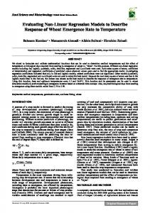
Assumptions of linear regressions (i.e homoscedasticity and normality of residuals) and lack of influential points were checked by drawing the standard ...
S2 Figs. Diagnostic plots of linear regression models. Assumptions of linear regressions (i.e homoscedasticity and normality of residuals) and lack of influential points were checked by drawing the standard diagnostic plots of R.
32
1
2
3
Normal Q-Q
-1 0 -3
16 141
Standardized residuals
0.0 -1.0 -2.0
Residuals
1.0
Residuals vs Fitted
3216 141
-1
0
1
2
Residuals vs Leverage
0.5
4.5 5.0 5.5 6.0 6.5 7.0 7.5 Fitted values
14 39
-1 0 1
32
-3
141 16
2 3
Scale-Location Standardized residuals
Theoretical Quantiles
1.0
1.5
-2
Fitted values
0.0
Standardized residuals
4.5 5.0 5.5 6.0 6.5 7.0 7.5
32 Cook's distance
0.00
0.02
0.04
0.5
0.06
Leverage
Figure S2.1: Diagnostic plots for log(APP abundance) vs. log(chlorophyll a concentration) fitted for all data.
Residuals vs Fitted
5.1
141
5.2
5.3
5.4
2 1 0 -3 -2 -1
Standardized residuals
0.5 -0.5
Residuals
-1.5
64 61
Normal Q-Q
5.5
64 61 141
-2
Fitted values
5.3
5.4
Fitted values
5.5
2
2 1 -1 0 -3
Standardized residuals
1.5 1.0 0.5
5.2
1
Residuals vs Leverage
141
0.0
Standardized residuals
5.1
0
Theoretical Quantiles
Scale-Location 61 64
-1
0.5
64
61 Cook's 141 distance
0.00
0.04
0.08
1
0.12
Leverage
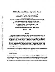
Figure S2.2: Diagnostic plots for log(APP abundance) vs. log(chlorophyll a concentration) fitted for data data points where organic matter free suspended solid concentration (TSS-Org) is below 50 mg/l.
32
1
2
37
0 -3 -2 -1
16
Normal Q-Q Standardized residuals
-1.0
0.0
37
-2.0
Residuals
1.0
Residuals vs Fitted
5.0 5.5 6.0 6.5 7.0 7.5
32
-2
Fitted values
0
1
2
5.0 5.5 6.0 6.5 7.0 7.5
Residuals vs Leverage 2
37
0
1
14
-3 -2 -1
Standardized residuals
1.5 1.0 0.5 0.0
Standardized residuals
32
37
Fitted values
-1
Theoretical Quantiles
Scale-Location 16
16
Cook's 32 distance 0.00
0.02
0.04
0.06
0.5
0.08
Leverage
Figure S2.3: Diagnostic plots for log(APP abundance) vs. log(chlorophyll a concentration) fitted for data data points where organic matter free suspended solid concentration (TSS-Org) is above 50 mg/l.
32
1
2
3
Normal Q-Q
-1 0 -3
16 141
Standardized residuals
0.0 -1.0 -2.0
Residuals
1.0
Residuals vs Fitted
3216 141
-1
0
1
2
Residuals vs Leverage
0.5
4.5 5.0 5.5 6.0 6.5 7.0 7.5 Fitted values
14 39
-1 0 1
32
-3
141 16
2 3
Scale-Location Standardized residuals
Theoretical Quantiles
1.0
1.5
-2
Fitted values
0.0
Standardized residuals
4.5 5.0 5.5 6.0 6.5 7.0 7.5
32 Cook's distance
0.00
0.02
0.04
0.5
0.06
Leverage
Figure S2.4: Diagnostic plots for log(APP contribution) vs. log(chlorophyll a concentration) fitted for all data.
64 61
0.8
1.0
1.2
1.4
0
1
2
83
-1 -2
Standardized residuals
0.0 0.5 1.0
Normal Q-Q
83
-1.0
Residuals
Residuals vs Fitted
1.6
61
-2
1.2
1.4
Fitted values
1.6
1
2
2 1 0 -1 -2
1.0 0.5
1.0
0
Residuals vs Leverage
61 64
Standardized residuals
1.5
Scale-Location
0.8
-1
Theoretical Quantiles
0.0
Standardized residuals
Fitted values
83
64
136
64 Cook's distance 61
0.00
0.04
0.08
0.5
0.12
Leverage
Figure S2.5: Diagnostic plots for log(APP contribution) vs. log(chlorophyll a concentration) fitted for data data points where organic matter free suspended solid concentration (TSS-Org) is below 50 mg/l.
Residuals vs Fitted
65 150
1.5
1.6
1.7
1 0 150
-2
-1
0
1
2
Theoretical Quantiles
Scale-Location
Residuals vs Leverage 2
0.5
0.5
1.5
1.6
1.7
Fitted values
1.8
1 0 -1
1.0
149
5
-2
65
0.5
65
Cook's distance 150
-3
Standardized residuals
1.5
149 65
Fitted values
150
1.4
-1
1.8
0.0
Standardized residuals
1.4
-2
149
-3
Standardized residuals
0.0 0.5 -1.0
Residuals
2
Normal Q-Q
0.00
0.05
0.10
1
0.15
Leverage
Figure S2.6: Diagnostic plots for log(APP contribution) vs. log(chlorophyll a concentration) fitted for data data points where organic matter free suspended solid concentration (TSS-Org) is between 50 and 500 mg/l.
1 0 -1 -2 -3
151 153148
Normal Q-Q Standardized residuals
0.0 -1.0
Residuals
0.5
Residuals vs Fitted
-1
0
1
2
Scale-Location
Residuals vs Leverage
Fitted values
1 0 -1 -2
0.5
1.5 1.6 1.7 1.8 1.9 2.0
3
0.5
-3
153148 151
Standardized residuals
Theoretical Quantiles
1.0
1.5
-2
Fitted values
0.0
Standardized residuals
1.5 1.6 1.7 1.8 1.9 2.0
151 148 153
148 distance Cook's 153
0.00
0.04
0.08
1
0.12
Leverage
Figure S2.7: Diagnostic plots for log(APP contribution) vs. log(chlorophyll a concentration) fitted for data data points where organic matter free suspended solid concentration (TSS-Org) is between 50 and 500 mg/l.