Sales and Consumer Demand for Storable Goods∗ Sofronis Clerides†
Pascal Courty‡
PRELIMINARY AND INCOMPLETE DRAFT PLEASE DO NOT CIRCULATE
May 6, 2010 Abstract A large literature has documented and proposed explanations for the large spike in sales of promoted grocery store items. Using a new dataset we set out to identify a broad set of stylized facts about sales promotions that can be observed in aggregate, store-level data. A promotion has an impact on sales of competing products as well as sales of the promoted product in future periods, but the magnitudes of these impacts are small relative to the increase in sales of the promoted product. We propose a simple model that can generate the aggregate patterns observed in the data. Consumers in the model are faced with regular and sale prices and are able to store at some cost. They differ in their willingness to engage in inventory management and in their degree of brand loyalty. The model does quite well in generating the aggregate patterns observed in the data and provides a useful tool for further analysis. Keywords: sales, promotions, market segmentation, consumer inventory, demand acceleration, stockpiling. JEL Classification: L12, L13, D4.
∗
We thank Machi Michalopoulou for excellent research assistance and Antonis Michis for invaluable help in understanding the data. We are solely responsible for any errors. † University of Cyprus and CEPR;
[email protected]. ‡ University of Victoria and CEPR;
[email protected].
1
1
Introduction
Temporary reductions in price are frequently observed in many retail markets. These events have drawn the attention of economists because the large price shifts and the associated movements in sales volumes provide a lot of variation that can be leveraged to analyze consumer behavior.1 Much of the interest has focused on frequently purchased items typically sold in grocery stores (detergents, food items, etc.). A stylized fact that has been widely documented is that temporary price reductions generate a very large spike in sales of the promoted product, often reaching several times the sales of the same product during non-promotion periods. The magnitude of the response to sales is difficult to reconcile with simple models of consumer choice and several explanations have been proposed. An obvious explanation is increased consumption: sales increase during promotions because consumers will consume more of a product when its price is lower. A second explanation is demand accumulation, the notion that consumers with low valuations accumulate as they wait around for a sale. Demand accumulation can be thought of as a special type of a consumption effect where increased consumption is due solely to new buyers. A third explanation is switching from other brands or retailers. This is the textbook story of static substitution: a lower price will induce consumers to switch from their usual brand or even to visit another retailer. A fourth explanation is consumer inventory management, which refers to the general notion that consumers shift purchases across time in order to take advantage of low prices during promotions. Several terms have been used in the literature to describe this behavior (demand acceleration, demand anticipation, stockpiling), but they all refer to the idea of consumers making purchases in order to store for future consumption rather than for current period consumption. Existing economic literature on promotions has provided evidence in support of some of these explanations. In a study of ketchup sales, Pesendorfer (2002) found that the increase in sales during a promotion is positively correlated with the time elapsed since the last promotion, which is interpreted as evidence of demand accumulation. Hendel and Nevo (2006b) use store and consumer level data to study consumer inventory behavior for laundry detergents, yoghurt and soft drinks. They provide several pieces of evidence that are consistent with demand anticipation. The same authors point out elsewhere that temporal effects – exemplified by the post-promotion 1
In the extensive marketing literature on this issue, temporary reductions in price are generally called “sales promotions” or simply “promotions”. The economic literature has predominantly used the term “sales”. This might cause some confusion as the term “sales” is generally used to describe price reductions of a more general nature, such as clearance sales (it also has the meaning of “quantities sold”, which adds to the confusion). The term “sales promotion” conveys more accurately the temporary nature of the phenomenon. In this paper we use the terms “sales” and “promotions” interchangeably.
1
dip, the drop in sales of a promoted product in the periods following the promotion – are relatively small in magnitude (Hendel and Nevo, 2003).2 This is consistent with the large marketing literature which has focused on tracing the sources of the sales increase and finds that it is mostly due to brand switching rather than to inventory behavior or consumption effects.3 In this paper we take a more holistic approach than the existing economic literature. Rather than focusing on developing and testing specific hypotheses, we set out to identify a comprehensive set of stylized facts about sales promotions that can be seen in aggregate, store-level data. With our findings as a guide, we then write down the simplest possible model that can generate the key patterns in the data. Our model allows us to give a fresh interpretation to existing findings and helps understand the consumer behavior that generates observed patterns. In our empirical analysis we use a new dataset on the laundry detergent market in the Netherlands. Laundry detergents are an appropriate choice for our purposes because consumption effects for this product are likely to be minimal. Consumers are not likely to do laundry more often because detergent is cheap. It is also hard to imagine that there are many consumers who make do without laundry detergent and only purchase it when the price is low. We can thus rule out consumption effects as possible explanations for the spike in sales during promotions. Our analysis of the data confirms the main findings of existing studies but also adds some new ones. Promoted items in our data experience a large spike in sales, by a factor of 5-10 depending on the product. There is evidence of a drop in sales of competing products but the impact is small. Even substitution across different size containers of the same physical product is surprisingly small.4 Consistent with existing literature, we find evidence of a post-promotion dip that is significant but relatively small in magnitude. Taken together, the estimated drop in sales of competing products and of the same product in future periods can only account for a small fraction of the increase in sales of the promoted product. The mass of new sales does not come from consumers who would have bought something else this period or from consumers who would have bought the item in adjacent periods. Where then do the extra sales come from? In order to answer this question we develop a simple model of demand for storable goods. We consider a good for which consumption is fixed; 2
We also note the important work of Erdem, Imai, and Keane (2003) and Hendel and Nevo (2006a), who develop structural models of consumer choice that focus on capturing consumer behavior in the face of stochastic price fluctuations. 3 See Blattberg, Briesch, and Fox (1995) and Neslin (2002) for useful surveys and van Heerde, Leeflang, and Wittink (2004) for more recent work. 4 This apparent puzzle is explored further in Clerides and Courty (2010).
2
consumers can not put off consumption for future periods. This is a reasonable assumption for detergents. There are two types of consumers. One segment are the passive consumers, who purchase a single unit of their preferred item whenever they run out of stock. Passive consumers do not engage in inventory management, possibly because of storage costs or time costs. A second segment consists of consumers who are actively engaged in inventory management. Active consumers have no brand loyalty and will take advantage of sales promotions whenever possible. Stockpiling is constrained by rapidly increasing storage costs. The model can generate the key aggregate patterns observed in the data. Sales of the promoted product increase because active consumers purchase to store and because they switch from other brands. Sales of other brands go down, as well as sales of the promoted product in future periods. The model can also deliver the prediction that the spike in sales is increasing in the time since the last promotion. Our model highlights a mechanism by which stylized facts about the demand response to promotions can be rationalized and it allows us to give a fresh interpretation to existing findings. The literature has emphasized the fact that most of new sales during promotions can be attributed to brand switching. This might reasonably lead someone to expect that sales of brand A in the current period will seriously suffer as consumers switch en masse to brand B. This is not the case; in our data, the impact of a promotion on contemporaneous sales of competing brands is surprisingly small. Our model provides a way out of this apparent contradiction. The increase in sales due to brand switching does not come at the expense of other brands because brand switchers do not have any brand allegiance to begin with. They are simply bargain-hunters who seek to always buy at the lowest price. In that sense the term brand switching is misleading in implicitly suggesting that people switch allegiances because of promotions.
2 2.1
Stylized facts about sales promotions Data description
Our analysis is based on a unique dataset from the laundry detergents market in the Netherlands. The data were obtained from ACNielsen and cover a period of 120 weeks between September 2002 to December 2004. We observe every size of every brand sold in each of the country’s four major chains, Albert Heijn, Super de Boer (formerly Laurus), Schuitema and Superunie. For each size we observe the total quantity sold and the sales-weighted average price. The detergent market is dominated by three multinationals (Henkel, Procter & Gamble, Unilever) but private labels also have a significant presence. Each manufacturer markets several brands and each brand name is carried by several products. 3
Table 1: Main manufacturer characteristics Manufacturer
Market share by: Sales Revenue
Firm 1 Firm 2 Firm 3 Firm 4 Private labels Other brands
.320 .290 .223 .032 .126 .009
Number of unique: Brands Products Sizes
.298 .312 .251 .037 .093 .009
Total
6 3 3 2
28 16 21 7 6 5
75 46 56 12 22 9
14
83
220
Sizes per product 1.55 1.81 1.61 1.29 2.33 1.45
Table 1 reports some key characteristics of each manufacturer as they appear in our dataset. We note the dominance of the three multinationals but also the significant presence of private labels. There a number of other manufacturers with a very small presence. Private labels are of course more than one firm; as a rule, each retail chain carries a single private label, usually its own. Each of the four manufacturers promotes several brand names and each brand name is carried by several products. The number of distinct packs produced by each manufacturer is quite large. Note however that not all sizes are available at all times. The last column gives the average number of sizes available to the consumer at a given point in time, which is a much smaller number than the number of sizes per product overall. Private labels stand out in having more sizes available than other manufacturers (2.33 sizes per product versus fewer than two for all others). A shortcoming of our data is that our information is at the level of the chain, not the individual store. The reported sales are aggregated over all stores and the price is a weighted average. A possible problem with this is that some items might not be available in all stores and thus will not be in the choice set of all consumers. Indeed the patterns we observe in the data suggest that this is likely to happen in the case of Superunie and probably also Schuitema. In order to be conservative we will limit our analysis to the Albert Heijn chain for which we are quite confident that the data are reliable. Albert Heijn carries only the major multinationals and its own private label. Its product lines are small – almost all products come in one or two sizes – and stable. Prices and sales also exhibit smooth and stable patterns. All of this is consistent with the assumption this retailer carries the same products is (almost) all of its stores. All data analysis in the remainder of the paper will thus focus solely on Albert Heijn. Figure 1 plots the temporal evolution of price and quantity sold for a selected product that is sold in the same two sizes every week throughout the period. The top part of the figure shows 4
Price
5
4
3
20
30
40
50
60
70
80
90
100
110
120
10
20
30
40
50
60 Week
70
80
90
100
110
120
3
ln(Quantity sold) 4 5 6 7 8
10
Small size
Large size
Figure 1: Price and sales path of a selected product the price per unit quantity of each size. Promotions are easy to identify in this plot as large and temporary downward deviations from the regular price. In each promotion the price drops sharply for a week, partially recovers in the following week and returns to its original level the week after that. Thus promotions last for between one and two weeks. In the first week all units are sold at the discounted price while in the second week some units are sold at the discounted price and others at the regular price, leading to a sales-weighted price lying somewhere between the two. The bottom graph in Figure 1 shows the sales of each pack on a logarithmic scale. The impact of promotions is quite striking, with a large spike in sales for the promoted pack. This is the main fact we seek to explain. In order to proceed we need to provide an operational definition of what constitutes a promotion. In the spirit of existing literature, we identify a promotion as a temporary decrease in price of at least 10%.5 In practice this is implemented by looking at a six-week window around any given price. If the price in the current period is at least 10% lower than the modal price during the six-week window, then the current period is labeled as a promotion period. Promo5
Some authors use a 5% threshold. We prefer to be more conservative on what constitutes a promotion.
5
Table 2: Descriptive statistics on promotions Total proms Firm Firm Firm Firm
1 2 3 4
152 105 101 32
Promotions per item Mean Median Max. 5.4 7.4 5.0 3.6
4 8 4 4
% time on prom. Mean Median
14 12 11 7
6.9 7.3 6.5 5.1
5.4 7.0 7.3 3.9
% prom. discount Mean Median 26.5 28.2 25.6 25.9
28.9 30.3 27.8 27.7
tions lasting more than one week are counted as one event. The use of the six-week window to define promotions means that we cannot identify promotions in the first and last three weeks of the data, leaving us with 114 weeks of data. This procedure identifies 390 promotions, the properties of which are summarized in Table 2. Firm 1 does the most promotions (152), but it also has the most products. Firm 2 is actually the most frequent promoter in relative terms as it averages 7.4 promotions per item and its products are on promotion 7.3% of the time on average. Firm 4 (the private label) is the least frequent promoter. The depth of discounts is in the range 25-30% and is very similar across firms. These price patterns are consistent with those reported in Hosken and Reiffen (2004). It is evident from Figure 1 that promotions of the particular product portrayed in the graph are associated with a very large increase in sales. This is true more generally. For every item, we calculated median sales during weeks when it is on promotion and during weeks when it is not promoted. The ratio of the two figures for the median product is a striking 12.6. In other words, a (median) discount of 29% multiplies sales by a factor of 12.6, implying an elasticity of about 40. With such a large impact on own sales, one would expect an impact on sales of competing products. Turning again to Figure 1, there appears to be a dip in the sales of the non-promoted pack during a promotion, but this is orders of magnitude smaller than the increase in sales of the promoted pack. The median drop in sales when an different size version of the same product is promoted is only 2%. Clearly the additional sales of the promoted product do not come from consumers switching from different packs of the same product but from other sources.
2.2
Contemporaneous effects
We use regression analysis to formally test several hypotheses about substitution patterns in the presence of promotions. We follow a reduced-form approach that links the (log) quantity sold of a particular item to whether there is currently a promotion of either the item itself or other
6
Table 3: Impact of sales by product type Premium brands Own promotion when no other size exists Own promotion of large size Own promotion of small size Promotion of smaller alternative Promotion of larger alternative Promotion of premium product Promotion of value product Obs. F-stat Item and brand-week fixed effects are included. Significance levels: † : 10%, ∗ : 5%, ∗∗ : 1%.
Value brands
2.171∗∗ (0.058) 2.151∗∗ (0.112) 2.378∗∗ (0.070) -0.109 (0.070) -0.027 (0.107) -0.043 (0.028) -0.069∗∗ (0.026)
1.605∗∗ (0.136) 0.496∗∗ (0.132) 2.060∗∗ (0.112) -0.532∗∗ (0.110) -0.129 (0.128) -0.078 (0.048) -0.001 (0.046)
3,846 19.50
1,982 8.57
items. The first specification aims to capture static substitution. The specification is based on our experience from other work with these data.6 We allow the impact of an own promotion to differ depending on whether the promoted item is competing with different sizes of the same product. The impact of a promotion of a competing size is allowed to differ depending on whether the promoted item is smaller or larger in size. The equation is estimated separately for premium and value brands.7 The specification includes pack size fixed effects, which control for the selection rule that determines which products are promoted. It also includes brand-week fixed effects, which control for marketing activities targeting specific brands. The results are presented in Table 3. The first three coefficients capture the impact of own promotion. They are all positive, large and highly significant. Premium brands get a larger boost from own promotions, probably because value brand buyers are more likely to switch to premium brands than premium brand buyers are to switch to value brands. The next two 6
Clerides and Courty (2010). Value brands are the private label plus Henkel’s Witte Reus and Unilever’s Sunil. The latter two brands sell at a substantial discount relative to other brands sold by the three multinationals. 7
7
8 6 Quantity sold 4 2 0 0
20
40
60 Week
80
100
120
Figure 2: Total category sales over time coefficients capture the impact of a promotion of a different size of the same product. The impact is essentially zero in the case of premium brands. For value brands the impact is quite substantial in the case of a promotion of a smaller alternative because this leads to an abritrage opportunity.8 The last two coefficients capture the impact of a promotion of a different product. All four coefficients are positive but the magnitudes are quite small and only one is statistically significant. These findings suggest that contemporaneous substitution across sizes and brands is limited and can not be the source of sales gains of the promoted product. As a final piece of evidence we look at aggregate weekly sales for all products in the laundry detergent category. If the increase in sales associated with promotions is the result of contemporaneous substitution then aggregate category sales should not be affected and total sales would be flat over time (especially given that consumption needs are to a large extent fixed). Figure 2 shows that this is not the case; there is large variation in sales over time. Turning to the data, we find that in weeks with at least one promotion category sales are 81% higher than in weeks with no promotions. We also estimated a regression of category sales on a set of dummy variables capturing the impact of an additional promotion. The estimates indicate that the first promotion increases category sales by 27% and additional promotions up to the fourth one increase sales further. Thus promotions expand category sales in the promotion period. In the next section we examine whether the expansion of sales comes at the expense of sales in periods before or after the promotion. 8
See Clerides and Courty (2010) for a detailed analysis of this issue.
8
2.3
Intertemporal effects
In this section we test hypotheses of an intertemporal nature, such as demand acceleration and the closely related idea of stockpiling. In order to clarify the implications of each hypothesis, consider a simple model where N consumers each purchase a single unit of a specific item every k weeks. Purchases by these consumers are evenly distributed over time, so N/k units are sold each week. Suppose that an unanticipated promotion is carried out in week t. If consumers are myopic, N/k units will be sold as usual. The hypothesis of demand acceleration suggests that consumers who were scheduled to purchase in weeks t + 1, t + 2, and on will may an incentive to accelerate their purchases in order to take advantage of the lower price, as long as the savings do not exceed their storage costs. Stockpiling differs from demand acceleration in a couple of ways. First, consumers who are scheduled to make a purchase at time t would not change their behavior under demand acceleration but they would under stockpiling. Second, consumers can potentially stockpile many units of the good while in the standard demand acceleration story they only move one purchase. It is important to note that expectations of future promotions severely limit the extent of acceleration and stockpiling. Consumers will not stock up if they expect the item to be on sale again in a few weeks. In order to test the extent of substitution over time we regress log sales on a set of dummies identifying periods before and after promotions. The results are displayed in graphical form in Figure 3. The solid line represents the estimates and the dotted lines delineate the 95% confidence interval. The interpretation of this graph is the same as the bottom graph in Figure 1, except that it displays the average impact of promotions after pack and brand-week fixed effects have been removed. Period 0 is the promotion period and we present five periods before and five periods after it. We include preceding periods in order to test for an anticipation effect: if consumers expect a promotion to take place in the next week or two, they might put off purchases until then. Evidence of an anticipation effect would suggest that consumers can predict promotion events quite accurately. There is little evidence of such anticipatory behavior except a marginally significant impact in period -3, which seems more like an anomaly rather than a part of any pattern. In week 0 we observe the expected impact of a promotion. The large positive impact observed in week 1 is the result of promotions spilling into a second week, so week 2 is really the first post-promotion week. We observe a statistically significant impact in weeks 2, 3 and 4, with all three coefficients in the range -0.08 and -0.09. The promotion impact vanishes by week 5. The estimates are consistent with a demand acceleration story. It should be noted, however, that the magnitude of the acceleration is small and can only account for a small fraction of the sales
9
2.5 2 1.5 1 .5
Impact on ln(sales)
0 −5
−4
−3
−2
−1
0
1
2
3
4
5
Period (promotion period = 0)
Figure 3: Estimated impact of a promotion across time increase in the promotion period. Consider the example above and suppose that a promotion leads to a 10% decrease in sales in the five weeks following it (which is larger than the effect we estimate). This level of acceleration leads to a ratio of sales during promotion to sales in the five post-promotion periods of only 1.67. Reproducing the 12.6 factor observed in the data would require 65.9% of consumers in each of the five periods to move their purchases forward. This fraction would have to be even larger if we were to divide promotional sales by the average of all non-promotion periods, which is the more correct measure. Our second specification mirrors the demand accumulation test implemented by Pesendorfer (2002). We allow the contemporaneous impact of a promotion on own sales to depend on the time elapsed since the same product was promoted. We find that the impact is increasing in the time but at a diminishing rate. This is consistent with demand accumulation though also with other explanations.
2.4
Summary of findings
The analysis in this section has produced a number of findings, some of which confirm existing findings while others are new contributions. As expected, sales promotions lead to a large increase in sales of the promoted product. In our data sales multiply by a factor of 5-10, depending on the product. Sales of competing products decrease but the impact is surprisingly small, especially when compared to the huge spike in sales of the promoted product. Put together, the two findings imply that category sales increase substantially in the period of the
10
promotion. We also find evidence of a post-promotion dip. Sales of the promoted product drop by a total of about 25% in the three weeks following the promotion, relative to regular sales. This is broadly consistent of other studies and can be interpreted as evidence of inventory management by consumers. Importantly, the lost sales during the post-promotion dip are only a small fraction of the sales increase during the promotion. Hence stockpiling and demand anticipation can only be part of the story.
3
A model of demand for fixed consumption goods
In this section we develop a model of demand for frequently purchased storable goods such as detergents. The objective is to replicate the aggregate patterns observed in the data: a very large response to own promotions but a small impact on competing items and a small degree of intertemporal substitution. The model could also apply to storable food items, such as rice. A key assumption is that a fixed quantity of the good is consumed every period. This is reasonable if the total expenditure on the good is relatively low and as long as prices stay within some “acceptable” range. The model also recognizes that goods are stored in containers of fixed size, hence quantity purchased is not a continuous variable.
3.1
Model description
The key ingredients of the model are the following: A1. Consumption. Consumers have fixed consumption needs of x per period (week). A2. Products. The good is sold in containers of size Q = kx, where k is an integer. Only one size is available. A3. Prices. There is a regular price pR for the good. In any period following a regular price, a sale price pS will be offered with probability π. Consecutive sales do not occur. That is, P r(pt = pS |pt−1 = pR ) = π and P r(pt = pS |pt−1 = pS ) = 0. The transition probability matrix is given in Table 4. A4. Storage. Storage costs are 0 for the first unit, φ for the second unit and ∞ for additional units. We assume that pR − pS > φ so that storage of a single unit is profitable.
11
Table 4: Transition probability matrix for prices pt−1 = pR pt−1 = pS
pt = pR
pt = pS
1−π 1
π 0
A5. Stock-outs. There is a cost χ of not being able to consume in a given period. We assume that χ is sufficiently high to rule out stock-outs. A6. Consumer types. There are N consumers. A fraction ω of consumers are passive. They follow a simple rule of purchasing a single unit when their stock reaches zero. This could be justified as high storage costs, high transaction costs or high costs of tracking prices. The remaining (1 − ω) fraction of consumers are active: their objective is to minimize the cost of ensuring that at least x is consumed every period. A7. Transaction costs. In principle one could add a transaction cost τ that would be incurred every time a consumer makes a purchase for this good and would be independent of the quantity purchased. This would represent the cost of adding the item to the list and locating it in the store. Having a transaction cost can help eliminate the possibility that consumers will buy a container of size x every period (if it is available). For now we just assume that this size does not exist and set τ = 0. Note that a transaction cost can explain storage independently of demand anticipation. A8. Timing. The consumer visits the store once in each period. At the beginning of every period the consumer observes his stock. He then goes to the store, observes prices and makes his purchase (if any). At the end of the period he consumes x. A storage cost is incurred during the period of purchase even if the good is consumed in the same period. Assumption A3 is meant to capture in a simple way the key features of the typical price process: there are usually two distinct prices, a regular price and a sale price, and sales are difficult to predict. We think it is natural to assume that, from the consumer’s perspective, sales are essentially random events. The state variable in this model is the quantity in stock at the beginning of the period, measured as number of containers. Hence the possible values of the stock variable will be multiples of x/Q = 1/k; that is, st ∈ {0, 1/k, 2/k, 3/k, . . .}. The highest value of the state variable at which a purchase will be made is st = 1 (otherwise the cost of storing a container will be incurred, which is assumed to be infinite). If a purchase is made at st = 1 the stock in
12
the next period will be st+1 = 2 − x/Q = 2 − 1/k, which is therefore the highest possible value of the state variable. For simplicity, in the rest of the exposition we normalize x = 1 and assume that Q/x = k = 2. These imply that Q = k = 2. This can be easily generalized.
3.2
Derivation of optimal policy
Passive consumers will always follow a policy of buying a single unit when their stock is depleted (st = 0), which means buying a container once every k = 2 weeks. Let n(s, p) represent the policy function specifying the optimal number of units to be purchased as a function of current stock and price. Optimal policy for passive consumers is ( n(s, p|π = 0) =
1 if
s=0
0 if
s>0
(1)
This is also the policy that would be followed by all consumers, active and passive, if there were no sales (π = 0). The rest of the analysis focuses on active consumers. The assumptions that k = 2 means that the state variable can take values st ∈ {0, 1/2, 1, 3/2}. Recall that the units are containers and one container equals two weeks’ consumption. In periods with a regular price (pt = pR ), the optimal policy is simply to make a purchase of one unit if st = 0, and to not make a purchase otherwise (the same policy followed by passive consumers at all times). Consider now the case of a sale price, pt = pS . There are four possible states to consider: – st = 0 The consumer must decide whether to purchase one or two units. If one unit is purchased, he will end up with st+1 = 1/2. If two units are purchased, he will end up with st+1 = 3/2. Given that there will be no sale at t + 1 (by assumption on the price process), he will not make a purchase at t + 1, meaning that at t + 2 he will have either st+2 = 0 (if he purchases one unit at t) or st+2 = 1 (if he purchases two units at t). Thus he must compare the difference in value Vt+2 (1) − Vt+2 (0) to the cost of purchasing the extra unit and carrying it in storage. The latter cost is pS + 2φ. To understand the difference V (1) − V (0), note that if st = 0 the consumer will necessarily purchase one unit at the prevailing price, which will bring his stock to 1. At that point 13
he will face the same choice as if he had started with st = 1. Thus the difference in value V (1) − V (0) is the expected price to be paid to get from st = 0 to st = 1, which is πpS + (1 − π)pR . The consumer will purchase a second unit if the benefit πpS + (1 − π)pR exceeds the cost pS + 2φ, or if πpS + (1 − π)pR > pS + 2φ ⇒ (1 − π)(pR − pS ) > 2φ ⇒ π < 1−
pR
2φ ≡π ¯ − pS
The consumer will purchase a second unit if the probability of a sale is small; if the storage cost is small; and if the difference between regular and sale price is large. – st = 1/2 Purchase one unit (otherwise will have to buy at t + 1 at pR ). – st = 1 Same problem as whether to buy a second unit when st = 0. Will purchase if π < π ¯. – st = 3/2 No purchase because storage cost of third unit is infinite. Table 5 summarizes active consumers’ policy function n(s, p). Note that if π > π ¯ , sales are sufficiently common relative to the storage cost that consumers will never purchase a second unit when they already have a full one in stock. Hence the state s = 1.5 will never reached. If π π ¯) pS
0 1/2 1 3/2
1 0 0 0
2 1 1 0
1 1 0 0
14
3.3
Aggregate implications
We now examine the model’s aggregate implications. Consider first the case when there are no sales (π = 0). In this case, all consumers follow the simple strategy given in expression (1) and the state variable only takes the values 0 or 1/2. Suppose that at time t the state variable is uniformly distributed within each consumer segment. That is, half of each type of consumer have stock 0 and the other half have stock 1/2. Consumers with st = 0 will make a purchase and end up with stock st+1 = 1/2. Consumers with st = 1/2 will not make a purchase and end up with st+1 = 0. Thus in the absence of sales consumer’s stock alternates between 0 and 1/2. In each period, the number of units sold is N/2. Now suppose a sale occurs when half of consumers are at st = 0 and half are at st = 1/2. Passive consumers will continue to operate according to (1) and will purchase a total of ωN/2 units. Active consumers will implement the optimal policy summarized in Table 5. Let us first examine the case π < π ¯ . Half of active consumers (those with st = 0) will purchase two units and the other half (those with st = 1/2) will purchase one unit. Total purchases by active consumers will be 3(1 − ω)(N/2), giving a total of (3 − 2ω)(N/2) units sold during the sale period. This is greater than regular period sales, which is N/2. For example, if the two consumer segments are of equal size (ω = 1/2), then sales during a promotion are double that of the previous period in the case π < π ¯. At t + 1, the period following the promotion, the price goes back to the regular price by assumption. Passive consumers will purchase ωN/2 units as always. Active consumers will only purchase if their stock has been depleted. But none of them will be in this situation because they all bought at least one unit in the previous period. Hence only the passive will purchase in the period following a promotion and total sales will amount to ωN/2, which is less than sales in the period before the promotion. The same will happen at t + 2 (if there is no promotion) because the stock will be at 1 and 1/2. At t + 3 the stock will be back where it was before the promotion and sales will return to normal levels. The post-promotion dip, defined as the drop in sales in the period after a promotion relative to regular sales, is (N/2 − ωN/2)/(N/2) = 1 − ω. Table 6 shows a numerical example for the case N = 1 and ω = 1/2. The table assumes that there is a sequence of regular prices up to t − 1, a promotion at time t, and a return to regular prices afterwards. Looking at the first row which represents the case π < π ¯ , we observe that sales in the period before the promotion are 0.5 and double during the promotion period. They drop to half the normal sales during the two periods after the promotion and return to normal in the third period. Consider now the case π > π ¯ , when sales are more frequent. When the sale occurs all active 15
consumers will purchase a single unit. Total sales will be (2 − ω)(N/2), less than in the case π π ¯ ) consumers will stockpile more and the post-promotion dip will last two periods. If sales are more frequent (π < π ¯ ) consumers will stockpile less and the post-promotion dip will last only one period. Table 6: Impact of a single promotion on aggregate sales
Case π < π ¯ Case π > π ¯
t−1 pR
t pS
t+1 pR
t+2 pR
t+3 pR
0.5 0.5
1 0.75
0.25 0.25
0.25 0.5
0.5 0.5
The model can also generate the tendency for the sales spike to be increasing in the time since last promotion. In the example in Table 6 (case π < π ¯ ), suppose there is a second promotion at time t + 2. The stock held by active consumers at that point will be 1 and 1/2 (half of consumers at each level). The policy function dictates that both will purchase a single unit, leading to total sales of 0.75. This is less than what is sold during the first promotion. The fact that the second promotion comes soon after the first one means that people will have higher stocks and will purchase less. Thus sales during promotions are increasing in the time elapsed since the last promotion. In this model we have a single brand, so everything we observe is due solely to the effects of inventory management; in particular, there is no brand switching. In the next subsection we introduce multiple brands in the model.
3.4
Multiple brands
Assume that there are J different brands. Passive consumers have brand preferences and are equally split between the brands. Active consumers do not have a brand preference. If prices are the same they will randomly choose one of the brands; if one is on sale they will all purchase that one. Each brand is equally likely to be promoted. The price process remains the same: in each period one brand will be promoted with probability π, unless there was a sale in the 16
previous period. The assumptions will generate a stream of constant sales to each brand (from passive consumers), plus some additional sales coming from active consumers which will vary depending on prices. Total sales in each period will be the same as in the single-brand case because consumption needs and the price process are the same. The difference is that purchases by active consumers will be directed to the promoted brand and this will have a profound impact on the aggregate patterns. Consider the case π < π ¯ and recall that passive consumers purchase ωN/2 in every period when a single brand is available. When J brands are available – and assuming that passive consumers will be equally split across brands – each brand will sell ωN/2J units. Similarly, the (1 − ω)N/2 units purchased by active consumers will be split among the J brands so that each brand sells (1 − ω)N/2J units. Total sales for each brand will be N/2J. When a sale occurs, passive consumers will go on as usual but active consumers will all switch to the promoted brand. The promoted brand will sell ωN/2J (to passive consumers) plus 3(1 − ω)(N/2) (to active consumers), for a total of (3 − 3ω + ω/J)(N/2). The non-promoted brand will sell the usual ωN/2J to passive consumers. We are interesting in replicating some of the aggregate magnitudes observed in the data. One of these is the factor by which sales of the promoted item increase relative to regular period sales. In our model (for the case π < π ¯ ) this is Promotion period sales (3 − 3ω + ω/J)(N/2) = = ω + 3J(1 − ω) Regular period sales N/2J
(2)
A second magnitude of interest is the fraction of sales that come from brand switching (as opposed to storage considerations). Brand switchers are consumers who bought a different brand the last time they made a purchase. Since consumers are equally split across brands, this means that a fraction (J − 1)/J are brand switchers. Finally, the post-promotion dip, defined as the drop in sales in the period following a promotion relative to regular sales can be easily calculated as 1−(ωN/2J)/(N/2J) = 1−ω. The post-promotion dip depends only on the fraction of passive consumers; in particular, it is independent of the number of brands. In the case π > π ¯ , promotion period sales are ωN/2J to passive consumers and (2 − ω)(N/2) to active consumers, for a total of (2 − 2ω + ω/J)(N/2). The factor by which sales of the
17
promoted item increase is Promotion period sales (2 − 2ω + ω/J)(N/2) = = ω + 2J(1 − ω). Regular period sales N/2J
(3)
This factor is smaller than what we found in the the case π > π ¯ in (2) as one would expect. When promotions are more frequent there is less of an incentive to store. The fraction of sales from brand switching and the post-promotion dip are independent of π. Table 7 replicates the example of Table 6 for the two-brand case. Brand 1 is promoted at t + 1. In the case π < π ¯ its sales increase by a factor of 3.5, substantially higher than the factor of 2 in the single brand case. In the case π > π ¯ the factor is 2.5 in the two-brand case and 1.5 in the single-brand case. In both cases the post-promotion dip is 50% and half of the increase in sales can be attributed to brand switching. Table 7: Impact of a single promotion on aggregate sales with two brands
Case π < π ¯
Brand 1 Brand 2 Total
t−1 (pR , pR )
t (pS , pR )
t+1 (pR , pR )
t+2 (pR , pR )
t+3 (pR , pR )
0.25 0.25 0.5
0.875 0.125 1
0.125 0.125 0.25
0.125 0.125 0.25
0.25 0.25 0.5
Factor of sales increase of promoted brand: 3.5 Fraction of sales from brand switching: 50% Post-promotion dip: 50% Case π > π ¯
Brand 1 Brand 2 Total
0.25 0.25 0.5
0.625 0.125 0.75
0.125 0.125 0.25
0.25 0.25 0.5
0.25 0.25 0.5
Factor of sales increase of promoted brand: 2.5 Fraction of sales from brand switching: 50% Post-promotion dip: 50%
3.5
Discussion
The simple model developed in this section does quite well in replicating some of the key patterns observed in aggregate data. It posits the existence of two consumer types. One type does not engage to inventory management (due to high costs of time or storage) and is brand loyal. The
18
second type has no brand loyalty and actively engages in inventory management. This simple structure can generate a large spike in sales during promotions and much smaller impacts on competing product sales and on next-period sales. The model can also generate the stylized fact that the sales spike is increasing in the time since last promotion, which is usually interpreted as evidence of demand accumulation. There is currently a tension in the model in that the both the sales spike and the postpromotion dip are decreasing in ω. This makes it difficult to match the observed magnitudes more precisely. This tension can be resolved by generalizing the model beyond the case k = 2. This is next on our agenda. The model can also be enriched by adding containers of different sizes.
4
Summary and conclusions
A stylized fact that has been widely documented is that temporary price reductions lead to very large increases in sales of the promoted products, often reaching several times the sales of the product during non-promotion periods. The magnitude of consumer response to sales is difficult to explain with simple models of consumer choice and several explanations have been proposed and empirically tested. Evidence in support of demand accumulation and stockpiling has been found. A key finding is that most of the sales increase comes from brand switching rather than from intertemporal considerations. The literature does not provide a clear picture of the kind of demand structure that underlies observed patterns. This paper aims to fill this gap. Using a new dataset we set out to identify a broad set of stylized facts about promotions. Consistent with existing literature, we find that promotions lead to a very large spike in sales of promoted products and to a much smaller decrease in the sales of the same products in future periods. But we also find that the impact on sales of competing products is very small, which seems to be at odds with the finding that most of the sales increase comes from brand switching. Taken together, the estimated drop in sales of competing products and of the same product in future periods can only account for a small fraction of the increase in sales of the promoted product. We argue that the evidence is consistent with the existence of two large market segments. Consumers in one segment typically buy the same product every time, and they do not stockpile or anticipate future demand. Consumers in the other segment have no brand loyalty and actively manage their inventory in order to minimize the cost of satisfying their consumption needs. The
19
model we develop can generate the key patterns in the data. It allows us to give a fresh interpretation to existing findings and helps provide a better understanding of consumer choice in the context of storable goods.
References Blattberg, R. C., R. Briesch, and E. J. Fox, 1995, “How Promotions Work,” Marketing Science, 14, G122–G130. Clerides, S., and P. Courty, 2010, “Sales, Quantity Surcharge and Consumer Inattention,” unpublished manuscript. Erdem, T., S. Imai, and M. P. Keane, 2003, “Brand and Quantity Choice Dynamics Under Price Uncertainty,” Quantitative Marketing and Economics, 1, 5–64. Hendel, I., and A. Nevo, 2003, “The Post-Promotion Dip Puzzle: What do the Data Have to Say?,” Quantitative Marketing and Economics, 1, 409–424. Hendel, I., and A. Nevo, 2006a, “Measuring the Implications of Sales and Consumer Inventory Behavior,” Econometrica, 74, 1637–1673. Hendel, I., and A. Nevo, 2006b, “Sales and Consumer Inventory,” RAND Journal of Economics, 37, 543–561. Hosken, D., and D. Reiffen, 2004, “Patterns of Retail Price Variation,” RAND Journal of Economics, 35, 128–146. Neslin, S. A., 2002, “Sales Promotion,” in Barton Weitz, and Robin Wensley (ed.), Handbook of Marketing, SAGE Publications. Pesendorfer, M., 2002, “Retail Sales: A Study of Pricing Behavior in Supermarkets,” Journal of Business, 75, 33–66. van Heerde, H. J., P. S. J. Leeflang, and D. R. Wittink, 2004, “Decomposing the Sales Promotion Bump with Store Data,” Marketing Science, 23, 317–334.
20