Saliency Density Maximization for Efficient Visual Objects Discovery

IEEE TRANSACTIONS ON CIRCUITS AND SYSTEMS FOR VIDEO TECHNOLOGY, VOL. X, NO. X, XX XXXX

1

Saliency Density Maximization for Efficient Visual Objects Discovery Ye Luo, Junsong Yuan, Member, IEEE, Ping Xue, Senior Member, IEEE, and Qi Tian Senior Member, IEEE,

Abstract—Detection of salient objects in an image remains a challenging problem despite extensive studies in visual saliency, as the generated saliency map is usually noisy and incomplete. In this paper, we propose a new method to discover the salient object without prior knowledge on its shape and size. By searching the sub-image, i.e., a bounding box of maximum saliency density, the new formulation can automatically crop the salient objects of various sizes in spite of the cluttered background, and is capable to handle different types of saliency maps. A global optimal solution is obtained by the proposed density-based branch-andbound search. The proposed method can apply to both images and videos. Experimental results on a public dataset of five thousand images show that our unsupervised detection approach is comparable to the state-of-the-art learning based methods. Promising results are also observed in the salient object detection for videos with a good potential in video retargeting. Index Terms—Unsupervised salient object detection, Branchand-Bound search, maximum saliency density.

I. I NTRODUCTION HE STUDIES of psychology and cognitive science have shown that the human perception is attentional and selective [41]. For example, when watching images or videos, not every pixel is of equal importance to us. In most cases, our visual attention mainly focuses on a salient sub-region of an image, e.g. the salient object, and we follow this salient object in an image sequence. It is thus of great interests to discover the salient object and there have been many applications in image/video compression [2], [17], object tracking [5], retargeting [25], [4], [10], collage [27], [10] and object detection [29], object recognition [8], [7], [9]. In visual saliency studies, a lot of work have been focused on generating the saliency map of an image or a video frame [14], [3], [43], [26], [40], [1], [36], [45], [30], where the intensity of the map indicates how salient each pixel is. Although different saliency models have been generated, accurate detection of the salient object in a saliency map remains a challenging problem. It is not uncommon that the obtained saliency map is noisy and incomplete. As an example shown in Fig. 1, only several salient parts of the flower are highlighted in the saliency map, while the rest are missing. Due to the distraction from the cluttered background, it is not easy to accurately locate the salient object and crop it out. To handle this problem, some existing methods generate saliency maps by supervised learning methods and find the minimum rectangular region that covers a fixed amount of salient points, e.g. 95 % of the total salient points [26], [19]. The major limitation is that it is troublesome to train the model or difficult to predefine the amount of saliency the salient object should contain, as it depends on the size and the shape

T

of the salient object, as well as how cluttered the background is. Such a detection method thus cannot be adapted to various sizes of the salient objects. Instead of cropping the salient object with a bounding box, some other methods rely on object segmentation to obtain an accurate object shape. This category of methods, however, is not robust to the cluttered background and usually requries prior knowledge to help an accurate segmentation [1], [40]. To address the above mentioned problems, we propose a novel unsupervised method to discover salient objects from various saliency maps of images or videos. Given a saliency map of spatial size m × n, our goal is to detect a sub-image of smaller size m′ × n′ that well covers the salient object. To enable a robust detection, given the saliency map of an image, we propose to locate the object by finding a bounding box of the maximum saliency density (MSD). As a new formulation of salient object detection, it balances the size of the object and the saliency it should contain, thus can be adapted to the various sizes of the salient object. Moreover, it can tolerate the noise and incompleteness in the saliency map due to the cluttered background and the imperfectness of the saliency map. For example, as shown in Fig. 1, even though the salient pixels distribute sparsely, the detected bounding box with the highest saliency density accurately crops the salient object out. The proposed method does not require any prior knowledge of the salient object and is an unsupervised method. To avoid an exhaustive search of all possible bounding boxes, a branch-and-bound search algorithm is proposed to efficiently find the optimal one with maximum density rather than largest classification score [21]. Experimental results on a public dataset of five thousand images show that the performance of our salient object discovery is comparable to the state-of-the-art learning based salient object detection. The testing on four different types of saliency maps ( [3], [14], [1] and a fused saliency map ) show our method can perform equally well.

Fig. 1. Our salient object detection result using the saliency map proposed in [14]. The first image is the original saliency map. The second image is the binarized saliency map. The third image is the result of salient object localized by maximum saliency region detection. The red rectangle is the detected result while the blue one is the ground-truth from [26]. The last one is our result via saliency density maximization.

IEEE TRANSACTIONS ON CIRCUITS AND SYSTEMS FOR VIDEO TECHNOLOGY, VOL. X, NO. X, XX XXXX

Besides object detection in images, the proposed method can be easily extended to salient object detection in videos as well. The main difference between salient object detection in images and videos is that the salient object may move in videos. Given a sequence of saliency maps for a video shot, instead of identifying the salient object at each frame, we search for a sub-image region which covers not only salient objects of the current frame but also its previous peers’. Therefore, the detected sub-image contains most of the saliency of the video shot and keeps the temporal smoothness of the selected regions. We define the sub-image as the salient object for a video shot, which has the maximum saliency density on the global saliency map (name as importance map Imap , see Section 4A for more details) of all the frames. With this definition and detection method for video salient objects, the obtained sub-image can be cropped and applied to video retargeting. Such a cropping-based video retargeting does not distort the salient objects as seam carving, or introduce dithering under complex camera motions as in [4], [31]. The evaluations on a few video shots show that the proposed method extended in videos provides promising results even on challenging videos with dynamic and complex camera motions. Our major contribution is two-fold: 1) We first formulate the task of the unsupervised salient object detection as the maximum saliency density discovery problem, which well balance the size of the saliency object and the saliency it contains. It is also compatible to different types of saliency maps or a fused saliency map. 2) To obtain the global optimal solution of the saliency density maximization problem, we propose an efficient branch-and-bound search algorithm, which is based on the saliency density rather than the traditional classification scores. Derivation of the upper-bound estimation and the average convergent time (referred to table II) show its efficiency on salient object detection in both images and videos. The rest of paper is arranged as follows. Section II gives an overview of the related work. Section III and IV present our new salient object detection method for images and videos, respectively. The experimental results and discussion are given in Section V and Section VI. We conclude in Section VII. II. R ELATED W ORK During last two decades, visual saliency detection and saliency map generation aiming to find out what attracts humans’ attention got broad interesting in computer vision especially for object detection/recognition from different scenes. Based on the methods to generate saliency maps, there are two categories of computational models for saliency map generation: the edge/corner based method [14], [3], [43] and the global region based method [26], [40], [1], [30]. Global region based methods, e.g. Achanta’s method [1], generate larger visually consistent object regions than edge/corner based methods, e.g. in [14], [3]. In this paper, saliency map generation is not our focus. Instead, our interest is to discover salient objects from various saliency maps.

2

A. Salient Object Detection in Images Given the saliency map, the simplest way to obtain the salient object is by thresholding the saliency map to get a binary mask. Methods to threshold saliency map are intensively discussed in [24], [1], [15], [11], [19]. These methods depend on the selection of the threshold. In order to accurately detect salient objects from saliency maps, image segmentation is combined with the saliency map in [43], [40], [1]. However, the performance heavily relies on the accuracy of image segmentation results. Some heuristic methods [13], [20] are proposed to improve the performance of salient object detection. However, accurate detection of the salient object boundary is not always necessary. The other category of salient object detection is performed by finding the bounding box of the object. For example, a fuzzy growing algorithm to locate the attended area is proposed in [33]. Exhaustive search is adopted in [26] to find the smallest rectangle containing at least 95% of salient pixels for a learned saliency map model. Liu et al. [24] noticed the disadvantages of exhaustive search and proposed to use the dynamic threshold and the greedy algorithm to improve the search efficiency. However, their methods still rely on thresholds. In [40], the search of the rectangular sub-window is speeded up by applying the efficient sub-window search (ESS). ESS is a recently proposed branch-and-bound search algorithm for sliding window search on object recognition [21]. Salient object detection with bounding boxes has many applications in image analysis, such displaying images on a small device, or browsing image collection [40], [24], [34]. B. Salient Object Detection in Videos Salient object detected in videos can be performed by finding a rectangle bounding box in individual frame like the ways in images [6], [29]. In [29], a single salient object is detected by energy minimization and labeled by a bounding box in each frame. However, salient objects on consecutive frames are probably detected with different sizes, thus they cannot be simply cropped out and applied for displaying purpose. In order to consistently present the regions of interest detected from videos, an active window allowing slight orientation change is optimized in each frame to contain most informative pixels [39]. Liu et al. [25] found out salient regions from videos by minimizing penalties of information loss. Deselaers et al. [4] presented a supervised learning method to crop sub-windows based on the manually labeled salient regions. Both [25] and [4] have limitations due to virtual camera motions. The principled solution proposed in [16] allows the salient region of different sizes and considers the motion smoothness of the consecutive frames. However, it still has the risk of introducing virtual camera motions. To overcome limitations of these methods, we aim to automatically detect a global salient sub-image for a whole video, which optimizes the performance by preserving most of saliency and is robust on keeping the time coherence of selected regions. III. S ALIENT O BJECT D ETECTED IN I MAGES Given a single image I and its associated saliency map S, where S(x, y) indicates the saliency value of the pixel at

IEEE TRANSACTIONS ON CIRCUITS AND SYSTEMS FOR VIDEO TECHNOLOGY, VOL. X, NO. X, XX XXXX

3

(x, y), our goal is to accurately locate the salient object, i.e. to locate a salient sub-image W ⊆ I with maximum saliency density. We first review some existing methods, then propose our new approach. (a)

(b)

(c)

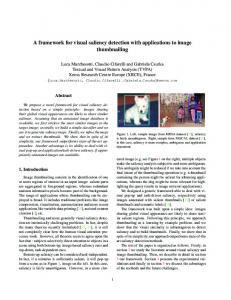
Fig. 2. (a) Original image (b) Sparse saliency map by [14] which highlights edges and corners (c) Dense saliency map by [1] which highlights overall salient regions.

A. Existing Schemes 1) Minimum Rectangle with Fixed Saliency (MRFS): Previous approaches treated a salient object as a smallest rectangle containing at least a fixed percentage of salient pixels (e.g. 95 %) from saliency maps [24], [1] or binary saliency maps [26] and the rectangle is obtained by exhaustively searching. As in [26], the binary saliency map is adopted and the formulation of salient object detection by MRFS can be written as in Eq. (1): W ∗ = arg min A(h(W )) W ⊆I P (x,y)∈W Sb (x, y) ≥ λ}, h(W ) = {W | P (x,y)∈I Sb (x, y)

(1)

where A(h(W )) measures the area size of h(W ) and Sb is the binary image of S. We set Sb (x, y) to 1 when S(x, y) ≥ τ and Sb (x, y) to 0 when S(x, y) < τ . Here, τ is the threshold; W is the sub-window of the whole image region I and λ is the fixed percentage. The brute force method works, however, it is not time efficient and λ is heuristically decided. 2) Maximum Saliency Region (MSR): Other approaches proposed that salient object detection can be solved as object localization by an efficient sub-window search [40]. Pixels on saliency map are scored by a binary classifier (salient and non-salient) and the salient object is the sub-window with maximum classification score. Based on the maximum subarray problem [21], [23], the sub-window can be found by an efficient sub-window search. Therefore, the idea of salient object detection in [40] can be formulated as in Eq. (2): W ∗ = arg max h(W ) W ⊆I X h(W ) = Sb (x, y),

(2)

1) Maximum Saliency Density: Since different saliency map generation methods emphasize different aspects, the obtained saliency map could be sparse or dense, as shown in Fig. 2. Sparse saliency map accurately detects the salient parts of the object but the boundary of the salient object is not well defined. Dense saliency map represents the salient object completely but some cluttered background is also included in the detection result. Despite different types of saliency maps, we notice that the average density of the region of salient object is much larger than that of any other regions on the saliency map. This motivates us to propose the salient object detection with maximum saliency density from the raw saliency map S. As a result, there is no need to select the threshold τ and the fraction ratio λ. Moreover, it balances the size of the salient object when the saliency map is sparse. To handle different types of saliency maps, we formulate our objective function f (W ) as: P P (x,y)∈W S(x, y) (x,y)∈W S(x, y) P . (3) f (W ) = + C + A(W ) (x,y)∈I S(x, y)

Here C is a positive constant to balance A(W ) which is the area of (W ). The first term in f (W ) prefers that W contains more salient points, while the second term ensures that the detected region W is of high quality in terms of the saliency density. Therefore, by finding the optimal bounding box W ∗ that maximizing the two terms together in f (W ) as in Eq. (4), we balance the size of the salient object and the saliency it contains. We call our new formulation as the maximum saliency density (MSD). W ∗ = arg max f (W ).

Sb (x,y)∈W

where Sb (x, y) is obtained in a similar way in Eq. (1) with a slight difference that Sb (x, y) = −1 when S(x, y) < τ . From Eq. (2), the salient object is located with the region W ∗ that contains the maximum of saliency. We call this method as the maximum saliency region. However, there are two major limitations of this method: (1) it highly relies on the selection of threshold τ , which is difficult to optimize; (2) when the binary saliency map is sparse, it intends to detect a small region.

B. Our New Approach Different from aforementioned methods, we present our new formulation and solution for the salient object discovery problem in this Section.

(4)

W ⊆I

2) Constrained Maximum Saliency Density: Depending on applications, we would have prior knowledge or requirement on the aspect ratio or the size of the salient object. For example, video retargeting requires the selected region has the same aspect ratio as the target display, to avoid visual distortion. Therefore, we further present an aspect ratio preserved solution to find the global optimal W ∗ . W ∗ = arg maxf (W ) W ⊆I P P S(x, y) (x,y)∈W S(x, y) (x,y)∈W , + f (W ) = P C + A(W ) (x,y)∈I S(x, y) s.t.

(5)

r0 − ∆r ≤ r ≤ r0 + ∆r

where r0 is the target aspect ratio and r is the aspect ratio of region W . ∆r is an offset allowed r to deviate slightly from

IEEE TRANSACTIONS ON CIRCUITS AND SYSTEMS FOR VIDEO TECHNOLOGY, VOL. X, NO. X, XX XXXX

r0 . This is based on the assumption that we allow slightly distortion if important information can be included in the detected region. 3) Detection Algorithm: Exhaustive search of W ∗ from either Eq. (4) or Eq. (5) is time consuming. W ∗ = [T, B, L, R] contains four parameters, where T , B, L, R are the top, bottom, left, and right positions of W ∗ , respectively. Suppose the frame is of size m × n, the original hypotheses space is [0, n − 1] × [0, n − 1] × [0, m − 1] × [0, m − 1], where we need to pick up T , B, L, R from each dimension respectively. To solve this combinatorial optimization problem, an exhaustive search is of complexity O(m2 n2 ). A branchand-bound search method is proposed in [21] to accelerate the search by recursively partitioning the parameter space and pruning the sub-space based on the calculated upper bound until it reaches the optimal solution. Such a branch-and-bound search can lead to the exact solution as the exhaustive search, while with a practical complexity of only O(mn). The details of the branch-and-bound search can be found in [21]. Despite its efficiency, the original branch-and-bound only works with both positive and negative values. However, in our case, the saliency map only contains positive elements and we do not want to deliberately introduce negative pixels. Therefore we need to develop our own branch-and-bound search algorithm. Considering the efficiency of the branch-and-bound searching method depends on the upper bound estimation, we derive the upper bound of our f (W ) first. Denote the set of regions by W = {W1 , . . . , Wi }, where each Wi ⊆ I. Suppose there exists two regions Wmin (Wmin ∈ W) and Wmax (Wmax ∈ W), such that for any (W ∈ W), Wmin ⊆ W ⊆ Wmax . Given the set W, we denote by fˆ(W) the upper bound estimation of the best solution that can be found from W. In other words, we have fˆ(W) ≥ f (W ), ∀W ∈ W, using Wmin and Wmax , the upper bound of Eq. (4) can be estimated as: P P (x,y)∈Wmax S(x, y) (x,y)∈Wmax S(x, y) ˆ f (W) = P . (6) + C + Area(Wmin ) (x,y)∈I S(x, y) As a similar scenario, the upper bound for Eq. (5) is derived as Eq. (7). Mathematical notations here follow Eq. (6). P P (x,y)∈Wmax S(x, y) (x,y)∈Wmax S(x, y) ˆ P f (W) = + , C + A(Wmin ) (x,y)∈S (x, y) (7) s.t. rmin − ∆r ≤ r0 ≤ rmax + ∆r

where rmin = W idth(Wmin )/Height(Wmax ) and rmax = W idth(Wmax )/Height(Wmin ). The expected aspect ratio r0 for region W ∗ is also bounded by Wmin and Wmax . Thus, f (W ∗ ) is the optimal solution according to the set W. Based on the upper bound estimation, our salient object detection algorithm is proposed. Here, only the constrained MSD salient object detection algorithm is given and shown in algorithm 1. Detection procedure without constraint is easily obtained by removing the if sentences in the algorithm. IV. S ALIENT O BJECTS D ETECTION IN V IDEOS To detect salient objects in videos, videos are first separated into shots with the consideration that salient objects are mov-

4

Algorithm 1: Aspect Ratio Constrained MSD Salient Object Detection Algorithm Data: Image saliency map S ⊆ Rm×n and upper-bound function fˆ(W) as Eq. (7) Result: W ∗ = arg max f (W ) W ⊆S

begin Set P as an empty priority queue W ← [0, n − 1] × [0, n − 1] × [0, m − 1] × [0, m − 1] while W contains multiple windows do W1 ∪ W2 ← W and W1 ∩ W2 = ∅ for i ← 1 to 2 do Find Wimin and Wimax from Wi Calculate rmin and rmax for Wi if (rmin − ∆r ≤ r0 ≤ rmax + ∆r) then Push (Wi ,fˆ (Wi ) into P Retrieve the top state W from P

ing smoothly within a shot. Given a video shot {I1 , · · · , It } (t is the frame number of the video shot), its corresponding saliency map sequence {S1 , · · · , St } is extracted. After getting the spatio-temporal saliency map, three steps are taken to detect a salient sub-image W across all frames. Firstly, salient object is obtained by MSD salient object detection algorithm at each frame. An importance map is then constructed by the frame salient object and the global optimal salient subimage for a video shot is finally obtained by searching on the importance map. A. Method Procedure 1) Spatio-temporal Saliency Map Extraction: The spatiotemporal saliency map S(x, y, t) for the frame It is defined as the weighted linear combination of the spatial saliency map SI and the temporal saliency map SM : S(x, y, t) = (1 − ω) × SI (x, y, t) + ω × SM (x, y, t),

(8)

where SI is the spatial saliency map proposed in [1] and SM is the frame difference to characterize the motion saliency. Here, ω ∈ [0, 1] is the weight to balance two terms and we set ω = 0.8 to emphasize the motion saliency. Based on the assumption that the fixation of humans is always in the image center, fused saliency map is weighted by a near flat Gaussian G(x − x0 , y − y0 , σ 2 ) as the attention priori: (x − x0 )2 + (y − y0 )2 ). (9) 2σ 2 Here, σ 2 is taken larger enough to make the priori value decay slowly when it approaches the frame boundary. (x0 , y0 ) is the image center. Semantic features such as face [44], [32], visual concepts [37] could also be added to improve the saliency detection. 2) Salient Object Detected in Each Frame: For each frame, a salient object Wt∗ is obtained by employing our maximum saliency density (MSD) salient object detection algorithm. Without any constraints, the result Wt∗ tightly bounds the S(x, y, t) = S(x, y, t) × exp(−

IEEE TRANSACTIONS ON CIRCUITS AND SYSTEMS FOR VIDEO TECHNOLOGY, VOL. X, NO. X, XX XXXX

5

Fig. 3. The first row: sampled saliency maps of tennis video clip; The second row: corresponding detected bounding boxes for frame salient object in green and the human labeled ground truth in blue; The third row: intermediate states of constructing Imap ; The last row: the global bounding box with the target aspect ratio r0 = 9/16 in red and the human labeled global ground-truth in blue.

salient object for the current frame. Moreover, by detecting Wt∗ , visual saliency caused by cluttered background is partially removed in each frame. It thus helps the global salient object detection in the video shot. 3) Importance Map and Globally Optimal Salient Subimage: Salient object Wt∗ detected in each frame cannot be treated as the final cropped region for each frame, as it does not incorporate any motion smoothness among different Wt∗ . Here, Wt∗ is actually a local optimal solution, which labels the salient object in an individual frame It . For a video shot, a global optimal W ∗ is related to Wt∗ but different from Wt∗ . To find the importance for other points with regard to the whole video shot, we generate an importance map Imap based on the frequency of a point S(x, y, t) falling into Wt∗ . The large value of Imap (x, y) indicates that the point (x, y) attracts our attention in the whole video sequence frequently. Hence, Imap serves as a mean filter to filter out outlier salient points that only appear in a few frames while not significant for the whole video: 1X Imap (x, y) = g(S(x, y, t)) (10) N t  1 S(x, y, t) ∈ Wt∗ g(S(x, y, t)) = 0 S(x, y, t) ∈ / Wt∗ . Here N is the total number of frames and normalizes all values in the important map into [0, 1]. The constrained MSD algorithm as described in algorithm 1 is used to search W ∗ in Imap which is the globally optimal salient sub-image for a video shot. B. Simulation on a Simple Video Shot with Human Labeled Ground-truth Due to lack of the ground-truth for salient object detection from videos, it is difficult to measure the efficiency of the proposed method quantitatively. We manually labeled a simple tennis video shot and simulate our method on it to better illustrate our ideas and the efficiency on salient object detection in videos. In the tennis video clip, the player is the

dominant and salient object while the ball and the shadow of the player are neglected because of either the small size or low contrast. Our aims here are two folds: detect the player per frame and select the best region to represent the whole video. In each frame, the ground-truth of the frame salient object is the blue bounding box of the player shown in the second row of Fig. 3. Since the player is moving within a limited range, the best region selected for displaying the whole video is the largest place the salient object can reach. This region is set to be the ground-truth of the global salient object detection. However, there is no aspect ratio constraint to this global ground-truth because it is barely based on the motion range of the salient object. When the target screen has aspect ratio constraint different from the largest place the salient object can reach, the size of the global ground-truth should be adjusted. To fairly and easily compare, we choose ∆r = 0 and r0 = 9/16 which is close to the aspect ratio of the ground-truth and no further adjustment is needed. Sample frames and their corresponding detection results are shown in Fig. 3. The sampled saliency maps in the first row of Fig. 3 show that the player keeps changing its shape and position as it moves. The green bounding boxes in the second row of Fig. 3 are our object detection results in single frame, which are compared to the blue rectangles (ground-truth of frame salient objects). That further validates that MSD method can adaptively detect the salient object regardless of its shape and position changes. The red bounding boxes in the third row of Fig. 3 are our global salient sub-image detection results constrained with aspect ratio 9/16. We can see that our results are close to the ground-truth with the assigned aspect ratio. The slight difference is because the predefined region is the largest region the salient object can reach while our method is to detect the region the salient object frequently appears. Specifically, given the binary mask of our detected region Sd in red and the ground-truth binary mask Sg in blue, we calculate

IEEE TRANSACTIONS ON CIRCUITS AND SYSTEMS FOR VIDEO TECHNOLOGY, VOL. X, NO. X, XX XXXX

precision and recall as in Eq. (11): P P S × Sd S × Sd Pg Pg precision = , recall = Sd Sg (1 + α) × precision × recall , F − measure = α × precision + recall

(11)

where α is a positive constant which weights the precision over recall while calculates F-measure. We take α = 0.5 as suggested in [40], [26]. TABLE I P RECISION , RECALL AND F- MEASURE FOR FRAME SALIENT OBJECT AND GLOBAL SALIENT SUB - IMAGE DETECTION IN TENNIS VIDEO CLIP. r0 = 9 : 16 precision recall F − measure

F rame 73.69% 93.36% 79.26%

Global 82.30% 86.67% 83.71%

The performance on precision, recall and F-measure for our method in the tennis video is given in table I, from which we can see our detection method can correctly locate the salient object either in a single frame or in a video shot. V. E XPERIMENTAL R ESULTS A. Salient Object Detection in Images 1) Database: In order to evaluate the results, the benchmark dataset in [26] is used to test our algorithm. The dataset provides 5000 images with the average spatial resolution of 300 × 400 or 400 × 300. Each image contains a salient object and each salient object is labeled by nine users by drawing a bounding box around it. Since different users have different preference of saliency, only the point voted more than four times is considered as the salient point. The averaged saliency map Sg is then obtained from the user annotation. To obtain the better performance of each saliency model especially for those sensitive to the image scales, we resize all the images and its corresponding ground truth masks into 3/4 of the original size. That means the spatial resolution of all images is set to m × n = 225 × 300 or m × n = 300 × 225. 2) Comparison of MSD with MRFS: First of all, we compare the proposed MSD with minimum rectangle with fixed saliency (MRFS). The parameter λ is set to 95% as [26] suggested. Fig. 4 shows the results obtained by MRFS and our method in the second and the last rows, respectively. As 95% is a fixed parameter and not determined by the content of the saliency map, only parts of the salient object are detected on Hou’s saliency map. It is mainly because most of salient points are the boundaries of the salient object in [14]. On contrary, the detected results of MRFS include a large part of the nonsalient object area on Achanta’s and Bruce’s saliency maps. While in our method, more salient object area is included owing to the first term in Eq. (3) on Hou’s saliency map, and small salient area away from main salient object is dropped under the constraint of the saliency density on Achanta’s and Bruce’s saliency maps. Therefore, our result is more accurate than MRFS. Precision, recall and F-measure on Fig. 5 further validate our claim. In order to evaluate λ, we test four different

6

λ values as Fig. 6 shows. Precision is improved while recall is reduced as λ becomes smaller and it is difficult to choose an optimal λ. 3) Comparison of MSD with MSR: To compare MSD with MSR, we test both methods on three different saliency maps. The threshold τ is obtained by Otsu [35] for all saliency maps in MSR. The parameter C is set to be 0.9, 0.03 and 0.24 of the size of m × n for Hou’s, Bruce’s and Achanta’s saliency maps respectively in MSD through parameter evaluation. Fig. 5 shows the comparison results. The average of precision, recall and F-measure are reported on each group. On Hou’s saliency map, edges/corners are detected as salient parts. By using MSR, very small region is bounded while larger salient regions are detected by MSD. F-measure and recall are significantly improved by MSD. For the other two saliency maps, MSD also outperforms MSR. The results on three different types of saliency maps show that MSD improves F-measure, and at the same time, keeps the high precision rate. 4) Evaluation on Different Saliency Maps: Since the salient object detection result is based on the saliency map, the more accurate the saliency detection is, the better performance the object detection method obtains. It is worth noting that a single salient object in [26] is obtained through supervised learning. Both [43] and [40] have prior knowledge about the region size provided by image segmentation. Thus, they are not directly comparable with the proposed method. However, even without any prior knowledge of the salient object, MSD on Bruce’s saliency map outperforms Ma’s method [33] which directly uses detected salient object (F-measure 61%) and search result on Itti’s saliency map [18] which finds the minimum rectangle containing at least 95% salient points by the exhaustive search (F-measure 69%). For MSD on Hou’s saliency map, it obtains comparable result compared with the exhaustive search on Itti’s saliency map. Though our result on Achanta’s saliency map is not as good as the result on [18], the precision is still higher than searching result on Itti’s and Ma’s saliency maps. Various saliency maps estimation methods are proposed recently. Evaluating the efficiency of them itself is an interesting problem. A small range comparison is performed in the paper as shown in Fig. 7. Since different bottom-up saliency map generation method has different advantages and disadvantages, to minimize the influence to the saliency object detection result, four saliency maps from [3], [14], [15], [1] are fused together. Each saliency map is normalized into [0, 1] and the combined saliency map is obtained by integrating them together, then normalizing the summation into [0, 1]. Different weights are tested and the ratio 2 : 1 : 1 : 2 for saliency maps [3], [14], [15], [1] respectively, which gets the best performance, is selected. As shown in Fig. 7 for our method 6, after combining four saliency maps together, F-measure is further improved to 75.84% compared to the best individual saliency map result from Bruce’s saliency map 73.06%. The performance is close to the learning based salient object detection results in [26] which requires training and has much higher computation cost. 5) Parameter Evaluation: Two groups of experiments are performed to evaluate the influence of the only parameter C in the proposed method.

IEEE TRANSACTIONS ON CIRCUITS AND SYSTEMS FOR VIDEO TECHNOLOGY, VOL. X, NO. X, XX XXXX

7

Fig. 4. Detection of MSD, MRFS and MSR. The first row shows saliency maps using Hou’s [14], Achanta’s [1] and Bruce’s [3] methods, respectively. The second row shows the localization results by MRFS with the exhaustive search in the three saliency maps. The third row shows results by MSR. The results in the third row are by MSD. Detected results are labeled with red lines. Blue rectangles are ground-truth from [26]. 0.8

0.6

1

1

0.8

0.8

0.6

0.6

0.4 0.4 0.2

0

1 MRFS

Precision Recall F−measure 3 MSD

2 MSR

0.4 Precision Recall F−measure

0.2 0

1 MRFS

(a) Fig. 5.

2 MSR

Precision Recall F−measure

0.2 0

3 MSD

1 MRFS

2 MSR

(b)

3 MSD

(c)

Comparisons among MSD, MRFS and MSR on (a) Hou’s saliency map, (b) Bruce’s saliency map and (c) Achanta’s saliency map.

1

1

0.8

0.8

0.6

0.6

0.4 0.2 0

0.4 Precision Recall F−measure

1 95%

0.2 2 90%

3 85%

4 80%

Fig. 6. Precision, recall and F-measure for MRFS with four λ {95%, 90%, 85%, 80%} on Hou’s saliency map.

Firstly, we present the optimal C selections against different saliency maps. When C is small, the method is sensitive to the density change and prone to converge to a region with high average density but relative smaller size. When a large value of C is selected, the density term becomes trivial in the objective function f (W ) and the whole algorithm converges to a larger region with a lower average density. Hence, the parameter C plays the role of balancing the size of salient object and its value is also closely related to the image size. Therefore, the ratio to the image size m × n can be decided to represent C value. The relationship between C value and F-measure is shown in Fig. 8. In Fig. 8(a), within the range of

0

Precision Recall F−measure 1

2

3

4

5

6

7

Fig. 7. Comparison of our MSD with other salient object detection results 1: Ma’s saliency map and their salient object detection result [33]; 2: MRFS with λ = 95% on Itti’s saliency map [18]; 3: MSD on Hou’s saliency map; 4: MSD on Bruce’s saliency map; 5: MSD on Achanta’s saliency map; 6: MSD on the fused saliency map; 7: Supervised method from [26].

[0.5, 1.3], the F-measure obtains its best performance ranging from [68%, 68.9%]. Overall, it is not sensitive to the selection of C. Similarly, when C is in the range [0.026, 0.045], the F-measure is above 72% in Fig. 8(b); when C in the range [0.21, 0.36], the F-measure is above 63.5% in Fig. 8(c). From these results, we can see that the region based saliency map has a smaller optimal C than edge/corner based methods (Fig. 4 shows Bruce’s saliency map is denser than Achanta’s). That further indicates that the density term in Eq. (3) is important when the salient points are densely distributed on the saliency

69

73

68

72

67

71

F−measure(%)

F−measure(%)

IEEE TRANSACTIONS ON CIRCUITS AND SYSTEMS FOR VIDEO TECHNOLOGY, VOL. X, NO. X, XX XXXX

66 65 64

TABLE II T IME COST COMPARISON WITH MEAN± STANDARD DEVIATION BY SECONDS .

70 69 68

63 0

1

2

67 0.02

3

0.04

C−value

0.06

0.08

C−value

(a)

(b)

64.5

8

Saliency Map MRFS [26] MSR [40] MSD

[14] 22.235±5.85 0.0039±0.0073 0.0113±0.011

[3] 23.3587±3.47 0.0056±0.0027 3.4718±2.55

[1] 22.1464±5.75 0.0048±0.0036 0.0351±0.058

76

64 F−measure(%)

F−measure(%)

74 63.5 63 62.5

B. Salient Object Detection in Videos

72

70 62 61.5 0.1

0.2

0.3

0.4

68 0

0.5

0.05

0.1

C−value

C−value

(c)

(d)

0.15

0.2

Fig. 8. Evaluation C-value for MSD on (a) Hou’s saliency map, (b) Bruce’s saliency map, (c) Achanta’s saliency map and (d) Combined saliency map. x-coordinate is C-value measured in unit 104 × m × n and y-coordinate is the corresponding averaged F-measure.

TABLE III BASIC INFORMATION FOR TESTING VIDEO SHOTS .

map. 78 5000 Data 1−2000 Data 2001−4000 Data 4001−5000 Data

70

65

5000 Data 1−3000 Data 3001−4001 Data 4001−5000 Data

76 F−measure(%)

F−measure(%)

75

74 72 70 68

60 0

1) Database: In the implementation of salient object detected in videos, we first process the source video to identify shot boundaries and the detection is performed within each shot. Eleven high definition video shots with not common 4 : 3 aspect ratio style are tested. Table III shows their detailed information. All cinema movies are provided by [22]. Two sport videos downloaded from Youtube are 2009 NBA All Star Game and 4x100m Relay World Record in Beijing Olympic Game. The cartoon sequence was used for video retargeting in [4].

1

2

3

66 0

0.05

0.1

C−value

C−value

(a)

(b)

0.15

0.2

Fig. 9. Evaluation C-value for three individual datasets which are separated groups from MSRA dataset on (a) Hou’s saliency map, (b) Combined saliency map. x-coordinate is C-value measured in unit 104 × m × n and y-coordinate is the corresponding averaged F-measure.

Secondly, for a particular saliency map, we show that the selection of parameter C is not sensitive to different datasets. MSRA dataset is separated into three non-overlapped groups, each of which can be treated as an individual dataset. On each dataset, we get a group of C values and its corresponding Fmeasure. We test on two saliency maps and more saliency models can also be adopted. The comparisons between the overall results (solid red curve) from Fig. 8 and three groups’ (dot blue curves) are shown in Fig. 9. Results in Fig. 9 further validate that different datasets under the same saliency map get the optimal performance around the same C and within one dataset it is not very sensitive for the parameter C to get the optimal F-measure. 6) Efficiency: Tabel II shows the average computational time and the standard deviation tested on 5000 images for MRFS by the exhaustive search, MSR and MSD based on Hou’s, Bruce’s and Achanta’s saliency maps. From table II, we can see that our method is much faster as compared to MRFS by the exhaustive search and is comparable to MSR search. The algorithm is tested on a Duo Core desktop of 2.66GHz, implemented with C++.

Name Movie Bigfish Movie Graduate1 Movie Graduate2 Movie Graduate3 Movie Bufferfly Effect Movie Mission to Mars Movie Being John Movie Forrest Gump Cartoon Simpson Sports 2009 NBA Sports 4x100m Relay

Size 448 × 240 560 × 240 560 × 240 560 × 240 404 × 244 560 × 240 448 × 240 544 × 240 480 × 212 640 × 340 558 × 480

r0 1.87 : 1 2.33 : 1 2.33 : 1 2.33 : 1 1.66 : 1 2.33 : 1 1.87 : 1 2.27 : 1 2.26 : 1 1.88 : 1 1.16 : 1

Num.frames 156 460 1201 109 91 496 141 54 141 585 349

2) Cropping Salient Object for Video Retargeting: One main application of salient object detection in videos is video retargeting. Video retargeting aims to change the resolution of video sources while faithfully convey the original information. Cropping-based video retargeting is employed to compare our approach with two baseline methods on adapting a video for better viewing on a small screen. Our results are obtained by detecting the global salient sub-image from the video shot first, then cropping the region out and finally resizing it into the target size 320 × 240 which is a typical resolution for today’s mobile devices. Results of two baseline methods are obtained by directly scaling the original videos into the expected size or by padding the videos into expected aspect ratio then scaling. First, experimental results of salient object detection per frame are shown in Fig. 11. In practice, there are usually multiple salient objects existing in one scene. Here, we find them simultaneously with arbitrary shape of bounding boxes to fit their sizes. After obtaining the frame salient objects sequentially, Imap is built for each shot as shown in Fig. 13. Non-salient object points are filtered out from Imap and the global salient subimage are obtained by the Algorithm 1. We set the desired aspect ratio r0 = 4/3 and ∆r = 0.1 which is flexible to

IEEE TRANSACTIONS ON CIRCUITS AND SYSTEMS FOR VIDEO TECHNOLOGY, VOL. X, NO. X, XX XXXX

9

Fig. 10. More salient object detection results by MSD. The first row shows our results on Hou’s saliency map [14]. The second row shows our results on Achanta’s saliency map [1] and the results in the last row are based on Bruce’s saliency map [3]. The red rectangle is the detected result while the blue one is the ground truth from [26].

Fig. 11.

Frame salient objects detected by MSD without aspect ratio constraint.

Fig. 12.

Comparison of our selected salient sub-image regions (rectangles in red) between central cropping results (rectangles in yellow).

cover more saliency with little sacrifice of aspect ratio. Red bounding boxes in Fig. 12 contain most of the saliency of Imap which is equivalent to capture most of the saliency of the video shot. Results for central cropping in yellow show the adaptiveness of our method. Detection results on Sports 4x100m Relay demonstrate the robustness of our method on videos which have complex camera motions. Comparisons

method on avoiding virtual camera motion. We use the position of bounding box changes to indicate the virtual camera motion involved. All comparisons are performed on the original video results post by [4], [31].

(a)

(b) Fig. 14. Comparison (a) our results in red and results from [31] in green. Green bounding box is moving which leads to dithering while our result completely contains the salient objects without shaking. (b) our results in magenta and results from [4] in red. Red bounding box is shaking which can be seen from its distance changes to our result which is better for this fixed camera scene. Fig. 13. Intermediate states of constructing Imaps for sports video 4 × 100 relay (in the top row), Simpson video (in the middle row) and the movie Graduate2 video (in the third row).

between [4], [31] are performed to show the efficiency of our

Green bounding boxes in Fig. 14(a) are cropping markers for video retargeting in [31]. Since the source video is a news video without camera motion, slight changing of the cropping markers will lead to obvious virtual camera motions which

IEEE TRANSACTIONS ON CIRCUITS AND SYSTEMS FOR VIDEO TECHNOLOGY, VOL. X, NO. X, XX XXXX

10

Fig. 15. Video retargeting results by cropping salient sub-images for nine video shots: (from left to right and top to down) final selected region by our method, directly scaling original video and the results by first-padding-then-scaling.

are unfavorable. While our results with red bounding boxes in Fig. 14(a) capture most of the interesting region without dithering. By slightly scaling down the detected region into the target size, we solve the problem of big bounding boxes to the expected resolution while more saliency is preserved. In order to make a distinction between the detection results in [4] and ours, cropping markers of our method is changed from red into magenta. The same problem of shaking red bounding boxes in Fig. 14(b) for [4] does not exist in our results. More results for video retargeting are shown in Fig. 15. By detecting the salient sub-image with desired aspect ratio, our method with scaling has less visual distortion compared to the directly scaling method. By dropping the nonsalient regions, it preserves most of salient information for the interested area, such as the text in the car frame and the brand of the can in the drinking frame, compared to the results of the firstpadding-then-scaling method in the third and sixth column. By globally cropping one salient sub-image out, the proposed method keeps the temporal coherence and never introduces any virtual camera motions. It works well for sport videos with complex camera motions which are very difficult to handle by other video retargeting methods. In the third column of Fig. 15, we can see unimportant regions such as logos all star in the top right of the Sports 2009 NBA video and channel 7 in the top right of the 4x100m Relay video are removed by our method. The direct scaling and first-padding-then-scaling methods have slight difference for sports videos in that the aspect ratios of them are very close to the target 4/3. We set C in the range as shown in Fig. 8 (d) and σ 2 = 105 for Eq. (9). VI. D ISCUSSION In this section, we first discuss the connections between saliency map and salient objects. Then, a further extension of the proposed method is presented for multiple salient object detection in images. Some limitations of our method are also discussed afterwards. A. From Saliency Map to Salient Objects Most bottom-up saliency estimation models aim to predict human visual attention. One representative work on computational visual attention is Itti’s model [18], in which saliency map is obtained by computing center-surround difference among multi-scale low-level visual features and the shift of

attention to next attentional region is modeled by interplaying Winer-take-all and inhibition-of-return (IOR). It is believed that interesting objects on the visual field have specific visual properties that make them different from their surroundings. Therefore, salient objects can be detected in the saliency map. Although salient objects can be detected via saliency analysis [40], [1], some previous object detection methods, on the other hand, can not rely on bottom-up saliency analysis and are usually based on supervised learning in order to make the detection robust. Such detection methods usually focus on a specific class of objects, e.g. face detection. Compared to specific object detection, in our object discovery, no explicit learning is required and we do not constrain the specific type of the objects, in order to perform general object detection. As will be explained below, our proposed salient object discovery method can detect multiple salient objects simultaneously, regardless of their categories. B. Multiple Salient Objects Detection Our proposed method can be easily extend to detect multiple objects in the same image. To implement multiple salient objects detection, we can iteratively detect salient object one by one from the saliency map, which is also biological plausible according to the spotlight theory [38] on visual search. The primary idea of the spotlight theory is to describe human attention as a movable spotlight which is directed towards intended targets and focusing on each target serially. Our strategy of multiple salient object detection is shown in the Algorithm 2. Assuming there are maximum M salient objects in an image, each time we detect a salient object with the proposed MSD algorithm and update the saliency map by setting the detected salient object region into zero. The detection stops when the density of the salient object region is less than a predefined threshold θ which is set proportionally to the average density of the saliency map as P (x,y)∈I S(x, y) , (12) θ = C2 × W idth(S) × Height(S) where C2 is a positive constant for all testing images. The density of the detected salient object is P (x,y)∈W S(x, y) D(W ) = , (13) W idth(W ) × Height(W ) where W is the bounding box of the detected salient object.

IEEE TRANSACTIONS ON CIRCUITS AND SYSTEMS FOR VIDEO TECHNOLOGY, VOL. X, NO. X, XX XXXX

11

Fig. 16. Multiple objects detection results on the balloon image from [18] and some natural images from [18], [26] with maximum salient object number M = 5 (first row) and M = 2 (second row) respectively.

Algorithm 2: Multiple Salient Objects Detection Algorithm by MSD Data: Image saliency map S ⊆ Rm×n and upper-bound function fˆ(W) as Eq. (7) Result: Wi∗ = arg max f (W ), i = 1 · · · M W ⊆S

begin Initialize density ← ∞ Obtain θ using Eq. (12) for i ← 1 to M do Perform Algorithm 1 with S and fˆ(W) if D(W ) ≤ θ then break Calculate D(W ) using Eq. (13) S ← {S(x, y) = 0|(x, y) ∈ W } Wi∗ ← W

Previous work [42] proposed that the selection of M is related to the resolution of image and M = 3 is usually enough for 320 × 240. For the MSRA dataset with resized size 300 × 225, we choose M = 2. Since the MSRA dataset is mainly for single salient object detection, several images with multiple objects from [18] are selected and tested. For the balloon image, we set M = 5 and the results are shown in the first row of Fig. 16. The second row in Fig. 16 shows detection results of other testing images with M = 2. To improve the efficiency of multiple object detection, the advanced branchand-bound search method for top-K objects [12] can be used in the future. C. Limitations of the Proposed Method Our salient object detection is based on the observation that the saliency density of the salient object region is always denser than other places. Therefore, the proposed method has the limitation in separating multiple salient objects that appear close to each other. The same issue also exists in [28], where only disjointed salient objects can be detected successfully while the detection fails to distinguish different objects if they are bound together. The main difference between our method and [28] is that our method is an unsupervised method which does not rely on the training data. Our future work includes the parameter (e.g. C) learning and the localization of multiple

salient objects combined with the semantic cues in images and videos. VII. C ONCLUSION A novel method is proposed to detect the salient object from saliency maps of an image or a video shot. The task of the salient object detection is formulated as an optimization problem to find a salient sub-image with maximum saliency density. The global optimal solution is efficiently obtained by the proposed branch-and-bound search algorithm. A constrained salient object region detection in terms of its size and aspect ratio is also proposed, which can be applied to image/video retargeting. Without a prior knowledge of the salient object, the proposed method can adapt to different sizes and shapes of the objects, and is less sensitive to the cluttered background. The global salient sub-image detected by our method in a video shot can preserve most of the interested regions from the video content with no visual distortion. Different types of saliency maps are also tested to validate the generality of the proposed method. The experiments on a public dataset of five thousand images have shown the promising results of our method on images. Extensive experimental results on real video shots demonstrated the efficiency and robustness of our algorithm for salient object detection in video sequences. ACKNOWLEDGMENT The authors would like to thank the three reviewers for their critical appraisals and kind suggestions in the original manuscript. Sincere thanks also give to Junyan Wang for his help on comments and advices of this work. This work is supported in part by the Nanyang Assistant Professorship SUG M58040015 to Junsong Yuan. R EFERENCES [1] R. Achanta, S. Hemami, F. Estraday, and S. Susstrunk. Frequency-tuned salient region detection. In Proc. IEEE Conference on Computer Vision and Pattern Recognition (CVPR), 2009. [2] A. P. Bradley and F. W. Stentiford. Visual attention for region of interest coding in jpeg 2000. Journal of Visual Communication and Image Representation, 14:232–250, 2003. [3] N. Bruce and J. Tsotsos. Saliency based on information maximization. In Advances in Neural Information Processing Systems (NIPS), 2005. [4] T. Deselaers, P. Dreuw, and H. Ney. Pan, zoom, scan time-coherent, trained automatic video cropping. In Proc. IEEE Conference on Computer Vision and Pattern Recognition (CVPR), pages 1–8, 2008.

IEEE TRANSACTIONS ON CIRCUITS AND SYSTEMS FOR VIDEO TECHNOLOGY, VOL. X, NO. X, XX XXXX

[5] J. Fan, Y. Wu, and S. Dai. Discriminative spatial attention for robust tracking. In European Conference on Computer Vision (ECCV), volume 6311, pages 480–493, 2010. [6] X. Fan, X. Xie, H. Zhou, and W. Ma. Looking into video frames on small displays. In Proc. of ACM Multimedia 2003 (MM), pages 247–250, 2003. [7] S. Frintrop, A. Nchter, and H. Surmann. Visual attention for object recognition in spatial 3d data. In In Proc. of the 2nd International Workshop on Attention and Performance in Computational Vision (WAPCV), pages 168–182, 2004. [8] D. Gao, S. Han, and N. Vasconcelos. Descriminant saliency, the detection of suspicious coincidences, and applications to visual recognition. IEEE Trans. on Pattern Analysis and Machine Intelligence (TPAMI), 31(6):989–1005, 2009. [9] D. Gao and N. Vasoncelos. Descriminant saliency for visual recognition from cluttered scenes. In Advances in Neural Information Processing Systems (NIPS), pages 481–488, 2004. [10] S. Goferman, L. Zelnik-Manor, and A. Tal. Context-aware saliency detection. In IEEE Conf. on Computer Vision and Pattern Recognition (CVPR), 2010. [11] V. Gopalakrishnan, Y. Hu, and D. Rajan. Salient region detection by modeling distributions of color and orientation. IEEE Trans. on Multimedia (TMM), 11(5):892–905, 2009. [12] N. A. Goussies, Z. Liu, and J. Yuan. Efficient search of top-k video subvolumes for multi-instance action detection. In Proc. of International Conference on Multimedia and Expo. 2003 (ICME), pages 328–333, 2010. [13] J. W. Han, K. N. Ngan, M. Li, and H. J. Zhang. Unsupervised extraction of visual attention objects in color images. IEEE Trans. on Circuits and Systems for Video Technology (TCSVT), 16(1):141–145, 2006. [14] X. Hou and L. Zhang. Dynamic visual attention: Searching for coding length increments. In Advances in Neural Information Processing Systems (NIPS), pages 681–688, 2008. [15] X. D. Hou and L. Q. Zhang. Saliency detection: A spectral residual approach. In Proc. IEEE Conference on Computer Vision and Pattern Recognition (CVPR), pages 1–8, 2007. [16] G. Hua, C. Zhang, Z. Liu, Z. Zhang, and Y. Shan. Efficient scalespace spatiotemporal saliency tracking for distortion-free video retargeting. In Asian Conference on Computer Vision (ACCV), pages 1597–1604, 2009. [17] L. Itti. Automatic foveation for video compression using a neurobiological model of visual attention. IEEE Trans. Image Processing (TIP), 13(10):1304–1318, 2004. [18] L. Itti, C. Koch, and E. Niebur. A model of saliency-based visual attention for rapid scene analysis. IEEE Trans. on Pattern Analysis and Machine Intelligence (TPAMI), 20(11):1254–1259, 1998. [19] P. Khuwuthyakorn, A. Robles-Kelly, and J. Zhou. Object of interest detection by saliency learning. In European Conference on Computer Vision (ECCV), pages 636–649, September 2010. [20] B. C. Ko and J.-Y. Nam. Object-of-interest image segmentation based on human attention and semantic region clustering. Virtual Journal for Biomedical Optics, 1(11):2462–2470, 2006. [21] C. H. Lampert, M. B. Blaschko, and T. Hofmann. Efficient subwindow search: A branch and bound framework for object localization. IEEE Trans. on Pattern Analysis and Machine Intelligence (TPAMI), 31(12):2129–2142, 2009. [22] I. Laptev, M. Marszalek, C. Schmid, and B. Rozenfld. Learning realistic human actions from movies. In Proc. IEEE Conference on Computer Vision and Pattern Recognition (CVPR), pages 1–8, 2008. [23] E. L. Lawler and D. E. Wood. Branch-and-bound methods: A survey. Operations Research, 14(4):699–719, 1966. [24] F. Liu and M. Gleicher. Automatic image retargeting with fisheye-view warping. In Proc. ACM symposium on User interface software and technology (UIST), pages 153–162. ACM, 2005. [25] F. Liu and M. Gleicher. Video retargeting: Automating pan and scan. In Proc. ACM Multimedia (MM), pages 241–250, 2006. [26] T. Liu, J. Sun, N. Zheng, X. Tang, and H. Shum. Learning to detect a salient object. In Proc. IEEE Conference on Computer Vision and Pattern Recognition (CVPR), pages 1–8, 2007. [27] T. Liu, J. Wang, J. Sun, N. Zheng, X. Tang, and H.-Y. Shum. Picture collage. IEEE Trans. on Multilimedia (TMM), 11(7):1225–1239, 2009. [28] T. Liu, Z. J. Yuan, J. Sun, J. D. Wang, N. N. Zheng, X. Tang, and H. Shum. Learning to detect a salient object. Trans. Pattern Analysis and Machine Intelligence (TPAMI), 33(2):353–367, 2010. [29] T. Liu, N. Zheng, W. Ding, and Z. Yuan. Video attention: Learning to detect a salient object sequence. In Proc. IEEE Conference on Pattern Recognition (ICPR), pages 1–4, 2008.

12

[30] Z. Liu, Y. Xue, L. Shen, and Z. Zhang. Nonparametric saliency detection using kernel density estimation. In Proc. of International Conference on Image Processing (ICIP), pages 253–256, 2010. [31] T. Lu, Z. Yuan, Y. Huang, D. Wu, and H. Yu. Video retargeting with nonlinear spatial-temporal saliency fusion. In Proc. of International Conference on Image Processing (ICIP), pages 1801–1804, 2010. [32] Y.-F. Ma, X.-S. Hua, L. Lie, and H.-J. Zhang. A generic framework of user attention model and its application in video summarization. IEEE Trans. on Multimedia (TMM), 7(5):907–919, 2005. [33] Y.-F. Ma and H.-J. Zhang. Contrast-based image attention analysis by using fuzzy growing. In Proc. ACM Multimedia (MM), pages 374–381, 2003. [34] L. Marchesotti, C. Cifarelli, and G. Csurka. A framework for visual saliency detection with applications to image thumbnailing. In International Conference on Computer Vision (ICCV), 2009. [35] N. Otsu. A threshold selection method from gray-level histograms. IEEE Transactions on Systems, Man and Cybernetics, 9:62–66, 1979. [36] H. J. J. Seo and P. Milanfar. Static and space-time visual saliency detection by self-resemblance. Journal of Vision, 9(12), 2009. [37] L. Shi, J. Wang, L. Duan, and H. Lu. Consumer video retargeting: Context assisted spatial-temporal grid optimization. In Proc. ACM Multimedia (MM), pages 301–310, 2009. [38] G. Sperling and E. Weichselgartner. Episodic theory of the dynamics of spatial attention. Psychological Review, 102(3):503–532, 1995. [39] C. Tao, J. Jia, and H. Sun. Active window oriented dynamic video. In Workshop on Dynamic Vision at International Conference on Computer Vision (ICCV-WDV), 2007. [40] R. Valenti, N. Sebe, and T. Gevers. Image saliency by isocentric curvedness and color. In IEEE International Conference on Computer Vision (ICCV), 2009. [41] D. Walther and C. Koch. Modeling attention to salient proto-objects. Neural Networks, 19:1395–1407, 2006. [42] D. Walther, U. Rutishauser, C. Koch, and P. Perona. Selective visual attention enables learning and recognition of multiple objects in cluttered scenes. Journal Computer Vision and Image Understanding (CVIU), 100:41–63, 2005. [43] Z. Wang and B. Li. A two-stage approach to saliency detection in images. In IEEE International Conference on Acoustics, Speech and Signal Processing (ICASSP), 2008. [44] L. Wolf, M. Guttmann, and D. Cohen-Or. Non-homogeneous contentdriven video-retargeting. In IEEE International Conference on Computer Vision (ICCV), 2007. [45] L. Zhang, M. H. Tong, T. K. Marks, H. Shan, and G. W. Cottrell. Sun: A bayesian framework for saliency using natural statistics. Journal of Vision, 8(7), 2008.

Ye Luo received the B.S. degree in computer science and technology, and the M.S.E. degree in signal and information processing in 2005 and 2008, respectively, all from An Hui University, China. She is currently pursuing the Ph.D. degree at Nanyang Technological University, Singapore. Her research interests include computer vision, machine learning, content/perceptual-based video analytics, and multimedia search.

IEEE TRANSACTIONS ON CIRCUITS AND SYSTEMS FOR VIDEO TECHNOLOGY, VOL. X, NO. X, XX XXXX

Junsong Yuan (M’08) joined Nanyang Technological University as a Nanyang Assistant Professor in Sept. 2009. He received his Ph.D. from Northwestern University, Illinois, USA and his M.Eng. from National University of Singapore, both in electrical engineering. Before that, he graduated from the special program for the gifted young in Huazhong University of Science and Technology, Wuhan, P.R.China, and received his B.Eng in communication engineering. He has worked as a research intern with the Communication and Collaboration Systems group, Microsoft Research, Redmond, USA, Kodak Research Laboratories, Rochester, USA, and Motorola Applied Research Center, Schaumburg, USA, respectively. From 2003 to 2004, he was a research scholar at the Institute for Infocomm Research, Singapore. His current research interests include computer vision, machine learning, video analytics and data mining, multimedia search, etc. Junsong Yuan received the Outstanding Ph.D. Thesis award from the EECS department in Northwestern University, and the Doctoral Spotlight Award from IEEE Conf. Computer Vision and Pattern Recognition Conference (CVPR’09). He was also a recipient of the elite Nanyang Assistant Professorship in 2009. In 2001, he was awarded the National Outstanding student and Hu Chunan Scholarship by the Ministry of Education in P.R.China. He has filed 3 US patents and currently serves as the editor for the KSII Transactions on Internet and Information Systems. He is a member of IEEE.

Ping Xue (M’91-SM’03) received the B.S degree in electronic engineering from the Harbin Institute of Technology, China, in 1968, and the M.S.E., M.A., and Ph.D. degrees in electrical engineering and computer science from Princeton University, Princeton, NJ, in 1981, 1982, and 1985, respectively. He was a Member of Technical Staff of the David Sarnoff Research Center from 1984 to 1986 and on the faculty of Shanghai Jiao Tong University from 1986 to 1990. He was with the Chartered Semiconductor, Singapore, from 1991 to 1994, and the Institute of Microelectronics from 1994 to 2001. He joined the Nanyang Technological University, Singapore, in 2001 as an Associate Professor. His research interests include the multimedia signal processing, content/perceptual-based analysis for video indexing and retrieval, and applications in communication networks.

Qi Tian (S’83-M’86-SM’90) received B.S. and M.S. from the Tsinghua University, Beijing, Ph.D. from the University of South Carolina, USA, respectively, all from Electrical and Computer Engineering. He is a principal scientist at the Institute for Infocomm Research, Singapore. His main research interests are image/video/audio analysis, multimedia content indexing and retrieval, medical image analysis, computer vision. He joined the Institute of System Science, National University of Singapore, in 1992 as a research staff, subsequently he was the Program Director for the Media Engineering Program at the Kent Ridge Digital Labs, then Laboratories for Information Technology, Singapore (2001 - 2002). He has published over 110 papers in peer reviewed international journals and conferences. He served as an Associate Editor for the IEEE Transaction on Circuits and Systems for Video Technology (1997 - 2004), and served as chairs and members of technical committees of international conferences such as the IEEE Pacific-Rim Conference on Multimedia (PCM), the IEEE International Conference on Multimedia and Expo (ICME), ACM-MM, Multimedia Modeling (MMM), etc.

13