Salinas: A Scalable Software for High-Performance ... - CiteSeerX

Salinas: A Scalable Software for High-Performance Structural and Solid Mechanics Simulations Manoj Bhardwaj, Kendall Pierson, Garth Reese, Tim Walsh, David Day, Ken Alvin and James
Peery Charbel Farhat and Michel Lesoinne 



Sandia National Laboratories, Albuquerque, New Mexico 87185, U.S.A

Department of Aerospace Engineering Sciences and Center for Aerospace Structures, University of Colorado, Boulder, Colorado 80309-0429, U.S.A

Abstract We present Salinas, a scalable implicit software application for the finite element static and dynamic analysis of complex structural real-world systems. This relatively complete  code and a long list of users engineering software with more than 100,000 lines of  sustains 292.5 Gflop/s on 2,940 ASCI Red processors, and 1.16 Tflop/s on 3,375 ASCI White processors.

1 Introduction

Part of the Accelerated Strategic Computing Initiative (ASCI) of the US Department of Energy is the development at Sandia of Salinas, a massively parallel implicit structural mechanics/dynamics software aimed at providing a scalable computational workhorse for extremely complex finite element (FE) stress, vibration, and transient dynamics models with tens or hundreds of millions of degrees of freedom (dofs). Such large-scale mathematical models require significant computational effort, but provide important information, including vibrational loads for components within larger systems (Fig. 1), design optimization (Fig. 2), frequency response information for guidance and space systems, and modal data necessary for active vibration control (Fig. 3). As in the case of other ASCI projects, the success of Salinas hinges on its ability to deliver scalable performance results. However, unlike many other ASCI soft-



0-7695-1524-X/02 $17.00 (c) 2002 IEEE

Preprint submitted to the 2002 Gordon Bell Award

15 August 2002

Fig. 1. Vibrational load analysis of a multi-component system: integration of circuit boards in an electronic package (EP), and integration of this electronic package in a weapon system (WS). FE model sizes: 8,500,000 dofs (EP), 12,000,000 dofs (WS+EP). Machine: ASCI Red. Processors used: 3,000 processors.

Fig. 2. Structural optimization of the electronics package of a re-entry vehicle using Salinas and the DAKOTA [1] optimization toolkit. Objective function: maximization of the safety factor. Left: original design. Right: optimized design. FE model size: 1,000,000 dofs. Machine: ASCI Red. Processors used: 3,000 processors.

2

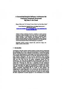
Fig. 3. Modal analysis of a lithographic system in support of the design of an active vibration controller needed for enabling image precision to a few nanometers. Shown is the 76th vibration mode, an internal component response. FE model size: 602,070 dofs. Machine: ASCI Red. Processors used: 50 processors.

ware, Salinas is an implicit code and therefore primarily requires a scalable equation solver in order to meet its objectives. Because all ASCI machines are massively parallel computers, the definition of scalability adopted here is the ability to solve an  -times larger problem using an  -times larger number of processors 

in a nearly constant CPU time. Achieving this definition of scalability requires an equation solver which is (a) numerically scalable — that is, whose arithmetic complexity grows almost linearly with the problem size, and (b) amenable to a scalable parallel implementation — that is, which can exploit as large an  as possible while incurring relatively small interprocessor communication costs. Such a stringent definition of scalability rules out sparse direct solvers because their arithmetic complexity is a nonlinear function of the problem size. On the other hand, several multilevel [2] iterative schemes such as multigrid algorithms [3, 4, 5] and domain decomposition (DD) methods with coarse auxiliary problems [6, 7, 8] can be characterized by a nearly linear arithmetic complexity, or an iteration count which grows only weakly with the size of the problem to be solved. Salinas selected the DD-based FETI-DP iterative solver [9, 10] because of its underlying structural mechanics concepts, its robustness and versatility, its provable numerical scalability [11, 12], and its established scalable performance on massively parallel processors. Our submission focuses on an engineering software with more than 100,000 lines of code and a long list of users. Salinas contains several computational modules including those for forming and assembling the element stiffness, mass, and damping matrices, recovering the strain and stress fields, performing sensitivity analysis, 3

solving generalized eigenvalue problems, and time-integrating by implicit schemes semi-discrete equations of motion. Furthermore, our submission addresses total solution time, scalability, and overall CPU efficiency in addition to floating-point performance. Salinas was developed with code portability in mind. By 1999, it had demonstrated scalability [13] on 1,000 processors of ASCI Red [36]. Currently, it runs routinely on ASCI Red and ASCI White [37], performs equally well on the CPLANT New Mexico [38] cluster of 1,500 Compaq XP1000 processors, and is supported on a variety of sequential and parallel workstations. On 2,940 processors of ASCI Red, Salinas sustains 292.5 Gflop/s — that is, 99.5 Mflop/s per ASCI Red processor, and an overall CPU efficiency of 30%. On 3,375 processors of ASCI White, Salinas sustains 1.16 Tflop/s — that is, 343.7 Mflop/s per processor, and an overall CPU efficiency of 23%. These performance numbers are well above what is commonly considered achievable by unstructured FE-based software. To the best of our knowledge, Salinas is today the only FE software capable of computing a dozen eigen modes for a million-dof FE structural model in less than 10 minutes. Given the pressing need for such computations, it is rapidly becoming the model for parallel FE analysis software in both academic and industrial structural mechanics/dynamics communities [14].

2 The Salinas software



and uses 64-bit arithmetic. It combines a modern Salinas is mostly written in object-oriented FE software architecture, scalable computational algorithms, and existing high-performance numerical libraries. Extensive use of high-performance numerical building block algorithms such as the Basic Linear Algebra Subprograms (BLAS), the Linear Algebra Package (LAPACK), and the Message Passing Interface (MPI) has resulted in a software application which features not only scalability on thousands of processors, but also a solid per-processor performance and the desired portability.

2.1 Distributed architecture and data structures

The architecture and data structures of Salinas are based on the concept of DD. They rely on the availability of mesh partitioning software such as CHACO [15], TOP/DOMDEC [16], METIS [17], and JOSTLE [18]. The distributed data structures of Salinas are organized in two levels. The first-level supports all local computations as well as all interprocessor communication between neighboring subdomains. The second level interfaces with those data structures of an iterative solver 4

which support the global operations associated with the solution of coarse problems. 2.2 Analysis capabilities

Salinas includes a full library of structural finite elements. It supports linear multiple point constraints (LMPCs) to provide modeling flexibility, geometrical nonlinearities to address large displacements and rotations, and limited structural nonlinearities to incorporate the effect of joints. It offers five different analysis capabilities: (a) static, (b) modal vibration, (c) implicit transient dynamics, (d) frequency response, and (e) sensitivity. The modal vibration capability is built around ARPACK’s Arnoldi solver [19], and the transient dynamics capability is based on the implicit “generalized ” time-integrator [20]. All analysis capabilities interface with the same FETI-DP module for solving the systems of equations they generate.

3 The FETI-DP solver

3.1 Background Structural mechanics problems can be subdivided into second-order and fourthorder problems. Second-order problems are typically modeled by bar, plane stress/strain, and solid elements, and fourth-order problems by beam, plate, and shell elements. The condition number of a generalized symmetric stiffness matrix  arising from the FE discretization of second-order problems grows asymptotically with the mesh size  as

  

(1)

and that of a generalized symmetric stiffness matrix arising from the FE discretization of a fourth-order problem grows asymptotically with  as

  

(2)

The above conditioning estimates explain why it was not until powerful and robust preconditioners became recently available that the method of Conjugate Gradients (CG) of Hestenes and Steifel [21] made its debut in production commercial FE structural mechanics software. Material and discretization heterogeneities as well as bad element aspect ratios, all of which are common in real-world FE models, worsen further the above condition numbers. 5

H

h

Fig. 4. Mesh size

and subdomain size ! .

3.2 A scalable iterative solver

FETI (Finite Element Tearing and Interconnection) is the generic name for a suite of DD based iterative solvers with Lagrange multipliers designed with the condition number estimates (1) and (2) in mind. The first and simplest FETI algorithm, known as the one-level FETI method, was developed around 1989 [23, 24]. It can be described as a two-step Preconditioned Conjugate Gradient (PCG) algorithm where subdomain problems with Dirichlet boundary conditions are solved in the preconditioning step, and related subdomain problems with Neumann boundary conditions are solved in a second step. The one-level FETI method incorporates a relatively small-size auxiliary problem which is based on the rigid body modes of the floating subdomains. This coarse problem accelerates convergence by propagating the error globally during the PCG iterations. For second-order elasticity problems, the condition number of the interface problem associated with the one-level FETI method equipped with the Dirichlet preconditioner [25] grows at most polylogarithmically with the number of elements per subdomain

"

, +  $#&%('*)  

(3)

Here, + denotes the subdomain size (Fig. 4) and therefore +-  is the number of elements along each side of a uniform subdomain. The condition number estimate (3) constitutes a major improvement over the conditioning result (1). More importantly, it establishes the numerical scalability of the FETI method with respect to the problem size, the number of subdomains, and the number of elements per subdomain. For fourth-order plate and shell problems, preserving the quasi-optimal condition number estimate (3) requires enriching the coarse problem of the one-level FETI method by the subdomain corner modes [27, 28]. This enrichment transforms the original one-level FETI method into a genuine two-level algorithm known as the two-level FETI method [27, 28]. Both the one-level and two-level FETI methods have been extended to transient dynamics problems as described in [26]. 6

Unfortunately, enriching the coarse problem of the one-level FETI method by the subdomain corner modes increases its computational complexity to a point where the overall scalability of FETI is diminished on a very large number of processors, 21*1*1 . For this reason, the basic principles governing the design of say . 0/  the two-level FETI method were recently revisited to construct a more efficient dual-primal FETI method [9, 10] known as the FETI-DP method. This most recent FETI method features the same quasi-optimal condition number estimate (3) for both second- and fourth-order problems, but employs a more economical coarse problem than the two-level FETI method. Mainly for this reason, FETI-DP was chosen to power Salinas.

3.3 A versatile iterative solver

Production codes such as Salinas require their solver to be sufficiently versatile to address, among others, problems with successive right-hand sides and/or LMPCs. Systems with successive right-hand sides arise in many structural applications including static analysis for multiple loads, sensitivity, modal vibration, and implicit transient dynamics analyses. Krylov-based iterative solvers are ill-suited for these problems, unless they incorporate special techniques for avoiding restarting the iterations from scratch for each different right-hand side [29, 30, 31, 32]. To address this issue, Salinas’ FETI-DP solver is equipped with the projection/reorthogonalization procedure described in [30, 31]. This procedure accelerates convergence as illustrated below. Fig. 5 reports the performance results obtained for FETI-DP equipped with the projection/re-orthogonalization technique proposed in [30, 31] and applied to the solution of the repeated systems arising from the computation of the first 50 eigen modes of the optical shutter shown in Fig. 5(a). These results are for a FE structural model with 16 million dofs, and a simulation performed on 1,071 processors of ASCI White. As shown in Fig. 5(b), the number of FETI-DP iterations is equal to 75 for the first right-hand side, and drops to 26 for the 100th. Consequently, the CPU time for FETI-DP drops from 57.0 seconds for the first problem — 33.4 seconds of which correspond to a one-time preprocessing computation — to 10.7 seconds for the last one. The total FETI-DP CPU time for all 100 successive problems is equal to 1,223 seconds. Without the projection/re-orthogonalization-based acceleration procedure, the total CPU consumption by FETI-DP for all 100 successive problems is equal to 2,445 seconds. Hence, for this modal analysis, our acceleration scheme reduces the CPU time of FETI-DP by a factor equal to 2, independently of the parallelism of the computation. LMPCs are frequent in structural analysis because they ease the FE modeling of complex structures. They can be written in matrix form as 34 65 , where 3 is 7

(a) Left: optical shutter to be embedded in a MEMS device. Right: von Mises stresses associated with an eigen mode.

(b) Iteration count and CPU time for each successive linear solve. Fig. 5. Modal analysis of an optical shutter embedded in a MEMS device. Performance results of FETI-DP for the solution of the 100 linear solves arising during the computation of the first 50 eigen modes. FE model size: 16,000,000 dofs. Machine: ASCI White. Processors used: 1,071 processors.

a rectangular matrix, 5 is a vector, and 4 is the solution vector of generalized displacements. Solving systems of equations with LMPCs by a DD method is not an easy task because LMPCs can arbitrarily couple two or more subdomains. To address this important issue, a methodology was presented in [33] for generalizing numerically scalable DD-based iterative solvers to the solution of constrained FE systems of equations, without interfering with their local and global precondi8

tioners. FETI-DP incorporates the key elements of this methodology, and therefore naturally handles LMPCs.

4 Optimization of solution time and scalability

The performance and scalability of Salinas are essentially those of its FETI-DP module applied to the solution of a problem of the form

 4 7

(4)

where  arises from any of Salinas’ analysis capabilities. Given a mesh partition, FETI-DP transforms the above global problem into an interface problem with Lagrange multiplier unknowns, and solves this problem by a PCG algorithm. The purpose of the Lagrange multipliers is to enforce the continuity of the generalized displacement field 4 on the interior of the subdomain interfaces. Each iteration of the PCG algorithm incurs the solution of a set of sparse subdomain problems with Neumann boundary conditions, a related set of sparse subdomain problems with Dirichlet boundary conditions, and a sparse coarse problem of the form

 9:;8 :=< : > :

(5)

In Salinas, the independent subdomain problems are solved concurrently by the sequential block sparse Cholesky algorithm described in [34]. This solver uses BLAS level 3 operations for factoring a matrix, and BLAS level 2 operations for performing forward and backward substitutions. For solving the coarse problem (5), two approaches are available. In the first approach [13], the relatively small sparse matrix  :;8 : is duplicated in each processor which factors it. In a preprocessing step, the inverse of this matrix,  :;8@: ?BAC , is computed by embarrassingly parallel forward and backward substitutions and stored

ML*NPO across all  processors in the column-wise distributed format DFEB :;8G:I ?BAC H KJ ML  . Given that the solution of the coarse problem (5) can be written as

ML*NPO

< :   :;8 : ?BAC > : 

EQ :;8 :I ?RASC H TE > : H

 , L



(6)

it is computed in parallel using local matrix-vector products and a single global range communication. In the second approach,  :;8 : is stored in a scattered column

data structure across an optimal number of processors  U V . , and the coarse problem (5) is solved by a parallel sparse direct method which resorts to selective 9

inversions for improving the parallel performance of forward and backward substitutions [39]. When  :;8 : can be stored in each processor, the first approach maximizes the floatingpoint performance. For example, when Salinas’ FETI-DP uses the first approach for solving the coarse problems, it sustains 150 Mflop/s per ASCI Red processor rather than the 99.5 Mflop/s announced in the introduction. However, when the size of  :W8 : is greater or equal to the average size of a local subdomain problem, the second approach scales better than the first one and minimizes the CPU time. For these reasons, Salinas selects the first method when the size of the coarse problem is smaller than the average size of a local subdomain problem, and the second method otherwise.

5 Performance and scalability studies

5.1 Focus problems

To illustrate the scalability properties, parallel performance, and CPU efficiency of Salinas and FETI-DP, we consider the static analysis of two different structures. We remind the reader that because Salinas is an implicit code, its performance for static analysis is indicative of its performance for its other analysis capabilities. The first structure, a cube, defines a model problem which has the virtue of simplifying the tedious tasks of mesh generation and partitioning during scalability studies. We partition this cube into YXZ\[]_Z` ^ []_Za subdomains, and discretize each subdomain by _b[cYbd[cYb 8-noded hexahedral elements. The second structure is the optical shutter introduced in Section 3.3. This realworld structure is far more complex than suggested by Fig. 5(a), as its intricate microscopic geometrical features are hard to visualize. It is composed of three disk layers that are separated by gaps, but connected by a set of flexible beams extending in the direction normal to all three disks (see Fig. 7). We construct two detailed (see Fig. 8) FE models of this real-world structure: model M1 with 16 million dofs, and model M2 with 110 million dofs. We use CHACO [15] to decompose the FE model M1 into 288, 535, 835, and 1,071 subdomains, and the FE model M2 into 3,783 subdomains. We recognize that for the cube problem, load balance is ensured by the uniformity of each mesh partition, and note that for the optical shutter problem, load balance depends on the generated mesh partition. In all cases, we map one processor onto one subdomain. 10

Fig. 6. The cube problem: e = 30.0e+6 fhgji , kmlonKprq — s s b t s b t s b subdomain discretization.

XZut s ^Z t s aZ partition and uniform

Fig. 7. Optical shutter with a 500 micron diameter and a three-layer construction.

5.2 Measuring performance

All CPU timings reported in the remainder of this paper are wall clock timings obtained using the C/C++ functions available in v time.h / . On ASCI Red, we use the performance library of this machine, perfmon, to measure the floating-point performance of Salinas. The floating-point performance shown on ASCI RED in the subsequent figures is for the solver (FETI-DP) stage of Salinas only. However, the Salinas execution times measured on ASCI Red include all the stages from beginning the end except the input/output stage. On ASCI White, we use the hpmcount utility[35] provided by IBM to measure floating-point performance of Salinas. None of Salinas was excluded from the floating-point measurement on ASCI White. The Salinas execution times on ASCI White include the input/output stage. 11

Fig. 8. Meshing complexity of the optical shutter.

We measure the overall CPU efficiency as follows CPU Efficiency xw`y{z,|T}

7

5 };y~F-*€ 4 €‚  . ~*ƒhy…„,†K€‡€ˆyƒh€  . ‰[‹Š K† |TŒ‡Ž

(7)

where Š †K|TŒ‡Ž is the peak processor floating-point rate and is equal to 333 Mflop/s for an ASCI Red processor, and 1,500 Mflop/s for an ASCI White processor.

5.3 Scalability and overall CPU efficiency on ASCI Red For the cube problem, we fix _b  M and vary  XZ ,  ^Z and  aZ to increase the size of the global problem from less than a million to more than 36 million dofs. We note that the parameters of this problem are such that in all cases, Salinas chooses the parallel sparse direct method described in [39] for solving the coarse problems. 12

Fig. 9. Static analysis of the cube on ASCI Red: scalability of FETI-DP and Salinas for a fixed-size subdomain and an increasing number of subdomains and processors.

Fig. 10. Static analysis of the cube on ASCI Red: overall CPU efficiency and aggregate floating-point rate achieved by Salinas.

Fig. 9 highlights the scalability of FETI-DP and Salinas on ASCI Red. More specifically, it shows that when the number of subdomains, and therefore the problem size, as well as . are increased, the number of FETI-DP iterations remains relatively constant and the total CPU time consumed by FETI-DP increases only slightly. Fig. 10 shows that the floating-point rate achieved by Salinas increases linearly with  and reaches 292.5 Gflop/s on 2,940 processors. This corresponds to a performance of 99.5 Mflop/s per processor. Consequently, Salinas delivers an overall CPU efficiency ranging between 34% on 64 processors and 30% on 2,940 processors.

13

Fig. 11. Static analysis of the cube on ASCI White: scalability of FETI-DP for a fixed-size subdomain and an increasing number of subdomains and processors.

5.4 Scalability and overall CPU efficiency on ASCI White

5.4.1 The cube problem Here, we fix Y‘“’•”*” because each ASCI White processor has a larger memory than an ASCI Red processor, and vary Y–— , Y˜— and Y™— to increase the size of the global problem from 2 million to more than 100 million dofs. For _‘c’š”*” , the size of the coarse problem is smaller than the size of the subdomain problem and therefore Salinas chooses the first method described in Section 4 for solving the coarse problems. Fig. 11 highlights the scalability of FETI-DP and Salinas on ASCI White. It shows that when ›œ is increased with the size of the global problem, the iteration count and CPU time of FETI-DP remain relatively constant. Furthermore, Fig. 12 shows that the floating-point rate achieved by Salinas on ASCI White increases linearly with ›œ and reaches 1.16 Tflop/s on 3,375 processors. This corresponds to an average performance of 343.7 Mflop/s per processor. Consequently, Salinas delivers an overall CPU efficiency ranging between 28% on 64 processors and 24% on 3,375 processors.

5.4.2 The real-world optical shutter problem To illustrate the parallel scalability of Salinas for a fixed-size global problem, we report in Fig. 13 the speed-up obtained when using the FE model M1 and increasing the number of ASCI White processors from 288 to 1,071. The reader can observe a linear speed-up for this range of processors which is commensurate with the size of the FE model M1. 14

Fig. 12. Static analysis of the cube on ASCI White: overall CPU efficiency and aggregate floating-point rate achieved by Salinas.

Fig. 13. Static analysis of the optical shutter on ASCI White: speed-up of Salinas for the FE model M1 with 16,000,000 dofs.

Next, we summarize in Table 1 the performance results obtained on ASCI White for the larger FE model M2. The floating-point rate and overall CPU efficiency achieved in this case are lower than those obtained for the cube problem because the nontrivial mesh partitions generated for the optical shutter are not well balanced. Balancing a mesh partition for a DD method in which the subdomain problems are solved by a sparse direct method requires balancing the sparsity patterns of the subdomain problems, which is difficult to achieve without increasing the cost of the partitioning process itself. Still, we point out the remarkable fact that Salinas performs the static analysis of a complex 110 million dofs FE model on 3,375 ASCI White processors in less than 7 minutes and sustains 745 Gflop/s during this process. 15

FE

Size



model M2

110,000,000 dofs

3,783

Solution

Performance

Overall CPU

Time

Rate

Efficiency

418 seconds

745 Gflop/s

13%

Table 1 Static analysis of the optical shutter on 3,783 ASCI White processors: performance of Salinas for the FE model M2.

6 Conclusions

This submission focuses on Salinas, an engineering software with more than 100,000  lines of code and a long list of users. In the context of unstructured applications, the 292.5 Gflop/s sustained by this software on 2,940 ASCI Red nodes using 1 CPU/node (2,940 processors) compares favorably with the most recent and impressive performances: 156 Gflop/s on 2,048 nodes of ASCI Red using 1 CPU/node (2,048 processors) demonstrated by a winning entry in 1999 [40], and 319 Gflop/s on 2,048 nodes of ASCI Red using 2 CPUs/node (4,096 processors) demonstrated by another winning entry also in 1999 [41]. Yet, the highlight of this submission is the sustained performance of 1.16 Tflop/s on 3,375 processors of ASCI White by a code capable of various structural analyses of real-world FE models with more than 100 million dofs, is supported on a wide variety of platforms, and is inspiring the development of parallel FE software throughout both academic and industrial structural mechanics communities.

Acknowledgments

Salinas code development has been ongoing for several years and would not have been possible if not for the help from the following people: Dan Segalman, John Red-Horse, Clay Fulcher, James Freymiller, Todd Simmermacher, Greg Tipton, Brian Driessen, Carlos Felippa, David Martinez, Michael McGlaun, Thomas Bickel, Padma Raghavan, and Esmond Ng. The authors would also like to thanks the support staff of ASCI Red and ASCI White for their indispensable help. Sandia is a multiprogram laboratory operated by Sandia Corporation, a Lockheed Martin Company, for the U.S. Department of Energy (DOE) under Contract No. DEAC04-94AL85000. Charbel Farhat acknowledges partial support by Sandia under Contract No. BD-2435, and partial support by DOE under Award No. B347880/W740-ENG-48. Michel Lesoinne acknowledges partial support by DOE under Award No. B347880/W-740-ENG-48. 16

References [1] M. S. Eldred, A. A. Giunta, B. G. van Bloemen Waanders, S. F. Wojtkiewicz, W. E. Hart and M. P. Alleva. DAKOTA, a multilevel parallel object-oriented framework for design optimization, parameter estimation, uncertainty quantification, and sensitivity analysis. Version 3.0 reference manual. Sandia Technical Report SAND2001-3515, 2002. [2] S. F. McCormick. Multilevel adaptive methods for partial differential equations. Frontiers in Applied Mathematics, SIAM, 1989. [3] S. F. McCormick, ed. Multigrid methods. Frontiers in Applied Mathematics, SIAM, 1987. [4] W. Briggs. A multigrid tutorial. SIAM, 1987. [5] P. Vanek, J. Mandel and M. Brezina. Algebraic multigrid on unstructured meshes. Computing 56, 179-196 (1996). [6] P. LeTallec. Domain-decomposition methods in computational mechanics. Computational Mechanics Advances 1, 121-220 (1994). [7] C. Farhat and F. X. Roux. Implicit parallel processing in structural mechanics. Computational Mechanics Advances 2, 1-124 (1994). [8] B. Smith, P. Bjorstad and W. Gropp. Domain decomposition, parallel multilevel methods for elliptic partial differential equations. Cambridge University Press, 1996. [9] C. Farhat, M. Lesoinne and K. Pierson. A scalable dual-primal domain decomposition method. Numer. Lin. Alg. Appl. 7, 687-714 (2000). [10] C. Farhat, M. Lesoinne, P. LeTallec, K. Pierson and D. Rixen. FETI-DP: a dual-primal unified FETI method - part I: a faster alternative to the two-level FETI method. Internat. J. Numer. Meths. Engrg. 50, 1523-1544 (2001). [11] J. Mandel and R. Tezaur. On the convergence of a dual-primal substructuring method. Numer. Math. 88, 543-558 (2001). [12] A. Klawonn and O. B. Widlund. FETI-DP methods for three-dimensional elliptic problems with heterogeneous coefficients. Technical report, Courant Institute of Mathematical Sciences, 2000. [13] M. Bhardwaj, D. Day, C. Farhat, M. Lesoinne, K. Pierson and D. Rixen. Application of the FETI method to ASCI problems: scalability results on onethousand processors and discussion of highly heterogeneous problems. Internat. J. Numer. Methds. Engrg. 47, 513-536 (2000). [14] J. J. McGowan, G. E. Warren and R. A. Shaw. Whole ship models. The ONR Program Review, Arlington, April 15-18, 2002. [15] B. Hendrickson and R. Leland. The Chaco User’s Guide: Version 2.0. Sandia Tech. Report SAND94-2692, 1994. [16] C. Farhat, S. Lant´eri and H. D. Simon. TOP/DOMDEC, a software tool for mesh partitioning and parallel processing. Comput. Sys. Engrg. 6, 13-26 (1995). [17] G. Karypis and V. Kumar. Parallel multilevel k-way partition scheme for irregular graphs. SIAM Review 41, 278-300 (1999). [18] C. Walshaw and M. Cross. Parallel optimization algorithms for multilevel mesh partitioning. Parallel Comput. 26, 1635-1660 (2000). 17

[19] R. Lehoucq, D. C. Sorensen, C. Yang. Arpack User’s Guide: Solution of largescale eigenvalue problems with implicitly restarted Arnoldi methods. SIAM, 1998. [20] J. Chung and G. M. Hulbert. A time integration algorithm for structural dynamics with improved numerical dissipation: the generalized- method. J. Appl. Mech. 60, 371 (1993). [21] M. R. Hestenes and E. Steifel. Method of conjugate gradients for solving linear systems. J. Res. Nat. Bur. Standards 49, 409-436 (1952). [22] G. H. Golub and C. F. Van Loan. Matrix computations. The Johns Hopkins University Press, 1990. [23] C. Farhat. A Lagrange multiplier based divide and conquer finite element algorithm. J. Comput. Sys. Engrg. 2, 149-156 (1991). [24] C. Farhat and F. X. Roux. A method of finite element tearing and interconnecting and its parallel solution algorithm. Internat. J. Numer. Meths. Engrg. 32, 1205-1227 (1991). [25] C. Farhat., J. Mandel and F. X. Roux. Optimal convergence properties of the FETI domain decomposition method. Comput. Meths. Appl. Mech. Engrg. 115, 367-388 (1994). [26] C. Farhat, P. S. Chen and J. Mandel. A scalable Lagrange multiplier based domain decomposition method for implicit time-dependent problems. Internat. J. Numer. Meths. Engrg. 38, 3831-3858 (1995). [27] C. Farhat and J. Mandel. The two-level FETI method for static and dynamic plate problems - Part I: an optimal iterative solver for biharmonic systems. Comput. Meths. Appl. Mech. Engrg. 155, 129-152 (1998). [28] C. Farhat, P. S. Chen, J. Mandel and F. X. Roux. The two-level FETI method - Part II: extension to shell problems, parallel implementation and performance results. Comput. Meths. Appl. Mech. Engrg. 155, 153-180 (1998). [29] Y. Saad. On the Lanczos method for solving symmetric linear systems with several right-hand sides. Math. Comp. 48, 651-662 (1987). [30] C. Farhat and P. S. Chen. Tailoring Domain Decomposition Methods for Efficient Parallel Coarse Grid Solution and for Systems with Many Right Hand Sides. Contemporary Mathematics 180, 401-406 (1994). [31] C. Farhat, L. Crivelli and F. X. Roux. Extending substructure based iterative solvers to multiple load and repeated analyses. Comput. Meths. Appl. Mech. Engrg. 117, 195-209 (1994). [32] P. Fischer. Projection techniques for iterative solution of Ax=b with successive right-hand sides. Comp. Meths. Appl. Mech. Engrg. 163, 193-204 (1998). [33] C. Farhat, C. Lacour and D. Rixen. Incorporation of linear multipoint constraints in substructure based iterative solvers - Part I: a numerically scalable algorithm. Internat. J. Numer. Meths. Engrg. 43, 997-1016 (1998). [34] E. G. Ng and B. W. Peyton. Block sparse cholesky algorithms. SIAM J. Sci. Stat. Comput. 14, 1034-1056 (1993). [35] Information on hpmcount, a performance monitor utility that reads hardware counters for IBM SP RS/6000 computers. http://www.alphaworks.ibm.com/tech/hpmtoolkit. 18

[36] ASCI Red Home Page. http://www.sandia.gov/ASCI/Red. [37] ASCI White Home Page. http://www.llnl.gov/asci/platforms/white. [38] ASCI CPLANT Home Page. http://www.cs.sandia.gov/cplant. [39] P. Raghavan. Efficient parallel triangular solution with selective inversion. Parallel Processing Letters 8, 29-40 (1998). [40] K. Anderson, W. Gropp, D. Kaushik, D. Keyes and B. Smith. Achieving high sustained performance in an unstructured mesh CFD application. Proceedings of SC99, Portland, OR, November 1999. [41] H. M. Tufo and P. F. Fischer. Terascale spectral element algorithms and implementations. Proceedings of SC99, Portland, OR, November 1999.

19