SALSA: A Language for Search Algorithms

Submitted to the CP’98 special issue of CONSTRAINTS

SALSA : A Language for Search Algorithms François Laburthe, Yves Caseau Bouygues – e-lab 1 av. E. Freyssinet 78061 St Quentin en Yvelines, FRANCE {flaburthe;ycs}@bouygues.com

Abstract: Constraint Programming is recognized as an efficient technique for solving hard combinatorial optimization problems. However, it is best used in conjunction with other optimization paradigms such as local search, yielding hybrid algorithms with constraints. Such combinations lack a language supporting an elegant description and retaining the original declarativity of Constraint Logic Programming. We propose a language, SALSA, dedicated to specifying (local, global or hybrid) search algorithms. We illustrate its use on a few examples from combinatorial optimization for which we specify complex optimization procedures with a few simple lines of code of high abstraction level. We report preliminary experiments showing that such a language can be implemented on top of CP systems, yielding a powerful environment for combinatorial optimization.

1. Introduction Today, combinatorial problem solving is one of the most successful fields of application for Constraint Programming (CP). In the past few years, on problems such as scheduling, resource allocation, crew rostering, fleet dispatching, etc., the CP technology has risen to a state-of-the-art level on academic problems as well as on some real-life industrial ones (see the PACT, Ilog Users or CHIP Users conferences). However, in many cases where the constraint approach has proven really successful, the standard resolution procedure was not used and a more customized search was applied. In some sense, many CP approaches have left the framework of Constraint Logic Programming (CLP) [JL 87], and belong to the more general case of hybrid optimization algorithms. Indeed, the default search procedure offered by today's CP systems is inherited from logic programming systems (Prolog's SLD resolution strategy [Llo 87]). Since constraint propagation is incomplete for most finite domain constraints used in combinatorial problem solving (e.g. this is the case for almost all “global” constraints [Be 00]), a search tree is explored, where each node corresponds to the labeling of one of the variables involved in the goal by one of the values in its domain). Upon failure in one of the branches, the algorithm backtracks to the previous node and tries to assign to the variable the next value from its domain. This search tree is visited by a depth-first exploration, in order to limit memory requirements. In the case of optimization problems, two strategies are available, either a new search is started each time a solution is found (constraining the objective function to take a better value), or the objective is dynamically constrained to be better than the best solution found so far (branch&bound search). Many Constraint Programming applications have considered other search strategies for the following reasons :

1


• Such a global search may not be the best method for obtaining a first solution (tailored greedy heuristics performing a limited amount of look-ahead search may be more efficient, for example in scheduling [DT 93] or routing [CL 99b]). • It may be a good idea to incorporate a limited amount of breadth-first search (such as the “shaving” mechanism used for scheduling [MS 96]), • Other visiting orders of the search tree may sometimes be worthwhile (e.g. LDS [HG 95], [CL 99b], A*), • It may be interesting to express topological conditions on the shape of the sub-tree that is explored (unbalanced trees, limited number of nodes, limited number of choices along a branch, ...) This is actually an old idea of logic programming to separate logic and control and to specify both with a separate language [Ko 79]. Several extensions of logic programming have been proposed in order to control search [Na 84], [He 87] [HS98].From the early CLP languages to the more recent modeling languages, such as OPL Studio [VH99], optimization tools have always supported elegant descriptions of a problem’s logic. But only recently have CP tools focused on control: Like Oz explorer [Sch 97], Ilog Parallel Solver [Pe 99] and Visual CHIP [SA 99], SALSA provides the user with the ability to specify the way the global search tree is visited. Moreover, combinatorial problem solving with constraints is also expanding beyond the scope of global search by considering hybrid combinations of constraint propagation and global search with other paradigms, such as local optimization and greedy heuristics. This shift can be easily understood for two reasons : • Global search may be applied successfully only if the algorithm is given enough time to visit a significant portion of the solution space. For large problems, such a thorough exploration is out of reach, hence other approaches should be considered. • In the past decades, Operations Researchers have proposed a variety of algorithms dedicated to specific optimization problems, many of which are extremely efficient. This wealth of knowledge should be used as much as possible within CP. The recent trend of large and variable neighborhoods [MH 97] [Sh 98] [BV 98] in local optimization is particularly interesting. This interest in composing algorithms is thus not limited to global search methods but also concerns the assembly of simple local search methods into more complex ones. There are many ways in which CP may be combined with local optimization : -

global search can be used to find a first solution by global search before turning to local search for further improvements

-

local search can be applied at each node of a global search tree, in order to optimize the current partial solution [CL 99a]

-

global search can be used to find a good move within a neighborhood [LK 73]. For instance, the neighborhood can be defined through domain variables and branch & bound may be used to search for the best neighbor. Another possibility

2


consists in keeping only a fragment of the solution and trying a limited global search to extend it [CL 99a]. In practice, programming such algorithms is a tedious and error-prone task, for lack of a high-level language : CP tools do not offer the ability to perform non-monotonic operations (which are the basis of local search algorithms) and other tools dedicated to one specific optimization paradigm (MIP [FMK 93] or local optimization [MVH 97]) do not offer the possibility to post constraints or to perform hypothetical reasoning. Thus, the programmer of hybrid algorithms is left with an imperative language which most of the time lacks abstraction and declarativity (such as C++). In order to offer an environment for programming such hybrid algorithms, we propose to consider logic and control separately and to use a specific language, SALSA, in order to control the search for solutions. SALSA is not a standalone language but works in cooperation with a host programming language. We will demonstrate how SALSA can be used to program local, global and hybrid search procedures. The paper is organized as follows. Section 2 discusses the basis of search algorithms, neighborhoods and choices, and informally introduces the main ideas of SALSA. Section 3 introduces SALSA on a simple example, while section 4 describes SALSA’s grammar. Section 5 presents an operational semantics while section 7 goes through a set of illustrative examples.

2. Transitions, choices and neighborhoods Local and global search algorithms have many features in common. First, they search for solutions (configurations of a system) within some search space. Thus, an execution of a search algorithm may be represented by a sequence of states, tracing the sequence of points which have been visited in the search space. For local search, states are (feasible) solutions: they can be interpreted as (valid) answers to the optimization problem. On the contrary, for global search, states may be partial solutions: this is the case with constructive methods, such as CP, when only a fraction of the variables have been instantiated. A search algorithm can thus be described by the mechanism responsible for driving the execution from one state to the next one. Such moves from one configuration to another are chosen among several possible ones : local search only considers one move among the set, whereas global search comes back to the choice point until all possible branches (moves) have been considered. If we describe such a system by a non-deterministic automaton, each visited state can be traced back from the start state by a sequence of transitions. In addition, global search also considers backward moves (going back in time to a previously visited state). SALSA allows the programmer to specify those choice mechanisms that are responsible for generating moves in an elegant manner and it offers primitives for composing such transitions.

2.1 Global search Search trees are always built by decomposing a problem into sub-problems. For CP, separation is achieved by instantiating one of the variables or posting an additional

3


constraint and propagating. For MIP (Mixed Integer Programming), separation is achieved by instantiating a variable, refining the bound of some variable, or posting additional cuts. Global search algorithms are usually specified by the order in which variables should be instantiated; this order may be static or dynamic. Such descriptions can also be refined by hierarchical decompositions : the overall problem is then described as a set of sub-problems, with associated sub-goals and subsets of variables to instantiate. Another standpoint consists of describing the search algorithms in a framework of distributed computation : the state corresponds to the computation environment (the constraint store), and branching corresponds to process cloning. A process is associated with each node; copies of the current process are made at a choice point (one copy per branch), and the corresponding transitions are evaluated in the computation environment of the new process. Such formalisms providing an explicit access to the state, enable the user to program any exploration strategy, such as A* [Pea 84]. For instance, in Oz [SS 94], processes are named and can be stored in variables or passed as arguments to functions. With Ilog Parallel Solver [Pe 99], the programmer has no direct access to the node, the search algorithm is specified with goals. Arbitrary functions may be defined on goals in order to change the order of evaluation of nodes or to select the subset of nodes in the search tree that will be visited. 2.2 Local search The LOCALIZER language has been proposed for local search algorithms [MVH 97]. Such algorithms programmed in this elegant framework feature three components : 1. Invariants : these invariants are used to introduce functional dependencies between data structures. In addition to the basic data structures used to represent a solution, some additional data structures are used to store redundant information. Their values are specified by means of a formula called an invariant. Such formulae, which are in a sense similar to constraints, are used to maintain consistent values in the additional data structures each time a value of the basic data is modified. Unlike constraints, invariants specify in a declarative manner the non-monotonic evolution of data. There is no such notion like domain shrinking, all variables are always instantiated. 2. Neighborhoods : they correspond to the moves that can be applied to go from one state to another. They are described by imperative updates on basic data which trigger some computations, in order to maintain the invariants. 3. Control : the control flow of the algorithm is described in two places. The global search procedure is always made of two nested loops (at most MaxTries random walks, each of which is composed of at most MaxIter moves). In addition, one may add local conditions that will be used for selecting the move in the neighborhood : moves may be sorted or selected according to a given probability, etc. Hence, with such a description, a local search algorithm can be easily adapted from hill-climbing to tabu search or from a random walk to simulated annealing, by adding a few conditions specifying when to accept a move or not.

4


2.3 Hybrid search The formalisms for global and local search differ : in global search, goals and constraints describe properties of final states, while in local search, invariants and neighborhoods describe properties of all states. However, if we further decompose global search algorithms, the basic branching mechanism is very much like that of local search : from a state, we consider several decisions (instantiating a variable to one of the values in its domain, or enforcing one among a set of constraints), each leading to a different state, and we only choose one of them at a time. Thus, a language expressing neighborhoods (in local search) and choices (in global search) in the same formalism would be able to express hybrid combinations. This is what SALSA does : • Choices are specified in a manner similar to LOCALIZER's neighborhoods. Transitions correspond to the evaluation of an expression, and some local control can be specified at the choice level (specifying which transitions are valid ones, in what order they should be considered, recognizing local optima, etc. ). • Such choices are reified as objects, which can in turn, be composed by a set of operators, in order to specify search algorithms. The result is a language for search algorithms, which can elegantly describe local search procedures, global search algorithms, and many combinations. 2.4 Encapsulating consistency mechanism in solvers Local and global search both use consistency mechanisms. The programmer of a local search algorithm maintains some data structures through invariants without explicitly specifying the effect of moves on such data. In the same spirit, in global search, the programmer only states a constraint to be added to the problem and she relies on a black-box engine for computing all consequences of this addition. In both cases, some computations are triggered, be it production rules, propagation daemons or pivoting operations in a simplex tableau. In the remainder of the article, we assume that the programmer is able to define some objects called solvers, that encapsulate such behaviors for maintaining consistency. We do not describe how such solvers may be programmed and composed, which is a line of research of its own, out of the scope of this article. The only interface that we use will be to post events to solvers: each time we use the syntax post(S,e), S will be responsible for triggering some consistency computations after the evaluation of the expression e. The execution of such event posts can have two effects : •

it always modifies some data structures,

•

it may detect a failure when the problem associated to the current node is infeasible.

In the examples of section 5, we use several such solvers: FD for finite domain propagation, SAT for Boolean satisfaction algorithms, schedule for scheduling constraint propagation, dispatch for routing constraint propagation and LK for the Lin and Kernighan TSP heuristic. The paper does not address the issue of combining different solvers over the same data structures: for instance, applying both an invariant

5


and a propagation solver on the same variables would require the definition of event handling strategies in order to avoid inconsistent solver states. All our examples use one solver per domain, in order to avoid solver cooperation issues. From a system point of view, the current implementation of SALSA currently only supports solvers that are available as CLAIRE source libraries (there is therefore no separate compilation). From a software architecture point of view, the separation of solvers from the tree search control requires that the controller (SALSA’s main function) broadcasts orders to the solvers for navigating through the search tree (going up and down the branches).

3. A simple example This section introduces the SALSA language on a simple example: programming default search procedures with a finite domain constraint solver. Section 3.1 describes the branching mechanism, section 3.2 the assembly of such branches into a search tree. 3.1. Defining choices We start by describing a choice named Split, responsible for splitting domains in a dichotomic manner (SALSA keywords are typed in bold). This choice selects a domain variable and considers two branches, one in which the variable is restricted to the lower half of the domain and another where it is restricted to its upper half. Split :: Choice( moves post(FD, x mid) with x = some(x in FD.vars | unknown(value,x) & card(x) > 4), mid = (x.sup + x.inf) / 2 )

The choice definition contains two parts. The first part follows the moves keyword and defines the set of transitions representing all branches of the choice. Two transitions, separated by the or keyword, are defined as event posts to a finite domain constraint solver (FD). The two moves of Split describe a binary alternatives. The second part follows the with keyword and defines local variables. Each free variable is bound to a value, which may involve set expressions. For instance, the evaluation of the expression some(x in E | P(x) ) iterates the set E until an element such that P(x) is true is found and returns that element, as in the ALMA programming language [AS 97]. This choice uses the FD solver, for finite domain propagation. The domain variables in the FD solver (FD.vars) are iterated, and the one for which the cardinal of the domain is strictly greater than 4 is selected. The second choice is named Inst, and is responsible for instantiating a finite domain constrained variable with one of the values in its domain. Inst :: Choice( moves post(FD, x == v) with x = some(x in FD.vars | unknown(value,x)), v ∈ domain(x) )

Note that the variable v is bound to a set of values (domain(x)). This is the source of non-determinism: there will be as many branches as there are possible values for v within domain(x). In each branch, the event x == v will be posted to the FD solver,

6


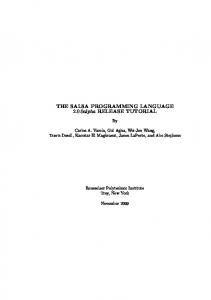
substituting x by its unique value, and v by successively all values in the set expression domain(x). 3.2. Composing choices In order to describe search algorithms, choices have to be composed. If C and D have been defined as two choices, the expression C×D represents the algorithm that first applies a transition from choice C and then applies a transition from choice D. In such a composition, C and D need not be different : one can apply the same branching mechanism over a whole search tree : Cn represent C composed n time with itself, and C* represents an infinite expression C×C×.... In the finite domain example, one can take decisions following the Inst choice until all variables are instantiated: such a strategy is described by the term Inst*: indeed, since the number of imbricate Inst choices required to instantiate all variables can be as large as the number of variables in FD.vars, a list of arbitrary length, the only expression that describes the desired search whatever the number of variables is the infinite term C×C×.... Note that if C generates no transitions, then C×D is also unable to branch; and C* either leads to infinite computations or ends up generating void alternatives. Another strategy would consist of reducing the domains by dichotomic splits until no more domains of size greater than 4 remain and then, applying the labeling procedure. Such an algorithm can be described as the composition of Split* and Inst*. However, it cannot be denoted Split*× Inst* since this expression would have to generate an infinite number of Split-transitions before performing the first Inst-transition. Hence, we introduce a new composition mechanism : if C and D are two choices C à D attempts to apply a transition of C; whenever C is unable to branch (when C does not manage to produce one single valid substitution by a tuple of values for its local variables, i.e. C generates 0 alternates), a transition of D is applied. Both composition mechanisms (× and à), are generalized to the composition of complex expressions involving choices. Thus, in our example, the new search procedure should be denoted Split*à Inst*, since it applies transitions from Split, and when it is no longer able to do so, it applies transitions from Inst, until it is no longer able to do so. Figure 1 shows the visual representation of the algorithm Split*à Inst*. A graphical syntax has been defined for SALSA. It bears similarities with flow charts and is enriched with a few search-specific conventions. Branching points are displayed with triangles. All such triangles have one incoming arrow at the top representing the entry point of the algorithm and may have two outgoing arrows: the arrow below the triangle base figures the control flow in each branch of the choice point; the outgoing arrow on the side of the triangle denotes the control flow whenever the choice is not able to branch. The bottom arrow is therefore a connector for ×–composition and the side arrow for à–composition. In both triangles of the example depicted figure 1, the bottom arrow goes back to the top of the triangle: this loop figures the C* construct which repeatedly applies transitions from a choice C until C is no longer able to branch.

7


start

Split end

Inst Figure 1: the graphical representation of a simple instantiation strategy for a finite domain CP engine: Split* à Inst*

There are two implicit rules for the visit of this diagram. First, when a failure occurs, the control backtracks to the father node (go up backwards the incoming top arrow), which, in turn, expands the next branch (follow the outgoing bottom arrow). Second, when all branches of a node have been explored, the control returns to the father node (go up backward the top arrow). 3.3 Running algorithms described by SALSA terms We have introduced above an example defining two choices. As a control mechanism, a choice leads from one state (a time instant during the computation) to a set of states (since there are several branches). The precise operational semantics of choices is defined in section 5, but we can consider as a first approximation that, if C is defined as follows : C :: Choice( moves f(x) with x ∈ g() )

then, the evaluation of C within state s yields the set of states {s1, ..., sn} if the evaluation of g() returns {x1, ..., xn} and if state si is obtained from state s by the evaluation of f(xi). A choice thus defines a neighborhood in the space of all states. In a standard implementation, these branches would be visited sequentially, one after the other. However, in order to account for distributed implementations of search algorithms, we leave unspecified the order of visit between these branches. In a sequential implementation, whenever a failure is detected in a branch, the algorithm « backtracks » (goes back to the father node, which, in turn, may either expand its next son, or, in case all of them have been visited, may backtrack to its own father node). In a distributed implementation, when a failure is detected, the node disappears (and informs its father of its death). A choice may actually have two different behaviors, either generating a non-empty set of decisions (a strict neighborhood of the current state), or generating an empty set of decisions (yielding an empty neighborhood). In the latter case, applying the choice has no effect: the system is said to have come to a fix-point for this choice. The two composition mechanisms are called leaf composition (×) and fix-point composition (à). Note that the construct C* describes this infinite composition of a choice with itself, until stability (fix-point state) is reached. The execution of such a term goes through a

8


search tree, in which some branches may be infinite. SALSA does not forbid nonterminating programs caused by infinite search trees. 3.4 Limitations Not everything can be done with SALSA: First, it is only a language for controlling (global, local and hybrid) search, therefore it is not a model for expressing solvers implementing various logic maintenance mechanisms. Second, as a control language, it also has its own limitations: -

SALSA’s computations are not continuations. The user cannot ask SALSA to resume

exploration from the previous solution, -

there is no way to express backjumping or intelligent backtracking methods,

-

the model handles one state at a time, so there is no way to express populationbased algorithms (genetic algorithms, scatter search, …).

4. Grammar This section presents a formal description of the language. We review SALSA’s grammar where we type in bold the reserved keywords and in italic the optional components. 4.1 Creating choices Choices are named objects that may be defined in a parametric manner (here, the parameters are x1,...,xi). (x1:,...,xi:) :: Choice( )

Grammar excerpt 1 : creating choices

A choice with free variables (x1,...,xi) is either directly defined with the moves keyword, an expression for defining the moves and a set of variable definitions, or it may use a case expression (conditional switch based on typing). The operational semantics requires that choice parameters (x1,...,xi) be fixed (no lazy evaluation) each time the choice is used to expand nodes in the search tree. ::= moves such that sorted by on failure ::= case ( , .... ) with

Grammar excerpt 2: defining choices

The set of moves considered for a choice can be defined in three ways :

9


-

either by a unique expression containing at least one free variable ranging over a set of values (defined in the with section)

-

or by explicit enumeration of the expressions to evaluate, separated by the or keyword,

-

or by an expression composing other choices, which we call a SALSA term. This last possibility is useful for looping over composite choices: since the expression (A×B)* is not valid, the trick is to create a new choice C, with moves from A× Β and to use C*.

::= post(,) post(,) or .... .... or post(,) from

| |

Grammar excerpt 3: defining moves

A choice thus corresponds to a set of moves, which can be processed in parallel. However, this set may then be modified by two optional lines in the choice definition. A first line (after such that) selects a subset of the moves. This can be done by stating any Boolean condition (which is tested before the move), or by using within a condition the expression delta(), which represent the variation of the numerical expression through the move1 (as in LOCALIZER). The second optional modification specifies the order in which these moves should be considered (a way of expressing value ordering heuristics). ::= | delta() ::=

Grammar excerpt 4: filtering moves

The structure of the section for defining the local variables xi+1,..., xn from the parameters x1,...,xi is described below. Note here that the expressions for defining the values of a variable may use mathematical expressions on sets such as {x in E | P(x)} (for subset selection), {f(x) | x in E} (for set image), some(x in E | P(x)) or some(x in E minimizing e(x)) (for the selection of an element in a set), etc. ::= with x1 , x2 , .... xn

Grammar excerpt 5: defining local variables

Choices can be combined together to form SALSA terms with the operators × … à … operator and a few other constructs defined in the next section.

1 : for instance, move flip(x) with x in S such that delta(cost) < -3 consider as valid alternates

flip(x) such that b-a>-3 where a and b are the value of cost, evaluated before and after the move (the evaluation of flip(x)).

10


4.2 Building Composite terms In order to complete the grammar, we give the syntax for the SALSA terms, which may be used either within choice definitions, or passed as parameters to the SOLVE primitive (this call is evaluated as a CLAIRE expression). ::=

| × à | / | ! | until | where | | ε

::=

* ( ,,,) × à

::=

∪ ∪x∈ ∈ ::=

| | | | | | |

cont | exit

::= SOLVE()

Grammar excerpt 6: using composed SALSA terms

The expression S × T1 à T2 (with S a SimpleTerm and T1, T2, SALSATerms) is not built by using two binary operators (it is neither S × (T1 à T2) nor (S× T1) à T2) but one ternary operator (it amounts to pretty printing for ×à (S,T1,T2)). ε is a special term denoting the empty term. In the remainder, we write S × T1 as a short cut for S × T1 à ε and S à T2 for S × ε à T2. Terminators specify the control flow when the search algorithm comes to an exit. There are two possible behaviors: either executing the whole algorithm described by the term until all nodes have come to an end (cont) or stopping the whole algorithm as soon as one state comes to an end (exit). Both terminators can be composed with a term either with à or ×. For instance, if C is a standard assignment choice (assigning one by one to a variable all values from its domain), C* à exit will search for solutions and stop at the first one encountered, whereas C* à cont will search for all solutions, but will return to the initial state of the system (the root node of the search tree) after the search has been performed. This last example, C* à cont, is, however, of little interest. Indeed, there is no way of knowing the number of solutions which have been encountered. One would like, to be able to do some printing or to update some global variables, in each fixpoint-exit of C*, before continuing the search. In order to offer such a possibility, the composition constructs, à and ×, are extended in order to accept as second argument functions as well as terms. The idea is to compose SALSA terms with functions which have side effects. For instance, if talk is a function that displays

11


some information about the current solution, the previous term can be replaced by C* à talk à cont, which evaluates talk() in all fix-point states generated by C*. The grammar also mentions the smallest primitive which denotes a look ahead search strategy which retains only the best exits. Let T be a term, f be a function of arity 0, n an integer and r a ratio between 0 and 100%. The execution of the term smallest(T,f,n,r) explores the search tree for T, evaluates f() in all its exits, computes the minimal value fmin of these evaluations, and goes back to those exits for which f() × r ≤ fmin , keeping at most n of them (the smallest ones)our2. For instance, if C is a choice, smallest(C,f,1,100%) goes into all branches of C, evaluates f(), and returns to one of the branches yielding the smallest value. A symmetrical primitive, largest, is also available. Unions of choices are introduced: C1∪C2 is the choice that applies all transitions from C1 and C2; Ux in E (C(x)) is the choice that yields all transitions of the choices C(x) for x in the set E. Topological conditions on the part of the tree that is visited may be expressed: -

The ‘/’ operator limits the number of exits of a term by an integer. As for smallest and largest, this applies only to terms having one single possibility for exiting : either leaf or fix-point. For example C* / 4 will behave like C* until the first four exits (fix-point exits) and will afterwards stop any further exploration (backtracking to the root node). Noe that the only difference between C* à exit and C* / 1 is that the second term can be further à–combined while the first cannot.

-

The ‘!’ operator limits the number of allowed backtracks in the tree. The execution of T ! n will be like that of term T until exactly n backtracks have been performed, in which case, the algorithm will stop any further exploration and backtrack to the root node for T.

The two last operators dynamically change the shape of the tree : -

in the term T where f, the where operator extracts from a given tree T, only those nodes n for which condition f() was satisfied all along the path from the root node to n. Note that this is a generalization to the case of arbitrarily complex SALSA expressions of the such that condition in the definition of one choice.

-

The until operator allows the user to express some conditions which should cause the search to stop, although the neighborhood has not yet been fully explored. In the term T until f, the until operator checks the condition f() at every inside node of T and performs the visit of T until an evaluation of f() yields true. Whenever f()=true, the algorithm by-passes the remainder of the search and exits with fixpoint state.

2 In order for thbis lookahead strategy to evaluate and compare f() in similar situations, an additional condition is imposed on T: it must be a term for which there is only one kind of possible exits, either leaf or fixpoint, but not both : for instance C*, C8 à cont, Cn × D* are such valid terms, whereas Cn, Cn à D* are not.

12


5. Operational Semantics We now present an operational semantics for SALSA: the evaluation of SALSA expressions is formally described by a set of transition rules in a calculus of distributed processes. A process is created each time a new node is expanded in the search tree. Processes have access to two different kinds of data : local data associated to the search node (for instance, the state of the domains in a CP solver, which differ from one node to the other) and global data which is used for communication between processes (for instance, in branch and bound optimization, the value of the best solution found so far, which is updated whenever a leaf is reached). Throughout the evaluation of a SALSA expression, the state of the system is described by a set of processes associated to the frontier of the tree (the limit between the part of the tree which has been explored and what has not yet been explored). Because of the communication through the global environment, processes are not independent. However, they are not implicitly synchronized and the exploration can follow any strategy (depth first, breadth first, or anything else). Thus, SALSA programs have nondeterministic behaviors: different runs of a same SALSA program may produce different results. For instance, a branch and bound optimization search may produce different sequences of solutions from one run to the other. SALSA specifies search algorithms systematically in a distributed environment, leaving aside the issues of load balancing and process priorities. In this respect, SALSA aims at two contradictory goals: specifying the control flow of an algorithm while retaining some declarativity. 5.1 The evaluation environment We first need to account for the evaluation of standard expressions of the host programming language. If the evaluation of the closed expression (without free variables) exp yields the value val, the evaluation will be denoted as :

(ξ , E ) : exp → (ξ ' , E ') : val The pair (ξ,E) denotes the state of the system, i.e. the set of existing objects, values of global variables, etc.... This evaluation environment of evaluation is separated in two parts : •

ξ is the global environment, shared by all processes

•

E is the local environment. Each process has its own version of this environment.

Both ξ and E may be changed by the evaluation in case of side effects. 5.2 Notation for choices and terms To keep the presentation simple, we assume that all choices are of the form

13


C :: Choice moves g(x) with x ∈ f() such that k() on failure h(x)

which we will denote by Choice(f,g,h,k). In fact, if f() returns an ordered list of tuples, any choice definition can be rewritten in such a form3. Such a choice definition is considered valid, if there exists a type X such that the functions f,g,h and k used in the choice definition meet the following conditions : 1. f is of type void → set[X], without side effects 2. g is of type X → {void, ⊥}, with allowed side effects on E 3. h is of type X → void, with allowed side effects on ξ and E 4. k is of type void → bool, without side effects. where ⊥ is a special value of the language, used for denoting failure. when these conditions are not met, the evaluation of the choice returns a typing error. After rewriting Cn as C×C..... ×C, C* as the infinite composition C×C×......, largest(T,f,…) as smallest(T,-f,…), and so on, one can reduce all SALSA terms to terms with the following binary (and possibly infinite) structure ::= × à

with ::=

Choice(,,,) | | ε | / | smallest(,,, )

5.3 Processes and transitions The semantics defines transitions of a system made of a global environment and a set of distributed processes. Processes are denoted as p : ℘ and have the following fields:

æ state : {start , expand , wait , done, failed }ö ç ÷ ç father : ℘ ÷ ÷ p : ℘ç sons : set[(< object >,℘)] ç ÷ ç env : set[< object >] ÷ ç code :< SALSATerm > ÷ è ø

3 This reduction isso mainly based on transforming nested loops into single iterations. For

instance moves g(x,y) with x∈ f1(), y∈ f2(x) is turned into moves G(X) with X ∈ F() with F() returning the list of pairs (x,y) such that x∈f1() and y∈f2(x) and G a function over pairs such that G((x,y))=g(x,y).

14


For such a process p, p.env is the environment of the process (E in the pair (ξ, E)), p.code is the remaining SALSA term to be evaluated from p and p.sons and p.father refer to related processes (with an obvious meaning in the search tree). In addition, we denote by π a newborne empty processes (different occurrences of π in the same expression actually denote different processes). The computation of the algorithm represented by the SALSA term will be represented by a sequence of transitions in the process algebra, according to the rules which follow. Transitions may change the number of pending processes as well as the global environment; they are written as: // (ξ ,{ p1 ,..., pn }) → (ξ ' ,{ p1 ' ,..., pl '})

where any processes pj’ is either distinct from the set of pi, or is one of the pi processes whose state has evolved. The latter case is denoted by: p j ' = p i [ field new value] For the sake of readability, transitions that update the state of one single process p will // // be written (ξ, p ) → (ξ', p[field /value]) instead of (ξ, p ) → (ξ',{p[field /value]}) 5.4 Transition rules in the process algebra We are now ready to state the rules specifying the legal transitions in this system. The rules should be read from bottom up. The transition below the horizontal line of the rule may be applied whenever all conditions above this line are satisfied.

The first rule links the evaluation of an expression solve(T) within the host programming language with the transitions in the process calculus: solve(T) will return either true or false, depending on the state of the final process; moreover, there may be side effects on the global environment (changed from ξ to ξ’) as well as on the local environment (changed from E to E’). p':℘(env= E') æ state=start ö ç ÷ p:℘ç env=E ÷ ç code=T ÷ è ø // (ξ, p) → (ξ', {p'})

( p'.state=done ∧ v=true)∨ ( p'.state= failed ∧ v=false) (ξ, E): solve(T) → (ξ', E'): v

Rule 1: link with the programming language

The second rule is the structural rule responsible for non-deterministic executions. It states that from a given frontier, any node can be expanded. One single process p may evolve into any number (n) of processes. Note however, that in order to avoid problems specific to parallelism (mutual exclusions, semaphores, etc.), we apply such transitions to only one such process p at a time.

15


// (ξ , p)  → (ξ , { p1 ' ,..., p n '}) // (ξ , {p, p1 ,..., p k })  → (ξ , {p1 ,..., pk , p1 ' ,..., p n '})

Rule 2: expanding one node of the frontier

Rules 3 and 4 start the evaluation of the choice, by generating the set of values for the variable in the lexical scope of the choice. Once this evaluation has been performed, the state of the choice is updated from start to expand and elementary processes are created for all sons of the current node (rule 3). In case an empty set of values was generated (rule 4), a fix-point exit is taken from the choice and the evaluation of the SALSA term moves on to T2.

ö æ state = start , env = E ÷÷ p :℘çç code Choice f g h k T T ( , , , ) = × à 1 2ø è (ξ , E ) : f () → (ξ , E ) : {x1 ,..., xn }, n > 0 state expand é ù // (ξ , p )  (ξ , p ê → ú) ë sons {( x1 ,π ),..., ( xn , π )}û Rule 3: expanding a node: generating the labels of the branches

æ state = start , env = E ö ÷÷ p :℘çç è code = Choice( f , g , h, k ) × T1 àT2 ø (ξ , E ) : f () → (ξ , E ) : {} // (ξ , p)  → (ξ , p[code T2 ]) Rule 4: generating an empty set of labels: fix-point exit

Rules 5 and 6 can be applied on all sons that have been generated by rule 3. In case the condition k() (after the such that keyword in the choice definition) is satisfied, rule 5 is applied: the transition g(xi) is evaluated in the ith branch of node p, and a new process p’ is added to the current frontier. In case the condition k() is not satisfied, or the transition (g(xi)) of the ith branch fails, rule 6 applies and the backward transition h(xi) is evaluated with side effects on the environment of node p. æ father = p, env = E ' ö ÷÷ p':℘çç è code = T1 , state = start ø ö æ state = expand , env = E ÷ ç p :℘ç code = Choice( f , g , h, k ) × T1 àT2 ÷ ç sons = {( x , p ),.., ( x , π ),.., ( x , p )}÷ 1 1 i n n ø è (ξ , E ) : k () → (ξ , E ) : true (ξ , E ) : g ( xi ) → (ξ , E ' ) : void // (ξ , p )  → (ξ , {p' , p[sons {( x1 , p1 ),..., ( xi , p' ),.., ( x n , pn )}]})

16


Rule 5: going down a branch

p':℘( father = p, state = failed ) æ state = expand , env = E ö ç ÷ p :℘ç code = Choice( f , g , h, k ) × T1àT2 ÷ ç sons = {( x , p ),..., ( x , π ),.., ( x , p )}÷ i n n ø 1 1 è

(ξ , E ) : g ( xi ) → (ξ , E ' ) : v (ξ , E ) : k () → (ξ , E ) : v'

(v = ⊥ ∨ v' =

false )

(ξ , E ) : h( xi ) → (ξ ' , E ' ' ) : void éenv E ' ' ù // (ξ , p )  → (ξ ' , p ê ú) ë sons {( x1 , p1 ),..., ( xi , p' ),.., ( x n , p n )}û Rule 6: failure in a branch

Rules 7, 8 and 9 apply when all sons of a node have been expanded and updates the state of the father node. By default, rule 7 updates its state from expand to wait value. In case all sons have reported a failure, rule 8 updates it from wait to failed, otherwise rule 9 updates it from wait to done.

æ state = expand ö ÷÷, ∀i, xi ≠ π p :℘çç è sons = {( x1 , p1 ),..., ( x n , p n )}ø // (ξ , p)  → (ξ , p[state wait ]) Rule 7: when all sons of a node have been expanded

∀i, pi .state = failed æ state = wait ö ÷÷ p :℘çç è sons = {( x1 , p1 ),..., ( xn , p n )}ø

// (ξ , {p, p1 ,..., p n , p1 ' ,..., pl '})  → (ξ ' , {p[state failed ], p1 ' ,..., pl '})

Rule 8: when all sons of a node report a failure

∀i ∈{2..n}, pi .state ∈ { failed , done} p1 .state = done æ state = wait ö ÷÷ p :℘çç è sons = {( x1 , p1 ),..., ( xn , p n )}ø

// (ξ , {p, p1 ,..., p n , p1 ' ,..., pl '})  → (ξ ' , {p[state done], p1 ' ,..., pl '})

Rule 9: when all sons of a node have finished their computations

Rules 10 and 11 apply when one of the processes (say p1) has to evaluate (in its code field) a terminator. In the case of the exit terminator, rule 10 discards all other

17


processes in the frontier, otherwise, rule 11 discards the process p1. Note that these rules 10 and 11 are different from all the other ones since they apply on the whole frontier and not only on one single node. Therefore, they perform an explicit synchronization between a set of processes. p1 .code = exit // (ξ , {p1 ,..., pn })  → (ξ ' , {p1 [state done]}) Rule 10: exit terminator

p1 .code = cont // (ξ , {p1 ,..., pn })  → (ξ ' , {p 2 ,..., p n }) Rule 11: cont terminator

Rule 12 specifies the evaluation of a SALSA term T/n within a process p. The evaluation rules are applied on T within a clone process p’ of p. The process p’ evolves into a search tree frontier. We consider those processes pi in the frontier which have been fully evaluated (such that pi.code = ε) and that have not failed (such that pi.state = start). Whenever a state is reached with n such processes, or with less than n, but no hope to generate any further ones, these very processes are kept and all other ones are dismissed. The SALSA code to evaluate is moved on to T1 for these processes. p':℘(state = start , env = E , code = T ) p :℘(state = start , env = E , code = T / n × T1 àT2 ) æm = n ö ç æm < n ö÷ ç∨ ç ÷÷ ç ç ∀j ∈ {1..l}, p j '.code ≠ ε ∧ p j '.state ∈ { failed , done, wait} ÷ ÷ øø è è // (ξ , p' )  → (ξ ' , {p1 ,..., p m , p1 ' ,..., pl '}, m > 0

(

)

∀i ∈ {1..m}, ( pi .state = start , pi .code = ε ) // (ξ , p)  → (ξ ' , {p1 [code T1 ],..., p m [code T1 ]}) Rule 12: limiting the number of exits of a search

Rule 13 specifies the evaluation of a SALSA term smallest(T,f,n,r) within a process p. The evaluation rules are applied on T within a clone process p’ of p, until all processes are either internal nodes or failed leaves (processes pj such that pj.state ∈ {wait, failed, done}) or successful leaves (processes pi such that pi.code = ε). The heuristic f() is evaluated in each successful leaf and they are sorted by increasing values. Only the leaves with the smallest values are kept. We keep at most n of them, and retain only those which are above the ratio r compared to the best one. From those best k processes, the SALSA term T1 is evaluated.

18


p':℘(state=start,env=E,code=T ) æ state=start,env= E ö ÷÷ p:℘çç è code=smallest(T, f,n,r)×T1àT2 ø (ξ, p) →// (ξ', {p1,..., pm, p1',..., pl'}, m>0 ∀i∈{1..m}, ( pi.state=start, pi.code=ε ) ∀j∈{1..l}, ( p j.state∈{wait, failed,done}) ∀i∈{1..m}, (ξ, pi.env): f() →(ξ, pi.env):ai a1≤a2 ≤...≤am q=min(i∈{1..m} | ai >a1/ r ) k =min(m,n,q) // (ξ, p) → (ξ', {p1[code T1],..., pm[code T1]}) Rule 13: look-ahead search

Rule 14 specifies the evaluation of terms T/n or smallest(T,f,n,r) when the first exploration (in the process p’ cloned from p) fails. In this case, the process evaluating C comes to a fix-point exit and term T2 is evaluated. p':℘(state = start , env = E , code = T ) æ state = start , env = E ö ÷÷ p :℘çç è code = C × T1 àT2 ø C = T / n ∨ C = smallest (T , f , n, r )

// (ξ , p' )  → (ξ ' , {p' '}), p' '.state = failed // (ξ , p)  → (ξ ' , {p' ' [code T2 , state start ]})

Rule 14: no exits from a look-ahead or limited search

A proprietary prototype has been implemented at Thomson/CSF after this semantics. It is implemented as a code generator : SALSA expressions are expanded into CLAIRE code, which, in turn is compiled into C++ code. On average, one line of SALSA generates 10-15 lines of CLAIRE which, in turn, generate about 50-100 lines of C++. The other possibility would have been to implement an interpreter. Although technically simpler, this would have implied a run-time overhead in the code. Such an overhead is acceptable for global search algorithms performing much work in each node (such as branch and cut algorithms or CP with global constraints). However, the run-time interpretation of control structures induces a penalty for “light-weight” local search algorithms. The concern for efficiency motivated the compile vs. interpret decision. Note that other tools such as Ilog parallel solver [Pe 99] (focused on global search for CP), or LOCALIZER [MVH 97] (featuring rich invariant language but simpler control structures) settled for the interpreted approach.

6. Examples This section is devoted to the illustration of the SALSA language on examples in combinatorial optimization :

19


1.

A simple customized procedure for a combinatorial toy problem: placing queens on a chessboard.

2.

A standard local optimization algorithm, GSAT. This example was already discussed with LOCALIZER; we show how the SALSA formulation is a natural extension of the LOCALIZER approach.

3.

Experiments with greedy heuristics and limited backtracking on a simple scheduling problem.

4.

Lin & Kernighan's heuristic for the traveling salesman problem (TSP), in which the search for the best local moves is done by a global search algorithm.

5.

Hybrid algorithms for vehicle routing problems. These algorithms combine various forms of local optimization, look-ahead evaluation, greedy heuristics and constraint propagation.

6.1 The n queens problem

How should be placed n queens on an n×n chessboard, such that no two of them attack each other ? We model this problem in CP with an array, named queens, of finite domain variables : queens[i]=j means that there is a queen in the cell at the intersection of line i and row j). We denote by FD the solver constraining the rows and diagonals of the various queens to be different. A useful heuristic consists in selecting the variable on which to branch by the first-fail criterion and iterating the values in its domain, starting from the center of the row [Jou 95]. Such a branching procedure can be described by a SALSA choice which sorts the tuples of values for its local variables (i and j) by increasing distance to the middle of the row. Q :: Choice( moves post(FD, queens[i] == j) with i = some(i1 in {i0 in (1 .. n) | unknown(value,queens[i0])} minimizing card(domain(queens[i1])) ) j ∈ domain(i) sorted by increasing abs(n/2 - j))

We can now easily describe an algorithm which looks for all solutions and displays them all by calling each time the display function. This algorithms is described by the term Q* à display à cont and is represented in figure 2. start display

Q

Figure 2: the graphical representation of a search algorithm displaying all solutions to the n-queens problem

20


6.2 GSAT We now focus on a famous example from local optimization. The GSAT algorithm was proposed in [SLM 92] in order to solve the 3-SAT problem. Such a problem is defined by a set of Boolean variables and a set of clauses which are conjunctions of three literals (variables or negations of variables). The problem consists in finding an assignment of values to variables such that all clauses are satisfied. The algorithm starts with a random assignment and flips some variables (changing them to their opposite value). The algorithm tries to repair the solution by performing those flips that decrease the number of violated clauses). Such a local move can thus easily be described by : SimpleFlip :: Choice( moves x.value := not(x.value) with x = some(x in Litteral | exists(c in Clause | involves(c,x) & unsatisfied(c)) such that delta(card({c in Clause | unsatisfied(c)}) 1 & l[1] = l[length(l)]) )

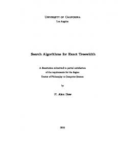
The global search algorithm for finding one local move, as it is proposed in the original paper [LK 73], backtracks on the first two levels of the search tree (considering all possibilities for the two first vertices of l), and from then on, only considers the addition of the vertex yielding maximal gain. It can thus be described as follows : SOLVE(largest(Init × Augment × largest(Augment,gain,1,100%)*, gain, 1 ))

Once the best move has been found, we can perform it (flipping the edges along the alternating cycle) by calling the performMove function. The full algorithm is a standard hill-climbing procedure which applies such local moves until no more improvement can be made and can be easily specified on figure 8 : start

Init

Augment end

Augment 1 gain 1 gain

1

performMove

Figure 8: the Lin and Kernighan heuristic:

26


SOLVE(largest(Init × Augment × largest(Augment,gain,1,100%)*, gain, 1, 100%) × performMove)* à exit)

Hence, using SALSA, we have proposed a simple description of a well-known complex algorithm. Moreover, with such a description, it is easy to experiment with variations of this algorithm. For instance, the algorithm can be modified in order to generate more than one single move in each neighborhood (say, at most 3) and to backtrack on all possible sequences of such favorite moves. In order to generate a set of such good moves, we not only fully branch on all possible starts for the alternate cycle (Init), but we also keep two branches for the two next nodes in the cycle (Augment/2)2. Such a variation on the original Lin and Kernighan procedure is proposed in figure 9.

start

Init

Augment ≤2

2

Augment 1 gain 1 95%

100%

gain

dist

3

1

end Figure 9: a variation on the Lin and Kernighan heuristic: SOLVE(smallest( largest(Init × (Augment/2)2 × largest(Augment,gain,1,100%)*, gain, 3, 95%)*, dist, 1, 100%) à exit)

Table 3 relates a few experiments comparing both algorithms. For 5 random 50-node instances, we report the objective value (the length of the tour) returned by a greedy heuristic, and the value and running times on a Sun Sparc 10 returned by both

27


algorithms. As expected, the variation which performs more global search slows down the algorithm and improves the quality of solutions4. Greedy

LK

Customized LK

pb1

1008

846 15s.

844 58s.

pb2

922

814 14s.

740 40s.

pb3

880

866 4s.

866 5s.

pb4

868

704 16s.

704 80s.

pb5

1004

920 16s.

888 56s.

Table 3: variations on the Lin and Kernighan heuristic 6.5 Hybrid insertion heuristics for vehicle routing This last example is devoted to hybrid algorithms for vehicle routing problems, which combine local and global search. Vehicle routing problems can be stated as follows : given a set of customers and a central depot, find a set of routes covering all customers, each route starting and ending in the depot, and respecting some side constraints (limited route length, limited amount of goods transported along a route, time windows, etc.). The objective is to find a solution with minimal total length. Insertion algorithms start with empty routes, select the tasks one by one and insert them into a route. Such algorithms are widely used heuristics in practical routing software because they are able to handle many additional constraints. Their performance can be significantly improved if a limited amount of local optimization is performed after each insertion [GHL 94], [Ru 95], [CL 99a]. This leads to a complex algorithm using global search as a general framework (a greedy heuristic with a limited look-ahead exploration of the branches for each insertion), and using local search at each node of the search tree. We show here how SALSA can be used to program a simplified version of this algorithm; and refer the reader to [CL 99a] for more details.

We start by describing the simple greedy heuristic. Inserting a customer c in a route r can be described as a choice. We consider all pairs of adjacent vertices (x,y) in r and try to insert c between x and y by posting to the dispatch solver the information that x and c are now linked by an edge in the route r as well as c and y. Note that the Insert choice is defined with two parameters, c and r.

4 The results are pessimistic in running times as well as quality of solution, compared to

[LK73]. This is due to the fact that our implementation works for asymmetrical TSP’s as well as symmetrical ones. In order to adapt to the asymmetrical case, we considered only moves which do not reverse the visit order of a sub-chain in the tour. Moreover, some cuts from the symmetrical case do not apply.

28


Insert(c:Customer, r:Route) :: Choice( moves post(dispatch, (link(x,c,r), link(c,y,r))) with (x,y) ∈ edges(r) sorted by increasing insertionCost(c,x,y) )

From such a choice, we only retain the edge (x,y) with the least insertion cost, by limiting the number of branches to 1 (since the branches are sorted by increasing insertion costs). While inserting one customer c, we only keep, for each route, the best possible insertion place: this is described by keeping for each route r, only one branch of the choice Insert(c,r) and taking the union of these choices for all routes r. Insert(c:Customer) :: Choice( moves from ∪r ∈ Routes(Insert(c,r) / 1) )

Among all these possibilities of insertion, we select only the one yielding the minimal total cost5. OneInsert :: Choice( moves from smallest(Insert(c), TotalLength(), 1) with c = some(c0 in Customer | unassigned(c0)) )

The greedy algorithm can hence be described as follows : SOLVE(OneInsert* à exit)

We now come to incremental local optimization, which will be performed after each insertion. Below, we describe two choices responsible for local moves. The first choice is responsible for a 2-opt local move on the route to which t belongs (2-opt is a standard optimization procedure for routing problems which erases 2 edges xy and uz from a route, replaces them by the edges (x,u) and (y,z) and reverses the links between y and u). The second choice is responsible for a 3-opt optimization which concerns edges from 2 or 3 different routes: we replace the edges (t,u), (x,y) and (z,w) by (x,u), (z,y) and (t,w). Both kinds of local moves, are accepted only when they yield an improvement in the total length of the solution. TwoOpt(c:Customer) :: Choice( moves post(dispatch, ( link(x,u,r), link(y,z,r), reverse(y,u,r)) ) with r = route(c), ((x,y), (u,z)) ∈ SortedPairsOf(edges(r)) such that delta(Length(r)) < 0 ) ThreeOpt(c:Customer) :: Choice( moves post(dispatch, ( link(x,u,r1), link(z,y,r2), link(c,w,r))) with r = route(c), u = next(c), r1 ∈ RoutesCloseTo(r), r2 ∈ RoutesCloseTo(r), (x,y) ∈ edges(r1), (z,w) ∈ edges(r2) such that delta(TotalLength) < 0 )

We can now describe an enriched version of the heuristic which performs a limited amount of local optimization during the insertion : for each route r, after having found 5 Recall that the expression some(x in S | P(x)) returns one single element from S such that

P(x)=true.

29


the best pair of points between which c should be inserted and before evaluating the insertion cost, we perform at most n steps of 2-opt in order to optimize r. This enables us to perform a more informed choice among all possible insertions. Then, once the best insertion has been chosen and performed, we further optimize the solution by performing at most m steps of 3-opt optimization, which may recombine the route in which the task has been inserted with other routes. SmartInsert:: Choice( moves from smallest(Insert(c) × (TwoOpt(c)/1)n,TotalLength(),1,0%) × (ThreeOpt(c)/1)m with c = some(c0 in Customer | unassigned(c0)) )

The final greedy procedure6 can then be described as SOLVE((SmartInsert/1)* à exit)

We have just described here, with 25 lines of SALSA code a hybrid algorithm for vehicle routing. By looking from top down at this specification, one can see that it is a greedy algorithm (it is of the form C/1*), that the basic step performs a look-ahead exploration of a choice, and that the basic choice uses various moves and hillclimbing random walks. Compared to an imperative implementation of such a hybrid algorithm, it is much more concise and it gives a global view of the algorithm, which is useful for understanding what the algorithm does. This SALSA code is independent from the data structures, the consistency mechanisms, as well as the computation environment (distributed or sequential). It is thus a high-level description of the control of the algorithm, complementary with a logic statement of the problem.

7. Future directions This paper has introduced a language for describing complex algorithms in combinatorial optimization with small terms. We have shown that one of the advantages of such descriptions is to act as brainteasers and to suggest to the programmer possibilities of variations over the original idea. This creative process of algorithm tuning can be performed more systematically: in a companion paper [CLS 99], we propose to apply a simple learning scheme in order to discover interesting algorithms for vehicle routing problems. This learning process is used in order to tune an algorithm to a set of instances, to a target run-time, or to a modified objective function. The algorithms are expressed in a variant of SALSA specialized for vehicle routing problems: this amounts to using pre-defined choices and letting the learner recombine them in whatever way he wishes. The results show that the approach is worthwhile and that the learner is able to discover new algorithms that significantly improve over hand-made combinations of insertion, local optimization and global search. Another range of application for the automatic tuning of algorithms to a problem and a computation environment is the case of real-time on-line optimization. [DGS99]

6 This greedy procedure is further enriched, with a limited forms of branching in [CL99a].

Such algorithms could be described as richer SALSA terms over the same basic choices. We refer the reader to [CL99a] for a detailed study with experiments and run-time figures.

30


presents a set of experiments with SALSA where a parametric optimization algorithm is used for which the parameters are tuned on-line, during the execution. This yields a new kind of self-adaptive optimization software. The amount of backtracking, the level of local optimization, the version of the algorithm used for computing bounds, all those parameters may be tuned before hand by a gross estimate on the difficulty of the instance. They can be updated and refined at run time, depending on the part of the optimization that has already taken place. Such a behavior is particularly interesting in the case of anytime optimization [Zi 93], where one tries to use the best algorithm for a given time contract. Note that the idea of tuning a search algorithm to a given problem and computation environment is also addressed in [LL 98], with the idea of search tree sampling.

8. Conclusion In this paper, we have presented SALSA, a language for programming search algorithms. We have proposed an operational semantics and have used the language to describe algorithms for combinatorial optimization problems. These algorithms relate to constraint programming and global search, local optimization and random walks or hybrid combinations of greedy constructive heuristics, local and global search. A few experiments have been reported with a prototype SALSA compiler. In the quest for general models and tools for operations research, SALSA is the first unified language for local and global search algorithms. Among the proposals for combining those two antagonistic paradigms [PG 96], SALSA offers a common formalism focused on control. The availability of a common language for global and local search algorithms is an interesting asset for the design of hybrid algorithms. On the examples that have been proposed, the SALSA code yields a concise specification of the control of the algorithm. Hence, SALSA is a step in the quest for elegant and declarative descriptions of complex algorithms. In addition, the compiler gives the programmer the ability to easily experiment with many variations of an algorithm, which is valuable for experimenting new ideas or tuning hybrid algorithms. The past years have seen the rise of interest for optimization tools with the introduction of tools dedicated to global search (Oz explorer [Sch 97], Ilog Parallel solver [Pe 99], visual CHIP [SA 99]), column generation (LP Shift/Roster [ED 99], Xpress cut pool manager [TB 98], Parrot [JK+99]) or scripts for optimization components (OPL studio [VH 99]). If, as J.-F. Puget puts it, “Constraint Programming is Software Engineering applied to Operations Research” [Pu 99], then, Operations Research analysts should use two kinds of tools: •

Components applying well-known techniques to well-known problems. Such tools may include specific models, solvers, agent systems, truth maintenance systems, blackboards, etc. These components state what problem is solved and how it is going to be solved.

•

A toolbox for combining such algorithmic components. With such languages, the programmer would state how the tools are coordinated in order to solve the problem.

31


SALSA is a tool of the second kind. Our experiments with SALSA for modeling existing algorithms (such as Lin and Kernighan’s heuristic) as well as our experiments for discovering new ones (with the automatic learner) indicate that this is a promising software engineering direction.

Acknowledgments The prototype SALSA compiler was developed at the Thomson-CSF Corporate Laboratories. We would like to thank Éric Bourreau, Simon De Givry, Éric Jacopin, Juliette Mattioli, Laurent Perron, Jean-François Puget and Benoît Rottembourg for fruitful discussions.

References [AS 97]

K.R. Apt, A. Schaerf, Search and Imperative Programming, Proc. POPL’97, ACM Press, 1997

[Be 00]

N. Beldiceanu, Global constraints as graph properties on structured nework of elementary constraints of the same type, technical report T2000-01, SICS, 2000.

[BV 98]

E. Balas, A. Vazacopoulos. Guided Local Search with Shifting Bottleneck for Job Shop Scheduling, Management Science, vol 44, n° 2, 1998.

[CL 99a]

Y. Caseau, F. Laburthe. Effective Forget and Extend Heuristics for Scheduling Problems, 3rd Metaheuristics International Conference, 1999.

[CL 99b]

Y. Caseau, F. Laburthe. Heuristics for Large Constrained Vehicle Routing Problems, Journal of Heuristics 5(3), p.281-303, 1999.

[CLS 99]

Y. Caseau, F. Laburthe, G. Silverstein. A Meta-Heuristics Factory for Vehicle Routing Problems, proc. of CP’99, J. Jaffar ed., LNCS 1713, Springer, 1999.

[DGS 99]

S. De Givry, P. Savéant. Optimisation Combinatoire en Temps Limité: Depth First Branch and Bound adaptatif, proc. of JFPLC’99, F. Fages ed., Hermes Science Publication, 1999.

[DT 93]

M. Dell’Amico, M. Trubian. Applying Tabu-Search to the Job-Shop Scheduling Problem. Annals of Op. Research, 41, p. 231-252, 1993.

[De 92]

E. Demeulemeester. Optimal Algorithms for various classes of multiple resource constrained project scheduling problems, PhD. dissertation, Université Catholique de Louvain, Belgium, 1992.

[ED 99]

LP Shift and LP Roster documentation, http://www.eurodecision.fr

[FMK 93] R. Fourer, D. MacGay, B.W. Kernighan. AMPL: A Modelling Language for Mathematical Programming, Brook/Cole Publishing Company, 1993. [GHL94]

M. Gendreau, A. Hertz, G. Laporte. A Tabu Search Heuristic for the Vehicle Routing Problem, Management Science, 40, p. 1276-1290, 1994.

[He 87]

R. Helm. Inductive and Deductive Control of Logic Programs, Proc. of ICLP 87, p. 488-512, 1987.

32


[HG 95]

W. Harvey, M. Ginsberg. Limited Discrepancy Search, Proceedings of the 14th IJCAI, p. 607-615, Morgan Kaufmann, 1995.

[HS 98]

M. Hanus, F. Steiner. Controlling Search in Declarative Programs, PLIP/ALP, p. 374-390, 1998.

[JL 87]

J. Jaffar, J.-L. Lassez. Constraint Logic Programming, Proceedings of the ACM symposium on Principles of Programming Languages, 1987.

[Jou 95]

J. Jourdan. Concurrence et Coopération de Modèles Multiples dans les Langages CLP et CC, PhD thesis, University of Paris 7, 1995.

[JK+ 99]

U. Junker, S. Karish, N. Kohl, B. Vaaben, T. Fahle, M. Sellmann. A Framework for Constraint Programming Based Column Generation, proc. of CP’99, J. Jaffar ed., LNCS 1713, Springer, 1999.

[Ko 79]

R.A. Kowalski: Algorithm = Logic + Control, CACM 22(7) p.424-436, 1979.

[LK 73]

S. Lin, B.W. Kernighan. An Effective Heuristic for the Traveling Salesman Problem. Operations Research 21, 1973.

[LL 98]

L. Lobjois, M. Lemaître. Branch and Bound Algorithm Selection by Performance Prediction, in Proc. of AAAI’98, Madison, WI, USA, 1998.

[Llo 87]

J.W. Lloyd. Foundation of Logic Programming, Springer, 1987.

[MS 96]

D. Martin, P. Shmoys. A time-based approach to the Jobshop problem, Proc. of IPCO'5, M. Queyranne ed., LCNS 1084, Springer, 1996.

[MVH 97] L. Michel, P. Van Hentenryck. Localizer: A Modeling Language for Local Search. Proc. of CP'97, LNCS 1330, Springer, 1997. [MH 97]

N. Mladenovic, P. Hansen. Variable Neighborhood Search, Computers Oper. Res. 24, p. 1097-1100, 1997.

[Na 84]

L. Naish. Heterogeneous SLD resolution, Journal of Logic Programming 1(4) p. 297-303, 1984.

[Pea 84]

J. Pearl. Heuristics: Intelligent Search Strategies for Computer Problem Solving, Addison-Wesley, 1984.

[Pe 99]

L. Perron. Search Procedures and Parallelism in Constraint Programming, proc. of CP’99, J. Jaffar ed., LNCS 1713, Springer, 1999.

[PG 96]

G. Pesant, M. Gendreau. A View of Local Search in Constraint Programming, proc. of CP'96, LNCS 1118, p. 353-366, Springer 1996.

[Pu 99]

J.-F. Puget. Constraint Programming: a Framework for Mathematical Programming, invited lecture, CP-AI-OR workshop, Ferrara 1999.

[Ru 95]

R. Russell. Hybrid Heuristics for the Vehicle Routing Problem with Time Windows, Transportation Science, 29 (2), may 1995.

[SS 94]

C. Schulte, G. Smolka. Encapsulated Search for Higher-order Concurrent Constraint Programming, Proc. of ILPS'94, p. 505-520, MIT Press, 1994.

33


[Sch 97]

C. Schulte. Oz explorer: A Visual Constraint Programming Tool, Proc. 14th ICLP, L. Naish ed., p. 286-300, MIT Press, 1997.

[SLM 92]

B. Selman, H. Levesque, D. Mitchell. A New Method for Solving Hard Satisfiability Problems Proc. of AAAI-92, p. 440-446, 1992.

[Sh 98]

P. Shaw. Using Constraint Programming and Local Search Methods to Solve Vehicle Routing Problems, proc. of CP’98, LNCS 1520, Springer, 1998.

[SA 99]

H. Simonis, A. Aggoun. Search Tree Debugging, proc. of JFPLC’99, F. Fages ed., Hermes Science Publication, 1999.

[TB 98]

J. Tetboth, R. Daniel, A Tightly Integrated Modelling and Optimisation Library : a new Framework for Rapid Algorithm Development, submitted for publication, 1998.

[VH 99]

P. Van Hentenryck. The OPL Optimization Programming Language, MIT Press, 1999.

[Zi 93]

S. Zilberstein. Operational Rationality through Compilation of Anytime Algorithms, PhD. dissertation, University of California at Berkeley, 1993.

34

SALSA: A Language for Search Algorithms

SALSA: A Language for Search Algorithms

Suggest Documents