sample-level deep convolutional neural networks for music auto ...

SAMPLE-LEVEL DEEP CONVOLUTIONAL NEURAL NETWORKS FOR MUSIC AUTO-TAGGING USING RAW WAVEFORMS Jongpil Lee Jiyoung Park Keunhyoung Luke Kim Juhan Nam Korea Advanced Institute of Science and Technology (KAIST) [richter, jypark527, dilu, juhannam]@kaist.ac.kr

arXiv:1703.01789v1 [cs.SD] 6 Mar 2017

ABSTRACT Recently, the end-to-end approach that learns hierarchical representations from raw data using deep convolutional neural networks has been successfully explored in the image, text and speech domains. This approach was applied to musical signals as well but has been not fully explored yet. To this end, we propose sample-level deep convolutional neural networks which learn representations from very small grains of waveforms (e.g. 2 or 3 samples) beyond typical frame-level input representations. This allows the networks to hierarchically learn filters that are sensitive to log-scaled frequency, such as mel-frequency spectrogram that is widely used in music classification systems. It also helps learning high-level abstraction of music by increasing the depth of layers. We show how deep architectures with sample-level filters improve the accuracy in music auto-tagging and they provide results that are comparable to previous state-of-the-art performances for the Magnatagatune dataset and Million song dataset. In addition, we visualize filters learned in a sample-level DCNN in each layer to identify hierarchically learned features. 1. INTRODUCTION In music information retrieval (MIR) tasks, raw waveforms of music signals are generally converted to a time-frequency representation and used as input to the system. The majority of MIR systems use a log-scaled representation in frequency such as mel-spectrograms and constant-Q transforms and then compress the amplitude with a log scale. The time-frequency representations are often transformed further into more compact forms of audio features depending on the task. All of these processes are designed based on acoustic knowledge or engineering efforts. Recent advances in deep learning, especially the development of deep convolutional neural networks (DCNN), made it possible to learn the entire hierarchical representations from the raw input data, thereby minimizing the input data processing by hands. This end-to-end hierarchical learning was attempted early in the image domain, particularly since the DCNN achieves break-through results in image classification [1]. These days, the method of stacking small filters (e.g. 3x3) is widely used after it has c 2017 Jongpil Lee et al. This is an open-access article distributed Copyright: under the terms of the Creative Commons Attribution 3.0 Unported License, which permits unrestricted use, distribution, and reproduction in any medium, provided the original author and source are credited.

been found to be effective in learning more complex hierarchical filters while conserving receptive fields [2]. In the text domain, the language model typically consists of two steps: word embedding and word-level learning. While word embedding plays a very important role in language processing [3], it has limitations in that it is learned independently from the system. Recent work using CNNs that take character-level text as input showed that the end-toend learning approach can yield comparable results to the word-level learning system [4, 5]. In the audio domain, learning from raw audio has been explored mainly in the automatic speech recognition task [6–10]. They reported that the performance can be similar to or even superior to that of the models using spectral-based features as input. This end-to-end learning approach has been applied to music classification tasks as well [11, 12]. In particular, Dieleman and Schrauwen used raw waveforms as input of CNN models for music auto-tagging task and attempted to achieve comparable results to those using mel-spectrograms as input [11]. Unfortunately, they failed to do so and attributed the result to three reasons. First, their CNN models were not sufficiently expressive (e.g. a small number of layers and filters) to learn the complex structure of polyphonic music. Second, they could not find an appropriate non-linearity function that can replace the log-based amplitude compression in mel-spectrograms. Third, the bottom layer in the networks takes raw waveforms in frame-level which are typically several hundred samples long. The filters in the bottom layer should learn all possible phase variations of periodic waveforms which are likely to be prevalent in musical signals. The phase variations within a frame (i.e. time shift of periodic waveforms) are actually removed in mel-spectrograms. In this paper, we address these issues with sample-level DCNN. What we mean by “sample-level” is that the filter size in the bottom layer may go down to several samples long. We assume that this small granularity is analogous to pixel-level in image or character-level in text. We show the effectiveness of the sample-level DCNN in music auto-tagging task by decreasing strides of the first convolutional layer from frame-level to sample-level and accordingly increasing the depth of layers. Our experiments show that the depth of architecture with samplelevel filters is proportional to the accuracy and also the architecture achieves results comparable to previous stateof-the-art performances for the Magnatagatune dataset and the Million song dataset. In addition, we visualize filters learned in the sample-level DCNN.

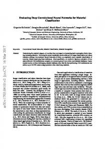
Frame-level mel-spectrogram model

Frame-level raw waveform model

Mel-spectrogram extraction

Frame-level strided convolution layer

Sample-level raw waveform model

Sample-level strided convolution layer

Figure 1. Simplified model comparison of frame-level approach using mel-spectrogram (left), frame-level approach using raw waveforms (middle) and sample-level approach using raw waveforms (right). 2. RELATED WORK Since the waveform is one-dimensional data, previous work use a CNN that consists of one-dimensional convolution and pooling stages. While the convolution operation and filter length in upper layers are usually similar to those used in the image domain, the bottom layer that takes waveform directly conducted a special operation called strided convolution, which takes a large filter length and strides it as much as the filter length (or the half). This frame-level approach is comparable to sliding windows with 100% or 50% hop size in short-time Fourier transform. In many of previous work, the stride and filter length of the first convolution layer was set to 10-20 ms (160-320 samples at 16 kHz audio) [8, 10–12]. In this paper, we reduce the filter length and stride of the first convolution layer to sample-level, which can be as small as 2 samples. Accordingly, we increase the depth of layers in the CNN model. There are some works that use 0.6 ms (10 samples at 16 kHz audio) as a stride length [6, 7], but they used a CNN model only with three convolution layers, which is not sufficient to learn the complex structure of musical signals.

3. LEARNING MODELS Figure 1 illustrates three CNN-based models in the music auto-tagging task we compare in our experiments. In this section, we describe the three models in detail.

3.1 Frame-level mel-spectrogram based model This is the most common CNN model used in music autotagging. Since the time-frequency representation is two dimensional data, previous work regarded it as either twodimensional images or one-dimensional sequence of vectors [11, 13–15]. We only used one-dimensional(1D) CNN model for experimental comparisons in our work because the performance gap between 1D and 2D models is not significant and 1D model can be directly compared to models using raw waveforms.

3.2 Frame-level raw waveform based model In the frame-level raw waveform-based model, a strided convolution layer is added beneath the bottom layer of the frame-level mel-spectrogram based model. The strided convolution layer learns a filter-bank represention that correspond to filter kernels in a time-frequency representation. In this model, once the raw waveforms pass through the first strided convolution layer, the output feature map has the same dimensions as the mel-spectrogram. This is because the stride, filter length, and number of filters of the first convolution layer correspond to the hop size, window size, and number of mel-bands in the mel-spectrogram, respectively. This configuration was used for music autotagging task in [11, 12] and so we used it as a baseline model. 3.3 Sample-level raw waveform based model As described in Section 1, the approach using the raw waveforms should be able to address log-scale amplitude compression and phase-invariance. Simple adding a strided convolution layer is not sufficient to overcome the problems. To improve this, we add multiple layers beneath the frame-level layer such that the first convolution layer can handle much smaller length of samples in filter length. For example, if the stride of the first convolution layer is reduced from 729 to 243, 3-size convolution layer and maxpooling layer are added to keep the output dimensions in the subsequent convolution layers equal. If we go down deep into sample-level along this framework, Six convolution layers (five pairs of 3-size convolution and maxpooling layer following one 3-size strided convolution layer). This is because the temporal dimensionality reduction occurs only through max-pooling and striding when zeropadding is applied on convolution layer to conserve input and output dimensions. We describe the configuration strategy of sample-level CNN model in the following section. 3.4 Model Design Since the length of an audio clip is variable in general, the following issues should be considered when configuring the temporal CNN architecture:

• Convolution filter length and sub-sampling length. • The remaining temporal dimension after the last subsampling layer. • The segment length of audio corresponding to the input size of the network. First, we attempted a very small (sample-level) filter length in convolutional layers by referring to the VGG net [2]. However, unlike images with spatial dimensions such as 224 × 224, audio files contains, for example, 22050 samples per second. Total input size may be similar with images if we use 2.3 seconds of audio as input to the network (224 × 224 ' 22050 × 2.3). However, since we use one-dimentional convolution and sub-sampling for raw waveforms, the filter length and pooling length need to be varied. Therefore, we constructed several different DCNN models to verify the effects on music auto-tagging performance. As a sub-sampling method, max-pooling is generally used. Although sub-sampling using strided convolution has recently been proposed in generative model [9], our preliminary test showed that max-pooling was superior to the stride-style sub-sampling method. We assume that this result is due to the high density characteristics of music data and translation invariance characteristics, which is the advantage of using max-pooling in classification tasks. Thus, we used max-pooling as the basic sub-sampling method. In addition, to test the model performance with minimum layer setting, a pair of single convolution layer and maxpooling layer that share the same filter length and pooling length was defined as a basic building module of the DCNN. Second, the remaining time dimension after the last subsampling layer represents the temporal compression ratio of the entire input audio. We set this value to one in all models in order to compare the performance according to the depth of layers and the stride of first convolution layer. The dimension of the fully connected layer that follows after the last sub-sampling layer is closely related to this value. By shortening this value to one, the parameter can be stored and the fully connected layer can be replaced by a convolution layer with filter length of one. Third, in music classification tasks, the input size of the network is an important parameter that determine the classification performance. In the mel-spectrogram based model, one song is generally segmented into 1-4 seconds [11], and then the predictions of all the segments in one song are averaged to make a song-level prediction. In the raw waveform based model, the learning ability according to the segmentation has been not sufficiently explored. Therefore, we conducted experiments to measure the effect of segmentation size on the raw waveform based model. The result shows that segmentation of 1-4 seconds also worked best in raw waveform based model and thus we followed this as our segmentation setting. Considering these issues, we construct mn -DCNN models with different input sizes where m refers to the filter length and pooling length of intermediate convolution layer module, and n refers to the number of the modules (or depth), and evaluate several different values of m. An

39 model, 19683 frames 59049 samples (2678 ms) as input layer

stride

output

# of params

conv 3-128

3

19683 × 128

512

conv 3-128 maxpool 3

1 3

19683 × 128 6561 × 128

49280

conv 3-128 maxpool 3

1 3

6561 × 128 2178 × 128

49280

conv 3-256 maxpool 3

1 3

2178 × 256 729 × 256

98560

conv 3-256 maxpool 3

1 3

729 × 256 243 × 256

196864

conv 3-256 maxpool 3

1 3

243 × 256 81 × 256

196864

conv 3-256 maxpool 3

1 3

81 × 256 27 × 256

196864

conv 3-256 maxpool 3

1 3

27 × 256 9 × 256

196864

conv 3-256 maxpool 3

1 3

9 × 256 3 × 256

196864

conv 3-512 maxpool 3

1 3

3 × 512 1 × 512

393728

conv 1-512 dropout 0.5

1 −

1 × 512 1 × 512

262656

sigmoid

−

50

25650

Total params

1.9 × 106

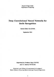
Table 1. Sample-level CNN configuration. For example, in the layer part, the first 3 of “conv 3-128” is the filter length, 128 is the number of filters, and 3 of “maxpool 3” is the pooling length. example of mn -DCNN models is shown in Table 1 where m is 3 and n is 9. According to the definition, the filter length and pooling length of the convolution layer are 3 other than the first strided convolution layer. If the hop size (stride length) of the first strided convolution layer is 3, the time-wise output dimension of the convolution layer becomes 19683 when the input of the network is 59049 samples. We call this “39 model with 19683 frames and 59049 samples as input”. 4. EXPERIMENTAL SETUP In the section, we introduce the datasets used in our experiments and describe detailed experimental settings. 4.1 Datasets We evaluate the proposed model on two datasets, Magnatagatune dataset (MTT) [16] and Million song dataset (MSD) annotated with the Last.FM tags [17]. We primarily examined the proposed model on MTT and then veri-

2n models model with 16384 samples (743 ms) as input

model with 32768 samples (1486 ms) as input

model

n

layer

filter length & stride

AUC

model

n

layer

filter length & stride

AUC

64 frames 128 frames 256 frames 512 frames 1024 frames 2048 frames 4096 frames 8192 frames

6 7 8 9 10 11 12 13

1+6+1 1+7+1 1+8+1 1+9+1 1+10+1 1+11+1 1+12+1 1+13+1

256 128 64 32 16 8 4 2

0.8839 0.8899 0.8968 0.8994 0.9011 0.9031 0.9036 0.9032

128 frames 256 frames 512 frames 1024 frames 2048 frames 4096 frames 8192 frames 16384 frames

7 8 9 10 11 12 13 14

1+7+1 1+8+1 1+9+1 1+10+1 1+11+1 1+12+1 1+13+1 1+14+1

256 128 64 32 16 8 4 2

0.8834 0.8872 0.8980 0.8988 0.9017 0.9031 0.9039 0.9040

3n models model with 19683 samples (893 ms) as input

model with 59049 samples (2678 ms) as input

model

n

layer

filter length & stride

AUC

model

n

layer

filter length & stride

AUC

27 frames 81 frames 243 frames 729 frames 2187 frames 6561 frames

3 4 5 6 7 8

1+3+1 1+4+1 1+5+1 1+6+1 1+7+1 1+8+1

729 243 81 27 9 3

0.8655 0.8753 0.8961 0.9012 0.9033 0.9039

81 frames 243 frames 729 frames 2187 frames 6561 frames 19683 frames

4 5 6 7 8 9

1+4+1 1+5+1 1+6+1 1+7+1 1+8+1 1+9+1

729 243 81 27 9 3

0.8655 0.8823 0.8936 0.9002 0.9030 0.9055

4n models model with 16384 samples (743 ms) as input

model with 65536 samples (2972 ms) as input

model

n

layer

filter length & stride

AUC

model

n

layer

filter length & stride

AUC

64 frames 256 frames 1024 frames 4096 frames

3 4 5 6

1+3+1 1+4+1 1+5+1 1+6+1

256 64 16 4

0.8828 0.8968 0.9010 0.9021

256 frames 1024 frames 4096 frames 16384 frames

4 5 6 7

1+4+1 1+5+1 1+6+1 1+7+1

256 64 16 4

0.8813 0.8950 0.9001 0.9026

5n models model with 15625 samples (709 ms) as input

model with 78125 samples (3543 ms) as input

model

n

layer

filter length & stride

AUC

model

n

layer

filter length & stride

AUC

125 frames 625 frames 3125 frames

3 4 5

1+3+1 1+4+1 1+5+1

125 25 5

0.8901 0.9005 0.9024

625 frames 3125 frames 15625 frames

4 5 6

1+4+1 1+5+1 1+6+1

125 25 5

0.8870 0.9004 0.9041

Table 2. Comparison of various mn -DCNN models with different input sizes. m refers to the filter length and pooling length of intermediate convolution layer module, and n refers to the number of the modules. Also, filter length & stride indicates the value of the first convolution layer. In the layer part, the first 1 of 1+n+1 is the strided convolution layer, and the last 1 is convolution layer which works like fully connected layer. fied the effectiveness of our model on MSD which is much larger than MTT (MTT contains 170 hours long audio, and MSD contains 1955 hours long audio in total). We filtered out the tags and used most frequently labeled 50 tags in both datasets, following the previous work [11], [14, 15] 1 . Also, all songs in the two datasets were trimmed to 29.1 second long. We used AUC (Area Under Receiver Operating Characteristic) as a primary evaluation metric for music auto-tagging.

1 https://github.com/keunwoochoi/MSD_split_for_ tagging

4.2 Optimization We trained the networks with the following settings: binary cross entropy loss with sigmoid activation on prediction layer is set to objectives. Batch normalization [18] and ReLU activation for every convolution layer is used. We should note that, in our experiments, batch normalization plays a vital role in raw waveform based deep learning. Dropout of 0.5 was applied to the output of the last convolution layer. We trained the models using stochastic gradient descent with 0.9 Nesterov momentum. The learning rate was initially set to 0.01 and decreased to a factor of 5 when the validation loss did not decrease more than 3 epochs. A total decrease of 4 times, the learning rate of the last training was 0.000016. Also, we used

3n models, 59049 samples as input

n

window (filter length)

hop (stride)

AUC

Frame-level (mel-spectrogram)

4 5 5 6 6

729 729 243 243 81

729 243 243 81 81

0.9000 0.9005 0.9047 0.9059 0.9025

Frame-level (raw waveforms)

4 5 5 6 6

729 729 243 243 81

729 243 243 81 81

0.8655 0.8742 0.8823 0.8906 0.8936

Sample-level (raw waveforms)

7 8 9

27 9 3

27 9 3

0.9002 0.9030 0.9055

Table 3. Comparison of three CNN-based models with different window (filter length) and hop (stride) sizes. n represents the number of intermediate convolution and maxpooling layer modules, thus 3n times hop (stride) size of each model is equal to the number of input samples. input type

model

MTT

MSD

Frame-level (mel-spectrogram)

Persistent CNN [19] 2D CNN [14] CRNN [15]

0.9013 0.894 -

0.851 0.862

This work

0.9059

-

Frame-level (raw waveforms)

1D CNN [11]

0.8487

-

Sample-level (raw waveforms)

This work

0.9055

0.8812

Table 4. Comparison of our works to prior state-of-the-arts batch size of 23 for MTT and 50 for MSD, respectively. In mel-spectrogram based model, we conducted the input normalization simply by dividing standard deviation after subtracting mean value of entire input data. On the other hand, we did not perform the input normalization on raw waveform based model. 5. RESULTS In this section, we examine proposed methods and finally compare them to previous state-of-the-art results. 5.1 mn -DCNN models Table 2 shows the evaluation results for the mn -DCNN models on MTT for different input sizes, number of layers, filter length and stride of the first convolution layer. As described in Section 3.4, m refers to the filter length and pooling length of intermediate convolution layer module, and n refers to the number of the modules. In Table 2, we can first find that the accuracy is proportional to n in most m. Increasing n in our model with the same m

value and input size means that the filter length and stride of the first convolution layer go down to sample-level (e.g. 2 or 3 size). When the first layer’s filter length and pooling length reach the sample-level, the sample-level architectures are simply seen as models constructed with the same filter length and sub-sampling length in all convolution layers as depicted in Table 1. The best results were obtained when m was 3 and n was 9. Interestingly, the length of 3 corresponds to the 3-size spatial filters in the VGG net [2]. In addition, we can see that 1-3 seconds of audio as input length to the network is also a reasonable choice in raw waveform based model as in mel-spectrogram based model. As a result, we find that deep models (more than 10 layers) with 1-3s audio as input having a very small sample-level filter length and sub-sampling length is very effective at learning raw waveforms in the music auto-tagging task. 5.2 Mel-spectrogram and raw waveforms Based on the fact that the output size of the first convolution layer of the model that uses the raw waveform is equivalent to the mel-spectrogram size that shares filter length (window), stride (hop) and the number of filters (the number of mel-bands), we further validate the effectiveness of the proposed sample-level architecture by performing experiments presented in Table 3. The models used in the experiments follows our model configuration strategy described in Section 3.4. We added a convolution layer and a pooling layer module at the top module of the 3n−1 model to compress all time dimensions to 1 in the 3n model. In the mel-spectrogram experiments, 128 mel-bands are used to match the number of filters of first convolution layer of raw waveform based model. FFT size was set to 729 in all comparisons and magnitude compression is applied with a nonlinear curve, log(1+C|A|) where A is the magnitude and C is set to 10. The results in Table 3 show that sample-level raw waveform based model achieves results comparable to the framelevel mel-spectrogram based model. We also found that using a smaller hop size (4 ms) than conventional approaches using hop size of 20 ms or so increased the performances significantly. However, if the hop size is less than 4 ms, the performance degrades. An interesting finding from the result of frame-level raw waveform based model is that when the filter length is larger than the stride, the accuracy was slightly lower than the models sharing filter length and stride. We interpret that this phenomenon is due to the learning ability of phase variances. As the filter length decreases, the extent that phase variance that the filter should learn is reduced. 5.3 MSD result and the number of filters We investigate the capacity of our sample-level architecture even further by evaluating the performance on MSD that is ten times larger than MTT. The result is shown in Table 4. While training the network on MSD, the number of filters in the convolution layers have been shown to affect performance. According to our preliminary test results, increasing the number of filters from 16 to 512 along

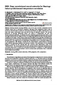
Layer 1

Layer 2

Layer 3

Layer 4

Layer 5

Layer 6

Figure 2. Spectrum of the filters in the sample-level convolution layers which are sorted by magnitude of frequency band. The x-axis represents the index of the filter, and the y-axis represents the frequency. The model used for visualization is 39 -DCNN with 59049 samples as input. Visualization was performed using the gradient ascent method to obtain the input waveforms that maximizes each filter in the layers. Based on the advantage of our model consisting solely of the convolution layer, we visualized the learned filter characteristics more distinctly, by back-propagating random noise of 729 samples as input. the layers was sufficient for MTT. However, the test on MSD shows that increasing the number of filters in the first convolution layer improves the performance. Therefore, we increased the number of filters in the first convolution layer from 16 to 128. 5.4 Comparison to state-of-the-arts In Table 4, we show the performance of the proposed architecture to previous state-of-the-arts on MTT and MSD. They show that our proposed sample-level architecture is highly effective compared to them. 5.5 Visualization of learned filters The technique of visualizing the filters learned at each layer allows better understanding of representation learning in the hierarchical network. However, previous works in music domain are limited to visualizing learned filters only on the first convolution layer [11, 12]. Especially the gradient ascent method has been proposed [20] for filter visualization and this technology has provided deeper understanding of what convolutional neural networks learn from images [21, 22]. Thus, we applied the gradient ascent method to see how each layer of the proposed network hears the raw waveforms. The gradient ascent method is as follows. First, we generate random noise and back-propagate to the trained network. The loss is set to the target filter. Then, we add the bottom gradients to the input with gradient normalization. By repeating this process several times, we can obtain the waveforms that maximizes the target filter at the input. With the advantage that any dimension can be an input as long as it meets the sub-sampling dimension of the convolution layer because our sample-level DCNN consists solely of a single convolution layer, we could visualize the sorted spectrum in Figure 2 or the learned filters in Figure 3 more clearly using noise of 729 samples as input. The layer 1 shows the three distinctive filter bands which is possible with the filter length with 3 samples. The center frequency of the filter banks increases linearly in low fre-

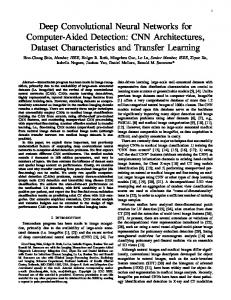
Figure 3. Examples of learned filters at each layer.

quency filter banks but it becomes non-linearly steeper in high frequency filter banks. This trend becomes stronger as the layer goes up. This nonlinearity was found in learned filters with a frame-level end-to-end learning [11] and also in perceptual pitch scales such as mel or bark. 6. CONCLUSION AND FUTURE WORK In this paper, we proposed sample-level DCNN models that take raw waveforms as input. Through our experiments, we showed that the deep architectures can improve the performance in music auto-tagging and they provide results that are comparable to previous state-of-the-art performances for the two datasets using raw waveforms as input. We also effectively visualized hierarchically learned filters. Future studies will analyze the learned filters more thoroughly by applying several visualization techniques. Furthermore, we can explore music style transfer at music or instrument level.

7. REFERENCES [1] A. Krizhevsky, I. Sutskever, and G. E. Hinton, “Imagenet classification with deep convolutional neural networks,” in Advances in neural information processing systems, 2012, pp. 1097–1105. [2] K. Simonyan and A. Zisserman, “Very deep convolutional networks for large-scale image recognition,” arXiv preprint arXiv:1409.1556, 2014. [3] T. Mikolov, I. Sutskever, K. Chen, G. S. Corrado, and J. Dean, “Distributed representations of words and phrases and their compositionality,” in Advances in neural information processing systems, 2013, pp. 3111–3119. [4] X. Zhang, J. Zhao, and Y. LeCun, “Character-level convolutional networks for text classification,” in Advances in neural information processing systems, 2015, pp. 649–657. [5] Y. Kim, Y. Jernite, D. Sontag, and A. M. Rush, “Character-aware neural language models,” arXiv preprint arXiv:1508.06615, 2015. [6] D. Palaz, M. M. Doss, and R. Collobert, “Convolutional neural networks-based continuous speech recognition using raw speech signal,” in Acoustics, Speech and Signal Processing (ICASSP), 2015 IEEE International Conference on. IEEE, 2015, pp. 4295–4299. [7] D. Palaz, R. Collobert et al., “Analysis of cnn-based speech recognition system using raw speech as input,” Idiap, Tech. Rep., 2015. [8] R. Collobert, C. Puhrsch, and G. Synnaeve, “Wav2letter: an end-to-end convnet-based speech recognition system,” arXiv preprint arXiv:1609.03193, 2016. [9] A. van den Oord, S. Dieleman, H. Zen, K. Simonyan, O. Vinyals, A. Graves, N. Kalchbrenner, A. Senior, and K. Kavukcuoglu, “Wavenet: A generative model for raw audio,” CoRR abs/1609.03499, 2016. [10] T. N. Sainath, R. J. Weiss, A. W. Senior, K. W. Wilson, and O. Vinyals, “Learning the speech front-end with raw waveform cldnns.” in INTERSPEECH, 2015, pp. 1–5. [11] S. Dieleman and B. Schrauwen, “End-to-end learning for music audio,” in Acoustics, Speech and Signal Processing (ICASSP), 2014 IEEE International Conference on. IEEE, 2014, pp. 6964–6968. [12] D. Ardila, C. Resnick, A. Roberts, and D. Eck, “Audio deepdream: Optimizing raw audio with convolutional networks.” [13] J. Pons, T. Lidy, and X. Serra, “Experimenting with musically motivated convolutional neural networks,” in Content-Based Multimedia Indexing (CBMI), 2016 14th International Workshop on. IEEE, 2016, pp. 1– 6.

[14] K. Choi, G. Fazekas, and M. Sandler, “Automatic tagging using deep convolutional neural networks,” in Proceedings of the 17th International Conference on Music Information Retrieval (ISMIR), 2016, pp. 805– 811. [15] K. Choi, G. Fazekas, M. Sandler, and K. Cho, “Convolutional recurrent neural networks for music classification,” arXiv preprint arXiv:1609.04243, 2016. [16] E. Law, K. West, M. I. Mandel, M. Bay, and J. S. Downie, “Evaluation of algorithms using games: The case of music tagging,” in ISMIR, 2009, pp. 387–392. [17] T. Bertin-Mahieux, D. P. Ellis, B. Whitman, and P. Lamere, “The million song dataset,” in Proceedings of the 12th International Conference on Music Information Retrieval (ISMIR), vol. 2, no. 9, 2011, pp. 591– 596. [18] S. Ioffe and C. Szegedy, “Batch normalization: Accelerating deep network training by reducing internal covariate shift,” arXiv preprint arXiv:1502.03167, 2015. [19] J.-Y. Liu, S.-K. Jeng, and Y.-H. Yang, “Applying topological persistence in convolutional neural network for music audio signals,” arXiv preprint arXiv:1608.07373, 2016. [20] D. Erhan, Y. Bengio, A. Courville, and P. Vincent, “Visualizing higher-layer features of a deep network,” University of Montreal, vol. 1341, p. 3, 2009. [21] M. D. Zeiler and R. Fergus, “Visualizing and understanding convolutional networks,” in European conference on computer vision. Springer, 2014, pp. 818– 833. [22] A. Nguyen, J. Yosinski, and J. Clune, “Deep neural networks are easily fooled: High confidence predictions for unrecognizable images,” in Proceedings of the IEEE Conference on Computer Vision and Pattern Recognition, 2015, pp. 427–436.