Sample-level sound synthesis with recurrent neural networks and

Sample-level sound synthesis with recurrent neural networks and conceptors Chris Kiefer Corresp. 1

1

Experimental Music Technologies Lab, Department of Music, University of Sussex, Brighton, United Kingdom

Corresponding Author: Chris Kiefer Email address: [email protected]

Conceptors are a recent development in the field of reservoir computing; they can be used to influence the dynamics of recurrent neural networks (RNNs), enabling generation of arbitrary patterns based on training data. Conceptors allow interpolation and extrapolation between patterns, and also provide a system of boolean logic for combining patterns together. Generation and manipulation of arbitrary patterns using conceptors has significant potential as a sound synthesis method for applications in computer music and procedural audio but has yet to be explored. Two novel methods of sound synthesis based on conceptors are introduced. Conceptular Synthesis is based on granular synthesis; sets of conceptors are trained to recall varying patterns from a single RNN, then a runtime mechanism switches between them, generating short patterns which are recombined into a longer sound. Conceptillators are trainable, pitch-controlled oscillators for harmonically rich waveforms, commonly used in a variety of sound synthesis applications. Both systems can exploit conceptor pattern morphing, boolean logic and manipulation of RNN dynamics, enabling new creative sonic possibilities. Experiments reveal how RNN runtime parameters can be used for pitch-independent timestretching and for precise frequency control of cyclic waveforms. They show how these techniques can create highly malleable sound synthesis models, trainable using short sound samples. Limitations are revealed with regards to reproduction quality, and pragmatic limitations are also shown, where exponential rises in computation and memory requirements preclude the use of these models for training with longer sound samples. The techniques presented here represent an initial exploration of the sound synthesis potential of conceptors; future possibilities and research questions are outlined, including possibilities in generative sound.

PeerJ Preprints | https://doi.org/10.7287/peerj.preprints.27361v1 | CC BY 4.0 Open Access | rec: 19 Nov 2018, publ: 19 Nov 2018

1

2

Sample-level sound synthesis with recurrent neural networks and conceptors

3

Chris Kiefer1

4

1 Experimental

5

Music Technologies Lab, Department of Music, University of Sussex, Brighton, UK. BN1 9RG

7

Corresponding author: Chris Kiefer1

8

Email address: [email protected]

9

ABSTRACT

6

10 11 12 13 14 15 16 17 18 19 20 21 22 23 24 25 26 27 28 29 30

31

32 33 34 35 36 37 38 39 40 41 42 43 44 45 46

Conceptors are a recent development in the field of reservoir computing; they can be used to influence the dynamics of recurrent neural networks (RNNs), enabling generation of arbitrary patterns based on training data. Conceptors allow interpolation and extrapolation between patterns, and also provide a system of boolean logic for combining patterns together. Generation and manipulation of arbitrary patterns using conceptors has significant potential as a sound synthesis method for applications in computer music and procedural audio but has yet to be explored. Two novel methods of sound synthesis based on conceptors are introduced. Conceptular Synthesis is based on granular synthesis; sets of conceptors are trained to recall varying patterns from a single RNN, then a runtime mechanism switches between them, generating short patterns which are recombined into a longer sound. Conceptillators are trainable, pitch-controlled oscillators for harmonically rich waveforms, commonly used in a variety of sound synthesis applications. Both systems can exploit conceptor pattern morphing, boolean logic and manipulation of RNN dynamics, enabling new creative sonic possibilities. Experiments reveal how RNN runtime parameters can be used for pitch-independent timestretching and for precise frequency control of cyclic waveforms. They show how these techniques can create highly malleable sound synthesis models, trainable using short sound samples. Limitations are revealed with regards to reproduction quality, and pragmatic limitations are also shown, where exponential rises in computation and memory requirements preclude the use of these models for training with longer sound samples. The techniques presented here represent an initial exploration of the sound synthesis potential of conceptors; future possibilities and research questions are outlined, including possibilities in generative sound.

INTRODUCTION Machine Learning and Sound Synthesis Current intersections between sound synthesis and machine learning are evolving quickly. We have seen significant progress in symbolic note generation (e.g. RL Tuner (Jaques et al., 2016), Flow Machines (Ghedini et al., 2016)), parametric control of sound synthesis models (e.g Wekinator (Fiebrink, 2011), automatic VST programming (Yee-King et al., 2018)) and also with current state of the art raw audio generation techniques. These recent advances in raw audio synthesis principally use deep architectures, for example WaveNet (Oord et al., 2016), SampleRNN (Mehri et al., 2016), NSynth (Engel et al., 2017) and WaveGAN (Donahue et al., 2018), to generate low-level audio representations (sample or spectral level) without using a synthesis engine, working as self-contained models that merge sound generation and control into one. There is also significant interest from the computer music community in sound synthesis with dynamical and chaotic systems, with strong connections to RNN techniques being used in contemporary deep architectures. This goes back to the earlier work of composers such as Roland Kayn who composed with electronic cybernetic systems, and is reflected in more recent work from, for example, Sanfilippo and Valle (2013) on feedback systems, Ianigro and Bown (2018) on sound synthesis with continuous-time


47 48 49 50

recurrent neural networks, Wyse (2018) on sound synthesis with RNNs and Mudd (2017) on nonlinear dynamical processes in musical tools. The work presented here draws on overlapping research in both machine learning and dynamical systems techniques, in the context of sound synthesis.

63

Reservoir Computing While many contemporary developments in machine learning and sound synthesis are based on deep neural network paradigms, pioneering work has also been taking place within the bio-inspired field of reservoir computing (RC) (Schrauwen et al., 2007). Within the RC paradigm, computation is performed using a structure that groups an untrained reservoir with a fixed input layer and a trainable output layer. The reservoir is a complex dynamical system which is perturbed by input signals and transforms these signals into a high-dimensional state space, the current state being dependent on both the current input and on a fading history of previous inputs. The output layer performs a linear transformation of the current reservoir state, and can be trained using supervised methods. RC systems can learn nonlinear and temporal mappings between the input and output signals. A reservoir can be created using both physical systems (e.g bacteria (Jones et al., 2007), a bucket of water (Fernando and Sojakka, 2003) or optics (Duport et al., 2016)) and digital systems. The latter usually take the form of liquid-state machines (Maass et al., 2002) or echo state networks (ESNs) (Jaeger, 2001).

64

Echo State Networks

51 52 53 54 55 56 57 58 59 60 61 62

65 66 67 68

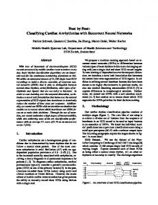
ESNs have so far been the primary technique employed for sound and music applications within the RC field. An ESN (see figure 1) uses a randomly generated recurrent neural network (RNN) as a reservoir. This reservoir is connected to inputs and output via single layers of weights. The output layer weights can be trained using linear optimisation algorithms such as ridge regression (Lukoˇseviˇcius, 2012, p. 10).

Figure 1. An example of an Echo State Network with ten sparsely connected nodes, single inputs and outputs, and fully connected input and output layers 69 70 71 72 73 74 75 76 77 78 79 80 81

ESNs are inherently suited to audio applications due to their temporal dynamics. Jaeger’s original work with ESNs included examples of models being trained to output discrete-periodic sequences and learning to behave as sine wave oscillators (Jaeger, 2001). Subsequently, ESNs have been applied to a range of creative sound and music tasks. These include symbolic sound generation tasks such as melody generation (Jaeger and Eck, 2006) and generative human-feel drumming (Tidemann and Demiris, 2008); direct audio manipulation and synthesis applications bear examples of amplifier modelling, audio prediction and polyphonic transcription (Holzmann, 2009b,a; Keuninckx et al., 2017); they have also been used for modelling complex mappings in interactive music systems (Kiefer, 2014). Under the classical ESN approach, as applied to the task of sound synthesis, ESNs are trained as audio rate pattern generators. A limitation of the classical ESN approach is that it is challenging to learn multiple attractors, corresponding to the generation of multiple patterns on different timescales with a single reservoir (Holzmann, 2009a). Holzmann proposed an extension to the ESN paradigm that helps to overcome these limitations by using specialised IIR filter neurons; these neurons tune areas of the 2/24


86

reservoir to different frequencies, therefore decoupling sections of the reservoir and allowing multiple attractors to form. Results showed that filter neurons enabled an ESN to learn to reproduce waveforms built additively from inharmonic sine waves, a task that was not achievable with a standard ESN. A recent development of the ESN paradigm comes in the form of conceptors, an addition to the basic architecture of ESNs that allow the behaviour of the reservoir to be controlled.

87

Conceptors

82 83 84 85

88 89 90 91 92 93 94 95 96 97 98 99 100 101

Conceptors (Jaeger, 2014a), offer a highly flexible method for generating and manipulating multiple patterns within single reservoirs. Conceptors are a mechanism for performing a variety of neurocomputational functions, the ones most relevant to sound synthesis being incremental learning and generation of patterns, morphing and extrapolation of patterns, cued pattern recall, and the use of boolean logic to combine patterns (Jaeger, 2014a). They work by learning the subset of state space visited by an RNN when driven by a particular input. They can then be used to restrict the RNN to operate with this subspace, functioning like an attractor (Gast et al., 2017). The separation of an RNN’s state space in this manner allows multiple attractors to be learned using the same network, and for combinations of these subspaces to be used to manipulate the dynamics and output of the RNN. The potential for combination of conceptors is a very powerful feature of this technique, and Jaeger describes boolean logic rules for achieving this (Jaeger, 2014b, p.50). Their strong potential for pattern generation, extrapolation and manipulation, and the combination of continuous and discrete-boolean methods of manipulation are compelling reasons to believe they will have strong applications in the field of audio and creative sound production.

116

New Sound Synthesis Methods Two new methods of conceptor-based sound synthesis are demonstrated. The first is conceptular synthesis. This is a synthesis method based on granular synthesis. Granular synthesis (Roads, 2004) is based on the sequencing, combination and manipulation of short (typically 20ms - 100ms) windowed segments (grains) of sampled sound. It is a powerful technique for creating and coherently manipulating sound; applications include time and pitch independent stretching of pre-recorded audio. In conceptular synthesis, an RNN model is trained to generate grains, which are recalled by conceptors. The second mode of synthesis is the conceptillator. This mode is based on the natural ability of conceptors to recall and manipulate cyclic waveforms, in order to learn RNN models of harmonically-rich oscillators; it explores further methods for sonic manipulation of these oscillators within the conceptor paradigm. In both of these methods, the use of conceptor based RNN models allows flexible sound manipulation through creative combinations of conceptors to influence reservoir behaviour. These two methods are described below. To begin with a mathematical description of the RNN and conceptor models common to both synthesis models is presented. This is followed by discussion of methodology, and accounts of the experiments that were carried out to develop these methods.

117

BASIC MODELS

102 103 104 105 106 107 108 109 110 111 112 113 114 115

118 119 120 121

122 123

This section summarises the fundamental methods used in the creation of the sound synthesis models described below. For a more detailed explanation of these methods, please refer to Jaeger’s extensive technical report on conceptors (Jaeger, 2014b). The basic model is an RNN consisting of N nodes, updated according to equations (1) - (3): xtarget (n + 1) = W x(n) +W in a(n + 1)

(1)

x(n + 1) = ((1 − α)xtarget (n)) + (αtanh(xtarget (n + 1) + b))

(2)

y(n + 1) = W out x(n + 1)

(3)

At discrete time step n, activation levels for each RNN node are stored in state vector x(n) of size N. The nodes are sparsely connected with a probability of 10.0/N in weight matrix W (of size N x N). An 3/24


124 125 126 127 128 129 130 131 132 133 134 135 136 137

138 139 140 141 142 143 144 145 146 147 148 149 150 151 152

153

154 155 156 157 158

input signal vector a(n) (size 1) is fully connected to the neurons with the input weight matrix W in (size N x 1). W in is generated using linear random values between −1 and 1, and scaled using input scaling factor γ input . Reservoir weight values are randomly chosen from a normal distribution, scaled according to the spectral radius γ W (to limit the maximum absolute eigenvalue), and then optimised during training. b is a vector of N biases, which are generated from a linear random distribution between −1 and 1, and scaled with bias scaling factor γ bias . Output weights W out are a matrix of size 1 x N, whose values are optimised during training. The output vector y(n) is a vector of size 1. The tanh smoothing function ensures that the reservoir states remain in the range −1 to 1, and introduces a nonlinearity into each node. α is a leaky integration coefficient (Lukoˇseviˇcius, 2012). This adds a one-pole lowpass filter to each node; lowering α (between 0 and 1) will slow down reservoir dynamics. This parameter can be fine-tuned to align the temporal dynamics of the reservoir to those of the desired output. A model is trained in two phases: (a) audio signals a j (n) are loaded into the model (see below), so that they can later be reproduced, (b) a conceptor is calculated for each audio signal. Following training, the model and conceptors are combined and manipulated to synthesise sound. Loading Patterns into the Model In this phase of training, a set of reservoir weights W ∗ are adapted so that the model can reproduce a set of driving audio signals a, resulting in a new set of weights W . W is optimised such that (a) W x j (n) ≈ W ∗ x j (n) +W in a j (n), i.e. the reservoir can simulate the driving inputs in their absence, and (b) the magnitudes of weights W are minimised. The process works as follows: for each pattern a j (n), the reservoir with weights W ∗ is driven from an initial randomised state for Lwashout + Ltrain steps using equations 1 and 2, and the resultant reservoir states are collected. The states x(n) from timesteps Lwashout − 1 . . . Lwashout + Ltrain − 1 are stored in N x Ltrain matrix, Xe j ; states x(n) from timesteps Lwashout . . . Lwashout + Ltrain are stored in N x Ltrain matrix, X j ; states xtarget (n) from timesteps Lwashout . . . Lwashout + Ltrain are stored in N x Ltrain matrix, M j . The remaining timesteps are discarded, to remove the effects of the initial state on reservoir dynamics. The driving signals from steps from timesteps Lwashout . . . Lwashout + Ltrain are stored in 1 x Ltrain matrices P j . These collections are concatenated into matrices Xe = [Xe1 |Xe2 | . . . Xen ], X = [X 1 |X 2 | . . . X n ], M = 1 [M |M 2 | . . . M n ] and P = [P1 |P2 | . . . Pn ] W and W out can now be calculated using ridge regression: e ′ )′ W = ((XeXe′ + ρ W INxN )−1 XM

(4)

W out = ((XX ′ + ρ out INxN )−1 XP′ )′

(5)

In both of the above, I is an identity matrix and ρ W and ρ out are regularisation factors. Calculating Conceptors Conceptors can take several forms, the form used in this study is the alloconceptor (Jaeger, 2017, p18), a matrix conceptor that is calculated after patterns are loaded into the network, and inserted into the update loop of the network at runtime. To calculate a conceptor which will influence the RNN to reproduce audio signal a j (n), the reservoir state correlation matrix R is initially calculated:

R= 159

X j (X j )′ Ltrain

The singular value decomposition (SVD) of R is found U j S j (U j )′ = R j

160

(6)

(7)

S j is modified, and then used to calculate the conceptor C j : Snew = S j (S j + α −2 INxN )−1

(8) 4/24


C j = U j Snew (U j )′ 161 162 163

164 165

(9)

α is the aperture of the conceptor (Jaeger, 2014b, p35). The optimal value for α can be found programatically (see below). The new conceptor can now be inserted to the runtime loop of the RNN: z(n + 1) = tanh(W x(n) + b)

(10)

x(n + 1) = C j z(n + 1)

(11)

An optimal value for α corresponds to the minimum value of attenuation aC,α (Jaeger, 2014b, p47), which can be calculated as follows:

aC,α =

E[||z(n) − x(n)||2 ] E[||z(n)||2 ]

(12)

170

when the network is updated using equations 10 and 11. The result of this training process is an RNN coupled with a set of conceptors; this model is referred to as a conceptor-controlled recurrent neural network (CCRNN). These basic methods are used in all the experiments below, and expanded on with new techniques that allow training and exploitation of the models for sounds synthesis.

171

METHOD AND MATERIALS

166 167 168 169

172 173 174 175 176 177 178 179 180 181 182 183 184 185 186 187 188 189 190 191 192 193 194

195 196 197 198 199 200

This project asks how the pattern generation ability of CCRNNs can be applied to field of sound synthesis. It aims to establish and evaluate the fundamental capabilities of CCRNNs to be trained to reproduce arbitrary audio signals, and to explore their creative affordances. Five experiments are presented, grouped into two categories; experiments 1 - 3 evaluate the potential of CCRRNs to resynthesise sampled sounds of increasing complexity, experiments 4 and 5 evaluate the use of CCRNNs as pitched oscillators for harmonically rich waveforms. In both categories, the ability of trained models to reconstruct the training signal is used as a measure of basic success in sound synthesis. Reconstruction ability is the core indication of sound synthesis quality, although this evaluation only tells part of the story, as the techniques outlined in this project are intended for open-ended use in creative sound synthesis applications. To this end, the project maps out key methods for parameterising and manipulating CCRNN sound synthesis models to create new sonic variations of the original training material. Both experiments establish the technical strengths and limitations of CCRNN sound synthesis, and identify open questions for future research in this area. In the experiments described below, there is some discussion of processing time to indicate the scale of computation involved with these techniques. The conceptular synthesis experiment was run on a laptop with a 2.5 GHz i7 CPU. The conceptillator experiments were run on an NVidia GTX 1080 Ti GPU using TensorFlow. Supplemental sound examples and figures are available at https://doi.org/10.25377/ sussex.7321826. Python 3 source code in Jupyter notebooks for all experiments is provided at https://github.com/chriskiefer/conceptorSoundSynthesis. A working implementation of conceptular synthesis in the form of a drum synthesiser can be found at https://conceptular.luuma.net/ with source code at https://github.com/ chriskiefer/conceptularBeatSynth. Error and Similarity Following from wider literature in reservoir computing, this project uses Normalised Root-Mean-Square Error (Lukoˇseviˇcius, 2012, p2) (NRMSE) to measure similarity between time series; lower values indicating higher similarity. NRMSE does not reflect perceptual aspects of sound similarity; these are crucial to understanding the results therefore, where relevant, spectrograms are displayed for visual comparison, and audio is included in the dataset accompanying this paper. 5/24


201 202 203 204 205 206 207 208 209 210 211 212 213 214 215 216 217 218 219 220 221 222 223 224

225 226 227 228 229 230 231 232

233 234 235

CONCEPTULAR SYNTHESIS Conceptular synthesis expands on an established method of sound synthesis, granular synthesis. The core concept behind granular synthesis is to break down a sound into small parts called grains, and then recombine these grains in different ways to produce new sounds. The theoretical roots of this method lie in Gabor’s (1947) theory of acoustic quanta, and in the compositional theory of Xenakis (1971). Digital implementations of the technique were developed by Roads (1978) and Truax (1986). Granular synthesis is a widely-used sound production method in contemporary electronic music, having been implemented in many established software systems. It offers methods for further sound manipulation techniques including timestretching (Truax, 1994) and corpus-based concatenative synthesis (Schwarz, 2006). The ability of CCRNNs to be trained to generate arbitrary sequences suggests that they could become powerful sound synthesis tools, as they can theoretically reproduce arbitrary waveforms. However they are pragmatically limited to playing relatively short sequences; the reason for this is that the computational complexity of the model increases exponentially with the number of nodes in the RNN, and the number of RNN nodes needed for regenerating a sequence increases with its length. However, if a model is trained to reproduce a set of shorter sound sequences, then granular synthesis techniques can be used to recombine these sequences to produce longer sounds. Conceptular synthesis therefore expands upon granular synthesis, by dynamically generating grains using conceptors rather than replaying grains from sound sample data. Grain patterns are loaded into an RNN, and conceptors force the RNN to replay specific grains. A granular synthesis-style control mechanism is used to switch conceptors so that the model generates a sequence of short patterns, which are combined into a longer waveform. Using dynamic models in this way instead of static patterns data the sonic potential of this synthesis method, as the model can be manipulated in addition to the recombination mechanism. Three experiments are described below, which resulted in the development of two variations of this synthesis technique. Experiment 1: Resynthesis of a Snare Drum The objective of this experiment was to subdivide an audio sample into a set of sub-sequences, and learn an RNN and set of conceptors that could regenerate these sub-sequences, with the intention of recreating the audio sample by recombining the model-generated sequences. A snare drum was chosen as a simple entry into exploring this new method of synthesis, using a short sound with a relatively simple envelope and harmonic structure. A method is presented below for resynthesising this sample using conceptors; this method was optimised by hand-tuning parameters. The key ways in which the method is parameterised are then discussed. Method

The sound (see figure 2 and Audio S1) was re-sampled at 22050 Hz (half of CD-quality), in order to reduce the CPU load of training, and to reduce the pattern length that the networks would need to learn.

Amplitude

0.8 0.6 0.4 0.2 0.0 −0.2 −0.4 −0.6 0

500

1000

1500

Time (samples)

2000

2500

3000

Figure 2. The waveform of the snare drum sample used to train the model in experiment 1. 236 237 238 239 240 241 242

The sample was then divided into a set of equal length signals a, of length µ samples each. A model was trained to reproduce the set of signals a using the methods described above. The model parameters are shown in table 1. The first 100 audio signals in set a were used to calculate a model (see figure 3). The RNN is initialised randomly, resulting in variance in the quality of reservoirs which is reflected in the NRMSE between (a) the target reservoir states and their approximation using the learned weight matrix W (nrmseW ) and (b) the target output states and their approximation calculated using the reservoir 6/24


Table 1. Model parameters for experiment 1. N

γW

γ input

γ bias

α

µ

Lwashout

Ltrain

ρW

ρ out

900

1.5

1.2

0.5

0.99

15

4µ

4µ

0.0001

0.001

Amplitude

0.8 0.6 0.4 0.2 0.0 −0.2 −0.4 −0.6 0

2

4

6

8

10

Time (samples)

12

14

Figure 3. The snare waveform was divided into 15-sample sequences, this diagram shows the first 50 of them

243 244 245 246 247 248 249

250 251 252 253

and output later W out (nrmsereadout ). When choosing a reservoir in the experiment, a brute-force search was used; 30 randomly generated reservoirs were trained, and the model with the lowest nrmsereadout of 0.008 was chosen. A conceptor C j was calculated for each signal a j . To reconstruct the sample from the model, the RNN was initially run for Lwashout steps with the first conceptor C0 . The model was then run with each conceptor C j inserted into the update loop, as described in equations 10 and 11, to create a set of output signals q, each of length µ. Finally, the signals were appended to create the waveform k = [q0 |q1 | . . . |qn ]. Results

The reconstruction error for each individual conceptor C j was measured, for generating signal a j . Supplemental figure S1 shows graphs of each result. The signals were reconstructed with a mean NRMSE of 0.73 (min: 0.174, max: 1.363, distribution shown in figure 5).

Amplitude

0.6 0.4 0.2 0.0 −0.2 −0.4 −0.6

0

200

400

600

800

Time (samples)

1000

1200

1400

Figure 4. The waveform of the reconstructed snare drum, produced using conceptular synthesis with the model trained in experiment 1. 254 255 256 257 258 259 260 261 262 263 264 265

Figure 4 shows the reconstructed sample, and figure 6 shows the reconstruction overlaid against the original. The sample can be heard in supplemental audio S2. The NRMSE error between these two samples was 1.15. In the rendering of the sample, the RNN activations x are initialised from a normal distribution. This causes subtle variations in each rendering; over 500 renderings, NRMSE errors varied between 1.148 and 1.163, with a mean of 1.156. Much of the variance occurred at the start of the renderings, within the first 400 samples. The variations tend to follow an approximately similar form, most likely due to the conceptor restricting the behaviour of the RNN within bounds. This points to the potential use of CCRNNs as generators of constrained random variations of sounds, which is explored later in the paper. The spectra of the original and reconstructed samples are shown in figure 7. It can be seen that the resynthesis produces an approximation of the original sample. In the time domain, the waveforms follow a similar envelope, although the reconstruction is missing some high frequency detail. The spectrograms 7/24


%

12 10 8 6 4 2 0

0.2

0.4

0.6

0.8

NRMSE

1.0

1.2

1.4

Amplitude

Figure 5. Distribution of NRMSE reconstruction errors for the individual audio signals used to train the model in experiment 1. 0.8 0.6 0.4 0.2 0.0 0.2 0.4 0.6

Reconstruction Original

0

200

400

600

800

Time (samples)

1000

1200

1400

Figure 6. A waveform comparison of the original snare sample, and the sample produced by the trained model.

266 267

268 269 270 271 272 273 274 275 276 277 278 279 280 281 282 283 284 285 286 287 288 289 290 291

292 293 294 295

show similar broad structure, although the reconstruction introduces artefacts, particularly in lower frequencies. Key Parameters

There are two key parameters that affect the reconstruction quality: the model size N and the length of the signals into which the sample is divided, µ. Predictably, as N increases, so does the quality of reconstruction. This is supported by the broader literature on echo state networks, showing that N correlates with the memory capacity of the network, and the N should be at least equal to the number of independent variables needed for the task the model is being trained for (Jaeger, 2002). In this case, as we increase the number and size of patterns, we need to increase N. The other key parameter is the signal length µ. An investigation was carried out into the relationship between these two parameters. Models were evaluated for all combinations of N ∈ {200, 400, 600, 800, 1000} and µ ∈ {5, 15, 25, 35, 45, 55, 65}. For each parameter combination, five models were trained and tested, and the number of signals was selected to total 1500 samples. Each model was scored on the average NMRSE error for reconstruction of each individual signal. Figure 8 shows the results, with the surface representing the average score for each parameter combination, and the red dots showing the actual scores. The graph demonstrates that the optimal value for µ was, in this case of this particular sample, 15, with reconstruction error decreasing with larger values of N. It also reveals a smooth error surface, showing that the optimal value for reproducing a particular sample could be determined by gradient based optimisation rather than brute force search. Decreasing µ brings practical constraints; µ is inversely proportional to the number of patterns that the network must be trained to reproduce. For each pattern, an individual conceptor is needed, and large numbers of conceptors can put pressure on memory resources. For example, the resynthesis of the snare sample in this experiment with µ = 15 and N = 900 results in 619 MB of conceptor data. A grain size of 15 samples is much smaller than in standard granular synthesis; at 22050Hz, 15 samples represents 0.68ms, whereas granular synthesisers might use grains from 20-100ms (although there is no fixed rule for this). Extended Sound Synthesis Parameters

The sound generation algorithm has three key parameters: speed, leak rate scale, and weight scaling. The speed parameter changes the amount of time in which the algorithm waits until a new conceptor is plugged in to the RNN update loop, therefore forcing it to generate a different pattern. For example, 8/24


Reconstruction +0 dB 8192 -10 dB 4096 -20 dB 2048

-30 dB

Hz

1024

-40 dB

512

-50 dB

256

-60 dB

128

64

-70 dB

0

-80 dB

Original +0 dB 8192 -10 dB 4096 -20 dB 2048

-30 dB

Hz

1024

512

256

128

-40 dB

-50 dB

-60 dB

64

-70 dB

0

-80 dB

Figure 7. A spectral comparison of the original snare sample, and the sample produced by the trained model.

Figure 8. A comparison of NRMSE reconstruction errors between the original snare sample and the output of trained models, while varying N and µ

9/24 PeerJ Preprints | https://doi.org/10.7287/peerj.preprints.27361v1 | CC BY 4.0 Open Access | rec: 19 Nov 2018, publ: 19 Nov 2018

296 297 298 299 300 301 302

a speed of 0.5 results in two cycles of a pattern being played for each conceptor C j and resulting in a rendered sample that is twice the length of the original. In the case of resynthesising this snare sample, a speed of 0.5 has the effect of pitching the sample down, and a speed of more than 1.0 pitches the sample up. At negative speeds, a sample can be crudely reversed by playing the patterns in reverse sequence. In the case of other models (see below), this parameter can have the effect of timestretching, i.e. extending or compressing the length of a sound, independent from its pitch. The leak rate α can be scaled during resynthesis, by updating equation 2 as follows: αscaled = α ∗ scaleα target

x(n + 1) = ((1 − αscaled )x 303 304 305 306 307 308 309 310 311

312 313 314 315 316 317 318 319

320 321 322 323

(13)

(n)) + (αscaled tanh(xtarget (n + 1) + b))

scaleα should be limited such that α stays between 0 and 1. In the case of this snare sample, reducing α removed high frequencies from the rendered samples. In other models (again, see below), changing α can have the effect of changing the pitch of the output. The weight scaling scaleW parameter is a multiplier for the RNN weight matrix W ; this causes tonal changes in the rendered sample whose characteristics are based on the random make up of the RNN. There is some consistency in this parameter in that when raised, more high frequency content tends to be introduced. At higher values, the RNN can behave in musically interesting non-linear ways. Below a lower limit (model dependent), the model tends towards silence. Further manipulations of sound can be achieved by manipulating conceptors. Extending Sound Synthesis with Conceptor Logic

The use of conceptor logic and conceptor manipulation is where this mode of sound synthesis significantly moves on from standard granular synthesis features, and brings its own unique possibilities. New conceptors can be meaningfully created using boolean logic rules; Jaeger (2014b, p.52) defines formulae for AND, OR and NOT operations. Boolean operations with conceptors can be used to logically control RNNs, with applications in classification and memory management. In the case of conceptular synthesis, logic operations provide a wide range of creative possibilities. Conceptors can be logically recombined to create new tonal variations. Two examples are now given: Example 1

Each conceptor in the snare model C j is combined with the next three conceptors to make a new set C2 , using the rule C2j = C j ∨C j+1 ∨C j+2 ∨C j+3 This results in a variant on the original snare sound shown in figure 9.

Amplitude

0.2 0.0 0.2 0.4 0

200

400

600

800

Time (samples)

1000

1200

1400

Figure 9. The waveform of a variant of the snare sample, produced using boolean logic C2j = C j ∨C j+1 ∨C j+2 ∨C j+3

324 325 326 327 328 329 330

Example 2

A new set of conceptors C3 is made by combining each conceptor in the set with a random choice of two other conceptors in the set C3j = C j ∨ Crandom1 ∨ Crandom2 . This is designed with the intention of keeping the main structure of the sample but introducing random variations. Figure 10 shows the resulting waveforms from 4 iterations of the process. In both these examples, the variations are subtle, and the renderings suffer from some artefacts, however this does point to generative possibilities that are worthy of further research. 10/24


Amplitude

0.3 0.2 0.1 0.0 0.1 0.2 0.3

0

200

400

600

800

Time (samples)

1000

1200

1400

Figure 10. Waveforms showing generative variants of the snare sample, using the boolean logic rule C3j = C j ∨Crandom1 ∨Crandom2 331 332 333 334 335 336 337 338 339

Sound Morphing with Interpolated Conceptors

Jaeger (2014b, p.42) demonstrated shape morphing between heterogeneous patterns using conceptors. This same technique can be applied within conceptular synthesis to morph between sounds. Morphing can be implemented by creating a linear combination of conceptors to interpolate between the two patterns the conceptors were trained to recreate. Equation 14 shows how this can be done with two conceptors, where µ is the morphing factor. Varying µ between 0 and 1 forces the RNN to create a morph between the patterns represented by the two conceptors. When 0 ≤ µ ≤1, the mix of conceptors will interpolate between patterns. However, when µ is outside of this range, the mix of conceptors will extrapolate between patterns. x(n + 1) = ((1 − µ)Ci + µC j )tanh(W x(n) + b)

340 341 342 343 344 345 346 347 348 349 350 351 352 353

354 355 356 357 358 359 360 361 362 363 364 365 366 367 368 369

(14)

The intention of morphing between sounds is to create a new mixture of sounds that retains the shared perceptual properties of the original sources (Slaney et al., 1996). Morphing was investigated with conceptular synthesis by training an RNN and conceptors to recreate patterns from two different samples: the snare sample already discussed, and a short bongo sample. An 800-node network was trained, with an average NRMSE of 0.7685 for recreation of 100 individual patterns (length 15) for each sample, resulting in two sets of conceptors, Csnare and Cbongo . Morphing was achieved by creating a new set of conceptors based on a linear mixture of the trained conceptors, for each pattern segment. The results demonstrate a morph between samples that is noticeably different from a linear mixture of the two samples. Supplemental figure S2 shows how the time-domain waveform result varies over an 11 point morph from µ = 0 to µ = 1, and the result can be heard in supplemental audio S3. For comparison, supplemental figure S3 and audio S4 show a linear mix between the same two samples. Boolean conceptor logic can also be used for sound morphing. For example, a set of conceptors j = CbongoSnare was created, with each element combining elements from the snare and the bongo CbongoSnare j j Cbongo ∨Csnare . A sample rendered with this conceptor set contains characteristics of both sounds.

Discussion

This first experiment demonstrates how CCRNNs can be used to resynthesise short samples by dividing the sample up into short signals and training a conceptor for the reproduction of each one. The trained model offers malleable sound synthesis possibilities when manipulated using inherent runtime parameters and through conceptor combinations created either by mixing or by boolean logic. The models created in the experiment could not perfectly reproduce the training samples, but were able to make recognisable reconstructions. There is a variability between models, due to random initialisation of the RNN. This variability is minimised when using the network within normal constraints, however when pushed into non-linear modes of behaviour by, for example, changing the value of scaleW , a higher variability between different CCRNNs can be observed. This behaviour for a particular network may turn out to be musically interesting, lending conceptular synthesis potential for serendipitous discovery of new sounds, and a level of generative unpredictability that is often valued by musicians (McCormack et al., 2009). Conceptor logic offers a system to create new conceptors that produce coherent variations of the sounds the model was trained to reproduce. These offer a powerful and open system for sound design. An audio synthesis process would ideally run in realtime so that musicians can interact with it through musical controllers and use it in musical performance. In this example, the rendering speed was around 11/24


370 371 372 373

374 375 376

Experiment 2: Resynthesis of a Kick Drum This experiment explored conceptular synthesis further, using a sample with different characteristics from the snare in experiment 1. A kick drum sample was used (see figure 11 and supplemental audio S5). It can be seen that the sample has an initial high frequency component, followed by oscillations that gradually decrease in frequency and amplitude.

Amplitude

377

28 times slower than realtime, using a modern CPU. While this is far behind realtime, it should be noted that this version was not optimised for speed, and a dedicated C++ or GPU renderer is expected to be faster than the python version used here. It does however show the scale of computation involved in this method of sound synthesis, and indicates that computational resources are a challenge in this area.

0.6 0.4 0.2 0.0 0.2 0.4 0.6 0.8

0

2000

4000

Time (samples)

6000

8000

Figure 11. The waveform of the kick drum sample used in experiment 2 378

379 380 381 382 383 384 385 386 387 388 389

Failure with constant µ

The first attempt at resynthesis used the same method as in experiment one, slicing the original sample into equal sized sections and training a conceptor for each of these sections. This method proved to be unsuccessful at resynthesising the kick drum. Attempts at hand tuning the slice length µ and leak rate α all resulted in unwanted distortion. Small values of µ resulted in training set of patterns that were much smaller than the wavelengths in the original sample, each containing small and very slowly varying values. The network failed to learn these low frequencies. A very slightly better approach was to use a large value of µ that could capture whole cycles of oscillation. Figure 12 shows an example result from this approach, with µ = 200 and α = 0.3 (see also supplemental audio S6). Some segments of the reconstruction are successful, however the quality degrades as the wavelength in the original sample increases and there are significant artefacts presents.

Amplitude

2 1 0 1 2 0

500

1000

1500

Time (samples)

2000

2500

3000

Figure 12. A comparison of the original kick drum sample and the results of resynthesis using a model trained with the methods established in experiment 1. This method produced many unwanted artefacts. 390 391

392 393 394

Given that this negative result was clearly caused by using a fixed size for segmenting the audio sample, a new method of pattern segmentation with variable lengths was investigated. Method

A detector was used to locate zero-crossing points in the kick drum sample, resulting in a set of points i at which the sample was sliced to create a set of driving audio signals a (see figure 13).

i = {n|y(n) > 0 ∧ y(n + 1) < 0}

(15) 12/24


395

This simple approach to segmentation worked well for this particular sample but may not generalise to samples with higher harmonic complexity.

Amplitude

396

0.6 0.4 0.2 0.0 0.2 0.4 0.6 0.8

0

100

200

300

Time (samples)

400

Figure 13. Driving audio signals from the kick drum sample, segmented at zero-crossing points instead of using a constant value of µ 397 398

This set of patterns was used to train a new model, with the parameters as shown in table 2, which were manually optimised. Table 2. Parameters used for training the model in experiment 2

399 400 401

402 403 404 405 406

γW

γ input

γ bias

α

Lwashout

Ltrain

ρW

ρ out

900

1.5

1

0.5

0.25

2µ

2µ

0.0001

0.0001

For playback, the conceptular synthesis algorithm was altered in two ways. Firstly, the facility was added to play back patterns of varying length. Secondly, the algorithm was modified to linearly crossfade between conceptors, over a percentage of the pattern length. Results

The trained model reconstructed individual driving audio signals with a mean NRMSE of 0.091 (see supplemental figure S4 for reconstruction plots of each pattern). The kick drum sample was resynthesised using the conceptular synthesis algorithm, with the crossfade length set at 5% of signal length. The result is shown in figures 14 and 15, and included in supplemental audio S7. Both show a close reconstruction of the original, with the addition of some small, high frequency artefacts.

Amplitude

407

N

0.6 0.4 0.2 0.0 0.2 0.4 0.6 0.8


0

2000

4000

Time (samples)

6000

8000

Figure 14. A comparison of the original kick drum sample and the output of the trained model in experiment 2. 408 409

410 411 412 413 414 415 416

The model responds well to the extended sound synthesis manipulations described earlier. Supplemental audio S8 presents an example of timestretching from 50% up to 800% in 50% steps. Analysis

The experiment began with a failure of constant pattern sizes, and found success by segmenting variable length patterns using a simple zero-crossing detection algorithm. The original methods of cutting patterns at points based on position but with arbitrary amplitudes introduced high-frequency artefacts that negatively impacted the training of the model. By removing these artefacts with segmentation at zero-crossing points, the model could be trained to reproduce patterns that matched its broader dynamics, which were slowed down with a low α value. The result delivered clean resynthesis of the original sample 13/24



-30 dB

Hz

1024

-40 dB

512

-50 dB

256

-60 dB

128

-70 dB

64

0

-80 dB

Original +0 dB 8192 -10 dB 4096 -20 dB 2048

-30 dB

Hz

1024

-40 dB

512

-50 dB

256

-60 dB

128

64

-70 dB

0

-80 dB

Figure 15. Spectrograms comparing the resynthesised kick drum to the original sample in experiment 2.

417 418 419

420 421 422 423 424

425 426 427 428 429

and reasonable quality timestretching. This new approach was needed because of the low-frequency characteristics of the source sample, and probably worked well due to the relatively simple structure of the waveform. The next experiment tests these approaches on a more complex sound. Experiment 3: Vocal Sound The first two experiments attempted to reproduce shorts sounds with fairly simple structures. This next experiment attempts a more challenging resynthesis, of the complexity of the human voice. The source sample is a recording of someone saying the word ‘two’ (supplemental audio S9, Heston (2013)). This was chosen as it has a complex spectral variation over a short time period. Method Phase 1

An initial approach was to repeat exactly the same settings from experiment two, and to slice the sample according to the same zero-crossing algorithm. The only difference was to use α = 0.92, which was an optimal value determined through manual experimentation. Segmentation resulted in 197 driving audio signals, and conceptors were calculated to reproduce each one.

433

Phase 2 To refine the initial approach, a subset of the source sample was resynthesised - the ‘oo’ sound of ‘two’, described by 70 driving audio signals. To increase the resynthesis quality, the model size was set to N = 1400. This was the maximum model size possible given the computing resources available. In both phases, sound were resynthesised with a 5% crossfade between conceptors.

434

Results

430 431

Amplitude

432

0.75 0.50 0.25 0.00 0.25 0.50 0.75 1.00


0

2000

4000

6000

Time (samples)

8000

10000

Figure 16. A comparison of waveforms: the original ’two’ sample and the resynthesised version from the model trained in experiment 3.



-30 dB

Hz

1024

-40 dB

512

-50 dB

256

-60 dB

128

-70 dB

64

0

-80 dB

Original +0 dB 8192 -10 dB 4096 -20 dB 2048

-30 dB

Hz

1024

-40 dB

512

-50 dB

256

-60 dB

128

64

-70 dB

0

-80 dB

Figure 17. Spectrograms comparing the resynthesised ’two’ to the original sample in phase 1 of experiment 3.

435 436 437 438 439

Amplitude

440

Figure 16 shows the resynthesis results in the time domain, and figure 17 shows the spectrograms. The mean NRMSE for reconstructed driving audio signals was 3.31. This phase of the experiment delivered a poor reconstruction. Subjectively, the word ‘two’ can be heard within the resulting sound (see supplemental audio S10), but it is significantly masked by artefacts and distortion. This is reflected in the spectra and waveforms, where it can be seen that some elements correspond, but there are also significant deviations from the original. Phase 1

0.4 0.3 0.2 0.1 0.0 0.1 0.2 0.3 0.4


0

1000

2000

Time (samples)

3000

4000

Figure 18. Waveform comparison of the reconstructed ’oo’ and the original ’oo’, in phase 2 of experiment 3. 441 442 443

444 445 446 447 448 449 450 451 452 453 454

The time domain and spectral comparisons are shown in figures 18 and 19. The driving audio signals were reconstructed with an average NRMSE of 0.3. The resynthesis (Supplemental Audio S11), subjectively, sounds close to the original, with a NRMSE of 1.38. Phase 2

Discussion

Phase 1 delivered a poor result, yet one that also offered some limited success in that some of the aspects of the source sound were resynthesised; the ‘two’ can be heard, albeit a highly distorted version, and the broad structure of the sound is followed. The low quality of this result was quite possibly due to the hard task imposed on a reservoir to learn so many varying patterns compared to the reservoir size. There may also be a tension in setting an α value that will allow a network to reproduce wide variations of frequency. Because of these possibilities, phase 2 narrowed the memory requirements of the network by focusing on a shorter section, and narrowed the variation requirements by focusing on a single phoneme. The network size N was also raised to provide more capacity to resynthesise the complex sonic variation. The results of phase two are intriguing; the individual reconstruction of driving audio signals is extremely close to the original, but there remain some differences in the resynthesis. In figure 18, the 15/24



-30 dB

Hz

1024

-40 dB

512

-50 dB

256

-60 dB

128

64

-70 dB

0

-80 dB

Original +0 dB 8192 -10 dB 4096 -20 dB 2048

-30 dB

Hz

1024

512

256

128

-40 dB

-50 dB

-60 dB

64

-70 dB

0

-80 dB

Figure 19. Spectrograms comparing the resynthesised ’oo’ to the original sample, in phase 2 of experiment 3.

460

resynthesised waveform begins very close to, although slightly out of phase with the original sound. It then starts to deviate before returning to a close match to the original. The deviation happens when the driving audio signals begin to alternate between two frequencies. Speculatively this may again be due to difficulties in finding an α value to suit all driving signals. At this stage it’s difficult to determine whether the resynthesis quality is linked to inherent issues with the model, or whether it could be improved with model size.

461

CONCEPTILLATORS

455 456 457 458 459

462 463 464 465 466 467 468 469 470 471 472 473 474 475 476

477 478 479 480 481 482 483

Initial experiments showed how CCRNNs can reproduce arbitrary waveforms for granular inspired sound synthesis. Within this process, they can act as trainable oscillators for arbitrary waveforms; the network will continue to loop a pattern until the conceptor is changed. This next experiment explores this oscillatory behaviour further, focusing on the potential for these networks to function as pitched oscillators, typically used for subtractive synthesis (Alles, 1980), a very common method of sound synthesis. This method uses one or more harmonically rich oscillators as sound sources, whose parameters are controlled by other signal generators, and which are sculpted and manipulated with signal processors such as envelope controlled filters and amplifiers. In order to use CCRNNs as oscillators for subtractive synthesis, two additional demands must be imposed on them; firstly that they can reproduce harmonically rich waveforms, and secondly, that their pitch can be controlled in a reliable and precise way. To test these demands, a set of samples was selected from a typical oscillator used for subtractive synthesis (an analogue Doepfer A110 Voltage Controlled Oscillator (Mess, 2017)) and these samples were used to train CCRNN models. These experiments were conducted with an 8000 Hz sample rate, to reduce the memory demands on the network, and to reduce rendering time for longer sequences. Experiment 4: A Pitched Square Wave Oscillator A model was trained (using the parameters in table 3) to reproduce a square wave, which is a standard oscillator waveform for subtractive synthesis. A sample at pitch C2 (65Hz) was chosen, resulting in a training pattern that was 123 samples long. As can be seen in figure 21, the oscillator is not a perfect square wave, although it is typical of the waveforms generated by analogue synthesisers. Figure 21 shows the trained model’s reproduction contrasted with the original sample, the square wave is reproduced with an NRMSE of 0.094. A spectral comparison is shown in figure 20. The reconstruction, 16/24


Reconstruction

+0 dB

-10 dB

2048

-20 dB 1024 -30 dB

Hz

512 -40 dB 256 -50 dB 128 -60 dB

64

-70 dB

0

-80 dB

Original

+0 dB

-10 dB

2048

-20 dB 1024 -30 dB

Hz

512 -40 dB 256 -50 dB 128 -60 dB

64

-70 dB

0

-80 dB

Figure 20. A spectral comparison of a 65Hz square wave, and the model’s reconstruction in experiment 4.

Table 3. Model parameters for training a model to reproduce an analog oscillator waveform in experiment 4. N

γW

γ input

γ bias

α

Lwashout

Ltrain

ρW

ρ out

800

1.5

1

0.5

0.5

4µ

8µ

0.001

0.001


484 485 486 487 488 489

as in other experiments, loses some high frequency detail, and adds in small artefacts. The oscillator was resynthesised as described in equations 10 and 11. The reproduction can be heard in supplemental audio S12. These results show that the network is capable of modelling this richly harmonic waveform to a high degree of accuracy. Having established this first requirement, we need to ask if the network can be pitch controlled with good accuracy. Earlier experiments revealed that the leak rate α has an effect on pitch.

Amplitude

0.2 0.1 0.0 0.1 0.2

Reconstruction Original 0

25

50

75

100

Time (samples)

125

150

175

200

Figure 21. A 65Hz square wave sample from the Doepfer A110 and the model’s reconstruction, in experiment 4.) 490 491 492 493 494 495 496 497

To investigate this further, a leak rate scaling parameter (scaleα ) was used during resynthesis. This was increased linearly from 0 to 2 over 120000 samples, the resulting audio can be seen in the spectrogram in figure 22 and heard in supplemental audio S13. As scaleα rises from 0 to 1.0, the pitch seems also to rise in a linear manner and consistent tone. From this point, some high-frequency artefacts begin to appear, and when scaleα reaches approiximately 1.3, we see the network adopt a radically different mode of behaviour. Experiments with different randomly-initialised networks showed this type of behaviour to be characteristic: pitch rises linearly when scaleα < 1.0, and then transitions to a non-linear response for higher values. +0 dB

-10 dB

2048

-20 dB 1024

-30 dB

Hz

512 -40 dB 256 -50 dB

128 -60 dB

64

-70 dB

0

-80 dB

Figure 22. A spectrogram showing the output of a model trained to reproduce an analogue square wave oscillator, while moving scaleα linearly from 0 - 2. 498 499 500

The relationship between scaleα and the resultant audio pitch was verified using pitch analysis of this audio. A zero-crossing pitch detector (as in equation 15) was used to analyse the audio, with the results (see figure 23) revealing a linear relationship f requency = f requencyoriginal ∗ scaleα

501 502 503 504

where f requencyoriginal is the frequency of the training pattern, in this case 65Hz. Given this linear relationship between oscillator frequency and scaleα , we can calculate values of scaleα that correspond to musical pitches using the standard method for converting linear pitch values to frequencies (Collins, 2010, p. 279). For example, if we use a 12 semitone scale, the equation n

scaleα = 2 12 505

(16)

(17)

tells us the value of scaleα for note n, relative to the original oscillator frequency. 18/24


Frequency (Hz)

60 50 40 30 20 10 0

0

10000

20000

30000

Time (samples)

40000

50000

60000

Figure 23. Pitch analysis of synthesised audio from a square wave oscillator model in experiment 4, when raising scaleα from 0 - 1

506 507 508 509 510 511

This was tested with a toy musical example, controlling the oscillator to reproduce a melody. Given that the network worked best when lowering its frequency with scaleα , giving a usable range of notes below C2, a bassline was chosen, taken from Interface by Prince Jammy (Computerised Dub, Prince Jammy (1986)). The transcribed pitches were converted into values of scaleα as shown in figure 24. When controlled in this way, the network successfully reproduced the melody. The results can be heard in supplemental audio S14. The changes in tone through this audio file are caused by variation in Wscaling .

scale

0.8 0.6 0.4 0.2 0.0

0

20000

40000

Time (samples)

60000

80000

100000

Figure 24. Control values of scaleα needed to reproduce the note sequence in the bassline for Interface by Prince Jammy

512 513 514 515 516 517 518 519 520 521 522

Experiment 5: Tonal Variation in Oscillators Experiment 4 established that CCRNNs can be trained with harmonically rich waveforms, and accurately pitch controlled using the leak rate α. This final experiment explored oscillators further, looking at tonal variation. Earlier experiments with conceptular synthesis demonstrated how CCRNNs can morph between sounds by controlling the RNN using linear mixes of conceptors. This experiment shows how a network can be trained with several waveforms, and then control signals can be used during synthesis to control the mixing levels of conceptors and morph between these waveforms. A network was trained with three waveforms: a saw wave which was also sampled from the Doepfer A110, the square wave used in the previous experiment, and a computationally generated sine wave, all at pitch C2 (65Hz). After training, the network successfully reproduced these waveforms with NRMSEs of 0.012, 0.161 and 0.004 respectively. Table 4. Model parameters for training an oscillator with mixed waveforms in experiment 5.

523 524 525 526 527

N

γW

γ input

γ bias

α

Lwashout

Ltrain

ρW

ρ out

1200

1.5

1

0.5

0.4

4µ

8µ

0.0001

0.0001

The network was trained using the parameters in table 4. Note that a higher N was used, anticipating the additional memory capacity for extra waveforms. The sound synthesis process had 5 parameters: 3 parameters describing the amount of each conceptor (saw, square, sine) to use, scaleW and scaleα . Figure 25 shows a set of control sequences amounting to a musical score. scaleα is used to create an arpeggiator-like sequence of pitches, continually repeating 3 19/24


528 529 530 531 532 533

notes. scaleW is used to create an enveloping effect to delineate notes. It begins with a sharp attack, and moves into a slow attack midway through the sequence. The depth and offset of this variable changes across the sequence, which has the effect of changing high-frequency tonality. Throughout the sequence, the mix parameters for the three conceptors are modulated. It was found that if the mix of conceptors did not add up to 1.0, then the output would become very unpredictable or silent. The audio output can be heard in Supplemental Audio S15, and the spectrogram of the output is shown in figure 26.

1.0 0.8

Square Tri Sine Weight Scaling Leak Rate Scaling

Value

0.6 0.4 0.2 0.0 0

50000

100000

150000

Time (samples)

200000

250000

Figure 25. Control sequences used to produce an arpeggiated sequence in experiment 5, for tonal and melodic control.

Figure 26. A spectrogram of the output of the mixed waveform model in experiment 5, when controlled used the tonal variation and arpeggiated sequences in figure 25.

534 535 536 537 538 539 540 541 542 543

Discussion Experiments 4 and 5 show how a CCRNN can be used as an oscillator for sound synthesis, and how the inherent dynamics of network can be manipulated to create melodic and tonal variations. Pitch can be controlled accurately using the scaleα parameter, which creates coherent pitch changes at frequencies lower than that of the original sample(s) used to train the network. This has some advantages in computational efficiency as we can use a smaller training sample and therefore a smaller network to create lower pitches. This does come at a cost, however, of loss of quality in waveform shape compared to the original; this can be seen in figure 27 which shows a square wave pitched down to 1 and two octaves below the original pitch using scaleα values of 0.5 and 0.25. The lower frequency waveforms progressively lose the detail present in the original. This method of controlling audio oscillators may be comparable to 20/24


544 545 546 547 548 549 550

Amplitude

551

using interpolated wavetables (Bristow-Johnson, 1996), which will also lose quality when pitched down from the original sample. A full comparison between these methods is beyond the scope of this paper. CCRNNs however give us the additional advantages of combining sounds with conceptor logic, morphing between sounds in coherent ways, and the potential of sonically serendipitous behaviours when driving the network into non-linear behaviours, for example by raising scaleW or scaleα above 1.0. To prevent artefacts from pitch changes, a more detailed system could use a set of models trained with samples at different frequencies, and switch between these models to obtain the highest possible quality rendering for a particular frequency.

0.2 0.1 0.0 0.1 0.2 0.3

Original Pitch Original Pitch * 0.5 Original Pitch * 0.25 0

100

200

Time (samples)

300

400

500

Figure 27. A synthesised square wave at the original pitch, and pitched down by 1 and 2 octaves.

554

Experiments 4 and 5 were run on a GPU using Tensorflow, and the audio in experiment 5 was rendered at approximately six times slower than realtime. This performance could be improved with optimisation, but it still limits this method of sound synthesis to offline for the near-future.

555

CONCLUSIONS AND FUTURE WORK

552 553

556 557 558 559 560 561 562 563 564 565 566 567 568 569 570 571 572 573 574 575 576 577 578 579 580 581 582 583 584

The experiments presented here show how recurrent neural networks under conceptor control, as originally described in (Jaeger, 2014b), can be configured, trained and run as sample-level sound synthesisers. Two methods of sound synthesis have been demonstrated. The first technique, conceptular synthesis, is an extension of granular synthesis, where a CCRNN is trained to reproduce very short segments of a sound sample using conceptors to recall the different patterns. It is controlled at runtime to recombine these short segments into a longer continuous sound. Experiments 1-3 demonstrate how it can be used to resynthesise variations of the sound sample it was originally trained on, and also used for pitch-independent timestretching. This technique was reasonably successful at resynthesising arbitrary short sound samples, as measured by the ability of the model to reproduce the original sample. Of the four sounds where resynthesis was attempted, the technique was least successful at reproducing a complex vocal sound, but made better resynthesised versions of less complex percussive sounds. Experiments demonstrated optimal segment sizes to increase resynthesis quality, and also showed how using variable sized grains by segmenting at zero-crossings could improve the models. The models were not limited to straight-forward sound reproduction; the flexibility of CCRNNs presented a large variety of creative options for synthesising new sounds based on the training sample(s). Techniques included classic granular synthesis methods for recombining segments in varied ways, and were extended by the new possibilities of combining conceptors, using boolean conceptor logic, and using linear combinations of conceptors to morph between patterns. The leak rate of RNN nodes and the RNN spectral radius can be manipulated at runtime to create new sonic possibilities. The second method of sounds synthesis was the conceptillator. Experiments 4 and 5 demonstrated that CCRNNs can be trained and exploited as accurately pitch-controlled oscillators for harmonically rich waveforms, as typically used in subtractive synthesis. The use of conceptor combinations and CCRNN runtime parameters extends the potential of these models, to create new sonic variations based on the original training samples. The experiments outlined common limitations between these two sound synthesis techniques. There was always some high-frequency loss in the reproduction of the original driving audio signals, some further experimentation is needed to discover the source of this issue. Issues with high frequencies are affected by the choice of leak rate α, which needs to be chosen carefully to slow down RNN dynamics for reproduction of low frequency patterns, while also preserving enough high-frequency dynamics. It’s 21/24


604

possible that oversampling may help, although the efficiency impact of oversampling could be significant considering the computational cost of training and running these models. The synthesis techniques both required large models (of approximately 800 nodes upwards) to produce reasonable results, resulting in slow resynthesis times. The large size of these models was required for them to be able to learn either long patterns or high volumes or short patterns. Neither technique was fast enough to run in realtime, with conceptular synthesis running at around 28 times slower than realtime on a modern laptop CPU and conceptillators running at around six times slower than realtime on a contemporary GPU. The memory requirements for conceptular synthesis were particularly large, as a conceptor was needed to reproduce each training pattern, resulting in model sizes between 0.5 and 1 GB in the experiments above. These computation requirements still may be considered lightweight compared to some deep learning sound-synthesis techniques, nevertheless it would be a considerable success if these models could be optimised to reach realtime at reasonable sample rates. The GPU model is getting close, so there is some hope of achieving this. Recent research into deep architectures in echo state networks may offer promise for increasing computational efficiency, as they have been shown to have better memory capacity compared to classical ESNs with similar numbers of nodes (Gallicchio et al., 2018). More broadly, the exponential relationship between memory capacity and computation time will be a limit on sound synthesis with CCRNNS and their potential to move beyond short sound samples, until methods are found to change architectures and reduce this dependency. This initial demonstration of the potential of sound synthesis with CCRNNs stimulates further questions. Future research should establish:

605

1. how these techniques can be scaled upwards to facilitate learning models of longer sound samples

606

2. whether high-frequency loss in resynthesis can be resolved

607

3. how to optimise the RNN leak rate α for sounds with wide frequency ranges

585 586 587 588 589 590 591 592 593 594 595 596 597 598 599 600 601 602 603

613

4. how the techniques identified in this paper can be extended for the purpose of generative sound generation. Experiment 1 hinted at generative possibilities, when coherent variations of patterns were produced by starting the RNN from different random states. These variations were small, and it would be extremely interesting to explore this potential further to see if the variations could be significantly broadened while maintaining coherence, as with generative adversarial networks (Donahue et al., 2018) and autoencoders (Engel et al., 2017).

614

5. how to optimise the network architecture to achieve realtime performance

608 609 610 611 612

629

Conceptually, CCRNN architectures are creatively compelling for computer musicians; it can be challenging to introduce believable and coherent complexity into the outputs of commonly used linear sound generation and editing tools; a common criticism of digital sound synthesis is that it can sound cold and clinical and can lack an organic or real feel. With CCRNNs and related dynamical techniques, complexity comes for free (indeed CCRNNs and ESNs work best at the edge of chaos) and needs to be managed instead of created. The models presented here are inherently variable, and can be easily encouraged towards unpredictability and nonlinearity, creating sometimes surprising and serendipitous results. The musician must interact with these models, rather than control them. This is reminiscent of working with analogue circuitry, which can have a ‘life of its own’, and can also feel organic and unpredictable in musically interesting ways. The experiments presented here have mapped out initial explorations into sound synthesis with CCRNNs. They extend classical sound synthesis methods, bringing boolean logic, pattern morphing and non-linear modulation possibilities into granular and subtractive synthesis. The techniques exhibit some limitations that need more investigation, but also show unique creative possibilities for musicians, and rich potential for further research in this area.

630

ACKNOWLEDGMENTS

631

Thank you to Sussex Humanities Lab for generous access of their computing facilities

615 616 617 618 619 620 621 622 623 624 625 626 627 628


632

633 634 635 636 637 638 639 640 641 642 643 644 645 646 647 648 649 650 651 652 653 654 655 656 657 658 659 660 661 662 663 664 665 666 667 668 669 670 671 672 673 674 675 676 677 678 679 680 681 682 683 684 685 686

REFERENCES Alles, H. G. (1980). Music synthesis using real time digital techniques. Proceedings of the IEEE, 68(4):436–449. Bristow-Johnson, R. (1996). Wavetable synthesis 101, a fundamental perspective. In Audio Engineering Society Convention 101. Audio Engineering Society. Collins, N. (2010). Introduction to computer music. John Wiley & Sons. Donahue, C., McAuley, J., and Puckette, M. (2018). Synthesizing Audio with Generative Adversarial Networks. ArXiv e-prints. Duport, F., Smerieri, A., Akrout, A., Haelterman, M., and Massar, S. (2016). Fully analogue photonic reservoir computer. Scientific reports, 6:22381. Engel, J., Resnick, C., Roberts, A., Dieleman, S., Eck, D., Simonyan, K., and Norouzi, M. (2017). Neural audio synthesis of musical notes with wavenet autoencoders. arXiv preprint arXiv:1704.01279. Fernando, C. and Sojakka, S. (2003). Pattern recognition in a bucket. Advances in Artificial Life, pages 588–597. Fiebrink, R. (2011). Real-time Human Interaction with Supervised Learning Algorithms for Music Composition and Performance. PhD thesis, Princeton University. Gabor, D. (1947). Acoustical quanta and the theory of hearing. Nature, 159(4044):591–594. Gallicchio, C., Micheli, A., and Silvestri, L. (2018). Local lyapunov exponents of deep echo state networks. Neurocomputing, 298:34–45. Gast, R., Faion, P., Standvoss, K., Suckro, A., Lewis, B., and Pipa, G. (2017). Encoding and decoding dynamic sensory signals with recurrent neural networks: An application of conceptors to birdsongs. bioRxiv, page 131052. Ghedini, F., Pachet, F., and Roy, P. (2016). Creating music and texts with flow machines. In Multidisciplinary Contributions to the Science of Creative Thinking, pages 325–343. Springer. Heston, M. (2013). Two (f). Freesound sample 197016. Holzmann, G. (2009a). Echo state networks with filter neurons and a delay and sum readout. Neural Networks. Holzmann, G. (2009b). Reservoir computing: a powerful black-box framework for nonlinear audio processing. In DAFx. Ianigro, S. C. and Bown, O. (2018). Exploring continuous time recurrent neural networks through novelty search. In Luke Dahl, Douglas Bowman, T. M., editor, Proceedings of the International Conference on New Interfaces for Musical Expression, pages 108–113, Blacksburg, Virginia, USA. Virginia Tech. Jaeger, H. (2001). The “echo state” approach to analysing and training recurrent neural networks-with an erratum note. Bonn, Germany: German National Research Center for Information Technology GMD Technical Report, 148(34):13. Jaeger, H. (2002). Short term memory in echo state networks. Technical report, Fraunhofer Institute for Autonomous Intelligent Systems. Jaeger, H. (2014a). Conceptors: an easy introduction. arXiv preprint arXiv:1406.2671. Jaeger, H. (2014b). Controlling recurrent neural networks by conceptors. arXiv preprint arXiv:1403.3369. Jaeger, H. (2017). Using conceptors to manage neural long-term memories for temporal patterns. Journal of Machine Learning Research, 18(13):1–43. Jaeger, H. and Eck, D. (2006). Can’t get you out of my head: A connectionist model of cyclic rehearsal. In ZiF Workshop, pages 310–335. Jaques, N., Gu, S., Bahdanau, D., Hern´andez-Lobato, J. M., Turner, R. E., and Eck, D. (2016). Sequence tutor: Conservative fine-tuning of sequence generation models with kl-control. arXiv preprint arXiv:1611.02796. Jones, B., Stekel, D., Rowe, J., and Fernando, C. (2007). Is there a liquid state machine in the bacterium escherichia coli? In Artificial Life. Keuninckx, L., Danckaert, J., and Van der Sande, G. (2017). Real-time audio processing with a cascade of discrete-time delay line-based reservoir computers. Cognitive Computation, 9(3):315–326. Kiefer, C. (2014). Musical instrument mapping design with echo state networks. In NIME ’14: Proceedings of the 12th international conference on New interfaces for musical expression. Lukoˇseviˇcius, M. (2012). A practical guide to applying echo state networks. In Neural networks: tricks of the trade, pages 659–686. Springer. Maass, W., Natschl¨ager, T., and Markram, H. (2002). Real-time computing without stable states: A new 23/24


687 688 689 690 691 692 693 694 695 696 697 698 699 700 701 702 703 704 705 706 707 708 709 710 711 712 713 714 715 716 717 718 719 720 721 722 723

framework for neural computation based on perturbations. Neural computation, 14(11):2531–2560. McCormack, J., Eldridge, A., Dorin, A., and McIlwain, P. (2009). Generative algorithms for making music: emergence, evolution, and ecosystems. na. Mehri, S., Kumar, K., Gulrajani, I., Kumar, R., Jain, S., Sotelo, J., Courville, A., and Bengio, Y. (2016). Samplernn: An unconditional end-to-end neural audio generation model. arXiv preprint arXiv:1612.07837. Mess, C. (2017). Doepfer a-110-1 vco rectangle. Freesound sample pack 22359. Mudd, T. (2017). Nonlinear Dynamics In Musical Interactions. PhD thesis, The Open University. Oord, A. v. d., Dieleman, S., Zen, H., Simonyan, K., Vinyals, O., Graves, A., Kalchbrenner, N., Senior, A., and Kavukcuoglu, K. (2016). Wavenet: A generative model for raw audio. arXiv preprint arXiv:1609.03499. Prince Jammy (1986). Computerised Dub. Greensleeves Records. Roads, C. (1978). Automated granular synthesis of sound. Computer Music Journal, 2(2):61–62. Roads, C. (2004). Microsound. MIT press. Sanfilippo, D. and Valle, A. (2013). Feedback systems: An analytical framework. Computer Music Journal, 37(2):12–27. Schrauwen, B., Verstraeten, D., and Van Campenhout, J. (2007). An overview of reservoir computing: theory, applications and implementations. In Proceedings of the 15th European Symposium on Artificial Neural Networks. p. 471-482 2007, pages 471–482. Schwarz, D. (2006). Concatenative sound synthesis: The early years. Journal of New Music Research, 35(1):3–22. Slaney, M., Covell, M., and Lassiter, B. (1996). Automatic audio morphing. In Acoustics, Speech, and Signal Processing, 1996. ICASSP-96. Conference Proceedings., 1996 IEEE International Conference on, volume 2, pages 1001–1004. IEEE. Tidemann, A. and Demiris, Y. (2008). Groovy neural networks. In Proceeding of the 2008 conference on ECAI 2008: 18th European Conference on Artificial Intelligence. Truax, B. (1986). Real-time granular synthesis with the dmx-1000. In Berg, P., editor, Proceedings of the International Computer Music Conference,. Computer Music Association, The Hague. Truax, B. (1994). Discovering inner complexity: Time shifting and transposition with a real-time granulation technique. Computer Music Journal, 18(2):38–48. Wyse, L. (2018). Real-valued parametric conditioning of an rnn for interactive sound synthesis. In 6th International Workshop on Musical Metacreation, International Conference on Computational Creativity (ICCC). Xenakis, I. (1971). Formalized Music. Indiana U. Press, Bloomington. Yee-King, M. J., Fedden, L., and d’Inverno, M. (2018). Automatic programming of vst sound synthesizers using deep networks and other techniques. IEEE Transactions on Emerging Topics in Computational Intelligence, 2(2):150–159.


Sample-level sound synthesis with recurrent neural networks and

Sample-level sound synthesis with recurrent neural networks and

Suggest Documents

Recurrent Neural Networks

Recurrent Neural Networks for Polyphonic Sound Event Detection in ...

Recurrent Neural Networks for Polyphonic Sound Event Detection in ...

Generating Text with Recurrent Neural Networks

Generating Sequences With Recurrent Neural Networks

Generating Sequences With Recurrent Neural Networks

Stable reinforcement learning with recurrent neural networks ...

Scene Labeling With LSTM Recurrent Neural Networks

On Multiplicative Integration with Recurrent Neural Networks

Turing Computation with Recurrent Artificial Neural Networks

Collaborative Filtering with Recurrent Neural Networks

Classifying Cardiac Arrhythmias with Recurrent Neural Networks

Supervised Sequence Labelling with Recurrent Neural Networks

Turing Computation with Recurrent Artificial Neural Networks

Explain Images with Multimodal Recurrent Neural Networks

Modelling Memory Functions with Recurrent Neural Networks

Predictive State Recurrent Neural Networks

Network of Recurrent Neural Networks

Recurrent Neural Networks - Google Sites

Pixel Recurrent Neural Networks - arXiv

Recurrent Neural Networks Learn Deterministic

RNNSecureNet: Recurrent neural networks for

Random Recurrent Neural Networks Dynamics

CAPACITY AND TRAINABILITY IN RECURRENT NEURAL NETWORKS