v. Chapter 3: Using Stand Structure Classes to Predict Ecological Succession ...... and daughter, Jocelyn Brianna Moss, all of whom gave me the encouragement, ...... Hansen, A.J., McComb, W.C.,, Vega, R., Raphael, M.G., and Hunter, M.1995.
STAND STRUCTURE CLASSIFICATION, SUCCESSION, AND MAPPING USING LIDAR by IAN MOSS BSF, The University of British Columbia, 1979 MSc, The University of Georgia, 1988
A DISSERTATION SUBMITTED IN PARTIAL FULFILLMENT OF THE REQUIREMENTS FOR THE DEGREE OF DOCTOR OF PHILOSOPHY in THE FACULTY OF GRADUATE STUDIES (Forestry)
THE UNIVERSITY OF BRITISH COLUMBIA (Vancouver) April 2012 © Ian Moss, 2012
Abstract In this dissertation, a consistent, reasonably precise, verifiable system of stand structure classification was developed and demonstrated. The goal was to provide a foundation for better communication amongst forest management professionals. A novel distance metric and classification algorithm were introduced. The distance metric was based on similarity in reversed cumulative stems and basal area per ha by diameter (DBH; 1.3 m above ground). This distance metric: (1) uses commonly available information; (2) avoids the separation of data into arbitrary DBH classes; and (3) represents a broad range of simple to complex stand structures. Using 421 plots established across a range of Interior Douglas-fir (Pseudotsuga menziesii var. glauca (Beissn.) Franco) and lodgepole pine (Pinus contorta var. latifolia (Engelm.) Critchfield) stands in the Cariboo region of British Columbia, Canada, a 17-class system of classification was constructed. Whole stand statistics, cumulative distributions, and stand structure/distribution indices were used to evaluate the results. The classes were reasonably precise, with meaningful partitions separating single layered versus complex stands. The utility of the classification system was investigated for diagnosing potential patterns of succession. Over 100 simulated stand structure progressions were simulated using plot data input into an individual-tree growth model. Similar progressions in stand structure classes were assigned common pathways. Four general patterns of succession were observed: (1) a high density single layered pathway; (2) a moderate density single layered pathway; (3) a moderate density complex pathway; and (4) a moderate density, mixed complex-single layered pathway. Lastly, the feasibility of using aerial Light Detection and Ranging (LiDAR) for stand structure classification in forest inventory was assessed. LiDAR was reasonably effective in distinguishing structural classes on the basis of cumulative distributions in basal area or gross volume with respect to DBH, but it was less successful when the distributions in numbers of stems per ha were included. Further study using additional LiDAR metrics beyond those used in this study are needed to improve the use of LiDAR for stand structure classification. This stand structure classification system has potential for a wide variety of forest management applications, including improvement of linkages between strategic and tactical planning and implementation.
ii
Preface Chapters 1 and 5 were completed by me, with recommendations from my research committee members (Drs. Valerie LeMay (research supervisor), Peter Marshall, Bruce Larson, and Gary Bradfield). Versions of Chapters 2, 3, and 4 of this dissertation have been prepared as papers for submission. However, none have been published as of yet. The research in Chapter 2 was completed by me (95%), with the following contributions: (1) the permanent plot procedures were developed by D.R. Systems Inc., of Nanaimo, British Columbia (BC), Canada; (2) I designed the temporary plot establishment and measurement procedures, and supervised field crews who did the actual data collection (carried out under contract with Lignum Limited, BC); and (3) compilation of field data into a normalized database was done by me with contributions by Mishtu Banerjee of Scientificals Consulting, BC. Recommendations by committee members on the research and on the dissertation, and by reviewers of a draft paper submitted to the Canadian Journal of Forest Research were incorporated into the chapter.
The background conceptual ideas for Chapters 3 and 4 were jointly conceived with Dr. Valerie LeMay. However, all research in terms of the design, implementation and analysis of the data were completed by me. Dr. LeMay provided substantial editorial recommendations on both Chapters 3 and 4, along with some suggestions for background literature. Recommendations by other committee members were also incorporated into the chapters. Overall, my contribution to these chapters was 90%. Appendix A refers to applications of the research described in Chapters 2 and 3. I had significant involvement (over 75%) in designing, implementing, and reporting on the three projects highlighted therein. Contributions by other consultants and/or forest practitioners are noted in that Appendix.
iii
Table of Contents Abstract .................................................................................................................................... ii Preface ..................................................................................................................................... iii Table of Contents ................................................................................................................... iv List of Tables ........................................................................................................................ viii List of Figures ......................................................................................................................... xi Acknowledgements .............................................................................................................. xiii Dedication .............................................................................................................................. xv Chapter 1:
Introduction ..................................................................................................... 1
1.1
Why Classify ......................................................................................................................... 3
1.2
Approaches to Classification in Forestry .............................................................................. 4
1.3
Seral Stage Development and Classification ........................................................................ 7
1.4
Mapping Stand Structure Classes ....................................................................................... 11
1.5
Systems of Classification: Desirable Features .................................................................... 12
1.6
Objectives of Dissertation ................................................................................................... 13
Chapter 2:
A Quantitative Technique for Stand Structure Classification ................. 14
2.1
Introduction ......................................................................................................................... 14
2.2
Description of the Stand Structure Classification Algorithm.............................................. 17
2.2.1
Distance Metric............................................................................................................... 19
2.2.2
Number of Classes .......................................................................................................... 20
2.2.3
Separation of Observations into Classes......................................................................... 21
2.2.4
Validation and Efficacy of the Resulting Classification ................................................. 22
2.2.5
Assessment of the Classification Algorithm Relative to Desired Criteria ...................... 23
2.3
Application to a Forest Area ............................................................................................... 24
2.3.1
Forest Area Description .................................................................................................. 24
2.3.2
Data Description ............................................................................................................. 25
2.3.3
Stand Structure Classes................................................................................................... 26
2.4
Discussion ........................................................................................................................... 32
2.5
Conclusions ......................................................................................................................... 37
iv
Chapter 3:
Using Stand Structure Classes to Predict Ecological Succession Pathways ........................................................................................................ 39
3.1
Introduction ......................................................................................................................... 39
3.2
Material and Methods ......................................................................................................... 43
3.2.1
Study Area Description................................................................................................... 43
3.2.2
Data and Stand Structure Progressions ........................................................................... 45
3.2.2.1
Permanent Sample Plot Data.................................................................................. 45
3.2.2.2
Initial Stand Structure Classes ............................................................................... 45
3.2.2.3
Forecasts of Plot Data and Assigning Stand Structure Classes .............................. 47
3.2.2.4
Potential Succession Pathways and Cluster Analysis ............................................ 47
3.2.2.5
Examining Pathways for Differences .................................................................... 48
3.3
Results ................................................................................................................................. 48
3.3.1
Plot Data ......................................................................................................................... 48
3.3.2
Potential Succession Pathways ....................................................................................... 48
3.3.3
Cluster Analysis .............................................................................................................. 52
3.3.4
Detailed Examination of Succession Pathways .............................................................. 54
3.3.4.1
SSC 4 ..................................................................................................................... 54
3.3.4.2
SSC 3 ..................................................................................................................... 56
3.3.4.3
Overall Observation ............................................................................................... 58
3.3.5
Stand Structure, Growth and Yield ................................................................................. 59
3.4
Discussion ........................................................................................................................... 62
3.5
Conclusions ......................................................................................................................... 67
Chapter 4:
Stand Structure Classification Using Airborne LiDAR Data ................... 69
4.1
Introduction ......................................................................................................................... 69
4.2
Materials and Methods ........................................................................................................ 71
4.2.1
Study Area Description................................................................................................... 71
4.2.2
Data................................................................................................................................. 72
4.2.2.1
Ground Data ........................................................................................................... 72
4.2.2.2
LiDAR Data ........................................................................................................... 73
4.2.3
Data Compilation ............................................................................................................ 74
4.2.3.1
Ground Data ........................................................................................................... 74
4.2.3.2
LiDAR Data ........................................................................................................... 76
4.2.4
Statistical Analyses ......................................................................................................... 77 v
4.2.4.1
Correlations Between LiDAR and Ground Variables ............................................ 77
4.2.4.2
Variation of LiDAR Variables by Stand Structure Class....................................... 78
4.2.4.3
Stand Structure Classes Using Cluster Analysis of LiDAR Data .......................... 78
4.2.4.4
Predicting Ground Stand Structure Classes Using LiDAR Variables.................... 79
4.2.4.5
Influence of Different Numbers of Classes on Classification Success Rate .......... 80
4.3
Results ................................................................................................................................. 81
4.3.1
Ground Data ................................................................................................................... 81
4.3.2
Correlations Between LiDAR and Ground Variables .................................................... 81
4.3.3
Variation in LiDAR Variables by Stand Structure Class ............................................... 87
4.3.4
Stand Structure Classes Using Clustering of LiDAR Data ............................................. 87
4.3.5
Predicting Stand Structure Classes Using Ground Calibrated LiDAR ........................... 90
Variables ...................................................................................................................................... 90 4.3.6
Influence of Different Numbers of Classes .................................................................... 98
4.4
Discussion ........................................................................................................................... 99
4.5
Conclusions ....................................................................................................................... 105
Chapter 5: 5.1
Conclusions .................................................................................................. 106
Contributions to Knowledge ............................................................................................. 106
5.1.1
Summary ....................................................................................................................... 106
5.1.2
Chapter 2 Synopsis: Research Conclusions and Implications ...................................... 106
5.1.3
Chapter 3 Synopsis: Research Conclusions and Implications ...................................... 110
5.1.4
Chapter 4 Synopsis: Research Conclusions and Implications ...................................... 113
5.2
Project Strengths and Limitations ..................................................................................... 115
5.2.1
Primary Strengths of Project ......................................................................................... 115
5.2.2
Project Scope and Limitations ...................................................................................... 116
5.3
Future Research and Development ................................................................................... 117
5.3.1
Development of Classification Support Tools .............................................................. 117
5.3.2
Incorporating Tree Species into the System of Classification ...................................... 118
5.3.3
Spatial Considerations .................................................................................................. 119
5.3.4
Rescaling Classification Variables ............................................................................... 120
5.3.5
Additional Research Topics .......................................................................................... 121
5.4
Concluding Remarks ......................................................................................................... 121
References ............................................................................................................................ 123
vi
Appendices ........................................................................................................................... 144 Appendix A A Graphical Summary of 17 Stand Structure Classes ............................................... 144 Appendix B Applications of Stand Structure Classification in Forest Resources Management .... 153
vii
List of Tables Table 2.1. Study area summary statistics for quadratic mean diameter (QMD), Lorey’s mean height (LMH), number of stems per ha (SPH), basal area per ha (G) and volume per ha (VPH) (n=421 plots). .............................................................................................................. 26
Table 2.2. Number of plots, stems per ha, and basal area per ha by stand structure class using the new stand structure classification system. ............................................................... 27
Table 2.3. Number of plots, stems per ha, and basal area per ha by stand structure class using the k-means clustering. ........................................................................................................... 33
Table 3.1. Number of measurements (N1), number of plots (N2), and plot statistics (minimum (Min), mean (Mean) and maximum (Max)) for stems per ha (SPH > 0 cm DBH), basal area per ha (G; m2 ha-1) and Lorey’s mean tree height (HT; m) by initial stand structure class (SSC). ............................................................................................................................. 49
Table 3.2. Number of plots by initial stand structure class and succession pathway (SP). Stand structure classes generally represent: single-layered stands (1 to 11); multi-layered or complex stands (13 to 17); and intermediate structures (12). ................................................. 53
Table 3.3. Plots and associated successional pathways (SP) that started in or passed through stand structure class 4 in the PrognosisBC simulations, and the number of years that each plot stayed in each stand structure class before proceeding to the next class to the right. Stand structure classes generally represent: single-layered stands (1 to 11); multi-layered or complex stands (13 to 17); and intermediate structures (12). ................................................. 55 Table 3.4. Mean (and standard deviation) for basal area (G; m2ha-1) and stems per ha (SPH; ha-1), and number of simulated growth cycles (5-yr projections, N) in stand structure class 4 by succession pathway (SP 3 or 4) and by species (FD=Douglas-fir PL=lodgepole pine (PL), and Other=other species).. ...................................................................................................... 56
viii
Table 3.5. Average number of years and proportion of plots (1.00 represents all plots, also shown in bold, and a blank indicates no plots) by stand structure class (SSC) and succession pathway (SP) for plots (N) starting or passing through as stand structure class 3. ................. 57
Table 4.1. Summary statistics for pine (P), spruce/fir (S), and deciduous (D) species groups, where: H6 is Lorey’s mean tree height (m) for all stems 6 cm dbh; N6 is the stems ha-1; G6 is basal area (m2 ha-1); DG6 is quadratic mean diameter (cm); VG is total volume (m3 ha-1); and VM is merchantable volume (m3 ha-1). (n=189 ground plots). ........................................ 82
Table 4.2. Numbers of plots by stand structure class (SSCLASS) for pine (P), spruce/fir (S), deciduous (D) and all species combined. ................................................................................ 83
Table 4.3. Pearson correlations (r) between ground variables, including the ranked transformed basal area (RG6) and stems (RN6) per ha above 6 cm DBH (see Table 1 for a description of remaining variables) versus LiDAR variables: percent of total first (PF2) and last (PL2) returns 2 m, and area under the distribution for first (AF2) and last (AL2) returns 2 m. ...................................................................................................................................... 85
Table 4.4. Log-log models for ground variables predicted from LiDAR variables (ns= not significant at α=0.05), and associated sample based summary statistics. ............................... 86
Table 4.5. A ground plot approximation of a LiDAR-based system of stand structure classification.. ......................................................................................................................... 89
Table 4.6. Means and standard errors for ground plot and LiDAR statistics for 5 LiDAR classes defined by cumulative distributions of AFx and ALx. ................................................ 91 Table 4.7. Contingency tables for the LiDAR Analogue and MDA classifications versus the 5-class ground based system of classification using the cumulative distributions of VGx with respect to diameter class. ........................................................................................................ 94
ix
Table 4.8. Contingency tables for the LiDAR Analogue and MDA classifications versus the 5-class ground based system of classification using the cumulative distributions of RGx and RNx with respect to diameter class. ........................................................................................ 95 Table 4.9. Means and standard errors for ground plot and LiDAR statistics for 5 ground based classes defined by cumulative distributions of RGx and RNx. ...................................... 96 Table 4.10. Maximum correlation coefficients for selected height of LiDAR return variables and corresponding DBH thresholds associated with RGx or RNx. ......................................... 97
x
List of Figures Figure 2.1. A flow chart describing the cluster algorithm. ..................................................... 18
Figure 2.2. Box plots by stand structure class for: basal area per ha (top left), stems per ha top right), quadratic mean diameter (bottom left), and volume per ha (bottom right).. ......... 28
Figure 2.3. Boxplots of the Gini Index (left) and the Stand Variance Index (STVI, right) by stand structure class. ............................................................................................................... 29 Figure 2.4. Average reverse cumulative distributions of basal area per ha (m2ha-1) versus DBH by stand structure class. ................................................................................................. 31 Figure 2.5. Average reverse cumulative distributions of stems per ha (m2ha-1) versus DBH by stand structure class. ............................................................................................................... 31
Figure 3.1. Potential succession pathways. ............................................................................ 50
Figure 3.2. Examples of different succession pathways based on individual plots. .............. 60 Figure 3.3. Changes stems per ha (top left), basal area per ha (top right; m2ha-1), Lorey’s mean height (middle left; m), live crown ratio (middle right) and in stand structure succession (bottom), versus year (in 5-year increments). ....................................................... 61 Figure 4.1. Box plots for stems per ha (N), basal area per ha (G), Lorey’s mean tree height (H), quadratic mean diameter (DG), and gross (VG) and merchantable (VM) volume per ha by stand structure class (n=189 plots)..................................................................................... 84
Figure 4.2. Box plots for percents of first (PF2) and last (PL2) returns above 2 m in height and areas under first (AF2) and last returns (AL2) above 2 m in height by ground-stand structure class. ......................................................................................................................... 88
xi
Figure 4.3. Box plots of N, G, H and VG with respect to LiDAR classes derived from the log-transform variable set. ...................................................................................................... 92
Figure 4.4. The change in KHAT with an increasing number classes. .................................. 99
xii
Acknowledgements This dissertation is the result of dedication and work by many. The work began under the Lignum Limited Innovative Forest Practices Agreement (IFPA) located in the CaribooChilcotin area of British Columbia. The following people in particular were involved in the initial development and application of this work: Dave Affleck, PhD; Mishtu (Satindranath) Banerjee, Bill Bourgeois, PhD; Steve Capling; Dave Conly; Tracy Earle; Craig Farnden, PhD; Kristi Iverson; John Liscomb, Shawn Meisner; Dwayne Payne; Don Reimer, PhD; Guillaume Therrien, PhD; and Carmen Wong. They contributed to every aspect of this work, from obtaining funding, organizing contracts, collecting data, helping with different kinds of analyses, and with considerations of how to best integrate this work within the practices of forest inventory, growth and yield, silviculture, and ecology. The idea for this dissertation was spawned and initially developed in one of the most progressive and rewarding working environments I have had the privilege to engage in, and in no small part it was due to the involvement of these individuals. In terms of funding, the initial work was supported by Forest Renewal BC with over a million dollars invested in the establishment of growth and yield and stand structure plots. Without these plot data and all of the organization that went into collecting them this dissertation would not have been possible. Secondly the decision to return to University would not have been made without the initial support of the Science Council of British Columbia. They contributed 40 thousand dollars, allowing me to support my family while attending classes for the first two years at UBC. Finally, there are three University of British Columbia Professors that I wish to give special thanks to. The first is Dr. Gordon Weetman whose engagement in my career began in my undergraduate years and continued regardless of where I moved to next. I will always be his student whether attending the Silviculture Institute of BC, engaging in the McGregor Model Forest, or engaging in discussions about BC and Canadian Forest Policy in his office. Gordon was instrumental in my decision to obtain a Master of Science degree from the University of Georgia in the mid 80’s, and he was instrumental in my decision to return once again to UBC.
xiii
The second professor is Dr. Peter Marshall. I first got to know Dr. Marshall after he reviewed my work for the Cariboo Lumber Manufacturers. This work explored a newly proposed BC silviculture policy requiring licensees to produce plantations below a maximum density, before qualifying as “free growing”. I received a passing grade. Our association and friendship continued to grow afterwards through encounters as part of the Chief Forester’s Forest Productivity Council for reviewing matters of growth and yield, and also through engagement in the Association of BC Forest Professional’s Board of Examiners over a 10 year period. Dr. Marshall also encouraged me to return to University and he was my first Ph.D. advisor. I have often sought Peter’s opinion and he has always provided fair and objective assessments in return. Without this guidance I might never have found my way to writing this dissertation. Finally, thanks go to my advisor, Dr. Valerie LeMay. Dr. LeMay encouraged me to continue when I had my doubts. She provided time and made considerable efforts to redirect and focus my work on “what needs to be done”. With Dr. LeMay’s unwavering support I overcame many obstacles toward completion in accordance with the standard that must be met. I didn’t know what that standard was until it was pointed out to me; of course that is one of the main reasons for pursuing a Ph.D. in the first place. A tremendous feeling of gratitude goes to Dr. LeMay and to all those Professors like her who help graduate students like me to get through the process and in so doing, learn something of great value along the way. Thank you, Dr. LeMay.
xiv
Dedication This dissertation is dedicated to my wife, Karen Diane Hoskyn; son, Bevan Hoskyn Moss; and daughter, Jocelyn Brianna Moss, all of whom gave me the encouragement, support and time to pursue my interests, and enabled me to do it in the company of those who could guide the way. It is also dedicated to my father, Alan Moss, who was my primary inspiration for becoming a forester, and to my mother, Rhoda Moss, who has always been generous with her advice and support while in pursuit of my dreams.
xv
Chapter 1: Introduction Stand structure has traditionally been defined in terms of a vertical component consisting of stems per ha by size class (e.g., tree diameters and/or heights), a horizontal component consisting of the spatial distribution of trees, and a third component consisting of measures of species abundance (Mueller-Dombois and Ellenberg 1974). Stand structure, or more generally the “structure of the plant community” has been defined by Kimmins (2004) as, “The vertical arrangement of canopy layers and plants of different life form or the horizontal variation in canopy closure and canopy layers or both. Community structure also includes standing dead trees (snags) and decomposing logs on the forest floor (coarse woody debris).” Smith et al. (1997) defined the internal structure of a stand as being “… determined by considerations such as the variation in species and age classes (or lack of it), the arrangement of different layers or stories of vegetation (usually differing as to species), and the distribution of diameter classes.” Structure is central to the process of forest management. According to O’Neil et al. (2001), structure “… is what a central manager can manipulate to achieve various objectives.” Their focus was on wildlife habitat assessment and management. Smith et al. (1997) described the practice of silviculture as “ … a kind of process engineering or forest architecture aimed at creating structures or developmental sequences that will serve intended purposes, be in harmony with the environment, and withstand loads imposed by environmental influences.” Lindenmayer et al. (2006) commented, in reference to the stand scale, that “The internal structure and composition of harvested units can have a significant influence on the degree to which a managed forest can sustain biodiversity and maintain ecosystem processes,” and made similar comments with reference to forest scale structure. In reviewing forest fire behavior in boreal ecosystems, Ryan (2002) stated that, “Structure defines the total amount of biomass that can be burned, and therefore the total energy that can be released in a fire. The size distribution of the structural components defines the rate at which energy will be released during favorable burning conditions.” One of the challenges in the practice of forestry has been the development of a wide variety of structural classifications for specific purposes, including: assessing wildlife habitat 1
(O’Neil et al. 2001); indicating biodiversity (Smith et al. 2008); defining stages of stand development (Oliver 1981; O’Hara et al. 1996); defining forest fire fuel types (Fernandes 2009); supporting nature-based forest management (Larsen and Nielson 2007) and diversityoriented silviculture (Lähde et al. 1999); describing idealized silvicultural systems (Smith et al. 1997); characterizing differences in natural disturbance regimes (Franklin et al. 2002); and establishing stand or timber types for the purpose of summarizing national forest inventories (Reque and Bravo 2008). These classifications characterize differences in stand structure through different lenses, and with various degrees of abstraction and levels of precision. However, in the final analysis, it is the same objects that are being classified from different perspectives. All of these objects have one thing in common: the vertical and horizontal distributions of trees with respect to both tree species and size distributions (diameter or height; Mueller-Dombois and Ellenberg 1974). Of these four dimensions commonly used, namely species, height, diameter, and distribution of trees across space, the distribution with respect to tree size (diameter and/or height) is perhaps the easiest and the most generally applied. In this dissertation, I propose the overall premise that stand structure classifications should be built on a common foundation to facilitate interdisciplinary communications amongst forestry professionals and others, particularly at a high level. Further, this classification system could be modified for lower levels in the classification hierarchy and/or modified to accommodate additional stand structure measures for specific end uses. The rationale for this kind of system is that all of the classifications introduced previously have been oriented towards classifying the same objects (stand structure) based on a common subset of attributes. The broad outline of this dissertation, including this chapter, is: 1. A review of systems of forest classification and opportunities to utilize a more systematic approach to stand structure classification, and statement of dissertation objectives (Chapter 1). 2. Development, implementation and evaluation of a new method for producing systems of stand structure classification using ground data (Chapter 2).
2
3. Evaluation of the potential to extend the stand structure classification for the purpose of mapping patterns of forest stand succession (Chapter 3). 4. Assessment of airborne light detection and ranging (LiDAR) sensor data for the purpose of inventorying different stand structures within a forested landscape, with and without the use of ground data (Chapter 4). 5. Overall discussion of chapters 2 through 4, a summary of related work involving the operational development and use of the system of stand structure classification, and dissertation conclusions (Chapter 5). To further establish the context for this work, Section 1.1 addresses the question: Why Classify? In Section 1.2, specific classification systems commonly used in forestry are referenced and the structural aspects of those systems involving vegetation classification are highlighted. The systems of classification specifically related to patterns of seral stage development or change with time are discussed in Section 1.3. Section 1.4 introduces the concept of mapping the locations and extents of stand structure classes within large forested landscapes. Section 1.5 describes some desirable features or properties of effective and efficient systems of classification, particularly with reference to their use in forestry. Section 1.6 then lays out the specific objectives for this dissertation.
1.1
Why Classify
There are two primary reasons for building systems of classifications: 1. To organize knowledge of relationships or identify patterns amongst different processes or objects in space and/or time (Duda et al. 2001); and 2. To produce consistent, parsimonious, precise, and structured language about the nature of similar kinds of objects as a foundation for communication and the building of common understanding. In the context of science, new knowledge can be created simply by (re)categorizing objects or processes in a way that leads to different realizations of certain relationships or causal chains of events. Einstein’s (1916) re-categorization of time and space as being relativistic instead of absolute is one such example. The first challenge is to find a method or way of 3
categorizing things that will facilitate an advance. The second challenge is to demonstrate that the new categories produce new insights and knowledge. The third challenge is to make the methods and categories available to others so that the knowledge gained can be shared and deployed to good effect within a broader community, and so that further advances in new knowledge and understanding can be made.
1.2
Approaches to Classification in Forestry
Systems of classification have been developed for numerous applications in forestry, including characterization of the following:
climate (e.g., Kottek et al. 2006; Pojar et al. 1987);
soil (e.g., Soil Survey Staff 1975; Soil Classification Working Group 1998);
streams (Rosgen 1994), riparian areas (e.g., British Columbia (BC) Ministry of Forests and Range 1995) and wetlands (National Wetlands Working Group 1988);
potential climax vegetation (e.g., Daubenmire 1952; Pojar et al. 1987)
wildlife habitat (e.g., O’Neil and Johnson 2001);
natural vegetation (e.g., Barbour and Billings 2000; Grossman et al. 1998) and seminatural and highly cultured vegetation (e.g., Barbati and Marchetti 2004);
land use (e.g., Anderson et al. 1976) and land cover (e.g., Natural Resources Canada 2011);
grasslands (e.g., Wikeem and Wikeem 2004);
forest fire fuel types (e.g., Taylor et al. 1996);
timber types based primarily on species composition (e.g., Alig and Butler 2004) and differences in site productivity (Edwards and Christie 1981), and so too differences in size (e.g., seedling, sapling, pole, sawtimber) and/or age (e.g., juvenile, immature, mature, old growth; BC Ministry of Environment, Lands, and Parks 1998), stocking or crown closure and sometimes complexity (e.g., single layered, multiple or two layered, complex; BC Ministry of Sustainable Resource Management 2003); and
silviculture systems based on overstory/understory requirements for successful regeneration, establishment and subsequent growth of trees with desired species composition and of sufficient number and spatial distribution to constitute adequate stocking (e.g., Smith et al. 1997). 4
All of the classification systems that include some component of vegetation have structural elements beyond species composition that attempt to capture specific aspects of structural variation, usually with respect to height, but also with respect to diameter, which are two commonly measured dimensions of tree size that are well correlated. The BiogeoclimaticEcosystem classification (BEC) system developed for use in British Columbia (BC), Canada (Pojar et al. 1987) refers to different tree (> 10 m tall), shrub (2 –10 m tall), herb, and moss layers (BC Ministry of Environment, Lands, and Parks 1998). The naming of each of the ecosystem associations utilizes these definitions by identifying the dominant tree species in the upper layer, followed by dominant shrub, herb and moss species depending on their relative frequencies, range in percent cover, and their value as indicators for distinguishing between associations. The designation of forest fire fuel types is primarily associated with differences in tree species (especially hardwoods versus conifers). However, the kind (fine versus coarse), amount of fuel, and fuel vertical distribution (particularly as it relates to ground surface fuels), canopy base height, canopy bulk density, and canopy fuel load, are also critical components for estimating fire behavior characteristics (Cruz et al. 2003). O’Neil and Johnson’s (2001) wildlife habitat classification involves forest structural features related to average tree diameter, canopy cover and numbers of canopy layers. These are used to identify 26 different classes. The probable occurrences of particular habitat elements and their geographic distributions, such as the occurrences of different dead standing trees of certain tree diameter and decay class, or the probable presence of tree cavities or the presence of trees with large live branches, are then related to different stand structure classes. The occurrences and relative frequencies of these structural classes are in turn related to 1 of 32 broadly defined habitat types (e.g., Eastside Mixed Conifer Forest; Chappell et al. 2001). Specific species uses or requirements are then identified according to all three scales (habitat type, stand structure class, habitat elements), thereby recognizing scale dependencies in wildlife-habitat relationships (O’Neil and Johnson 2001).
5
These vegetation systems of classification are all concerned with distributions of trees with respect to size. They frequently involve layers as a means of defining differences in the vertical distributions of trees. However there is no consistent definition of layers amongst the systems of classification (Parker and Brown 2000). Layers are defined either arbitrarily with respect to height classes, or with respect to minimum differences in the heights between two or more layers, or with respect to cohorts differentiated on the basis of age and timing of disturbances. Frequently, the assignment of trees to one layer versus another is not obvious in the field, in which case stands can be declared multi-storied or complex as opposed to single- or two-layered stands. Exactly where the line is drawn between these classes is often open to debate, because the concept of layers is difficult to consistently apply, except in the most obvious of situations (e.g., plantations following clear-cutting showing a clear twolayered structure). It is clear that the vertical distributions of trees are important for a number of reasons, but there may be better ways of estimating these distributions (e.g., Latham et al. 1998; Purves et al. 2007) and perhaps the concept of layers is simply best avoided in favour of other more reliable statistics such as diameter distributions (Parker and Brown 2000). Tree diameter distributions are commonly equated with the horizontal distributions of trees. For example, variation in the mean tree diameter from one plot to the next in a given stand has been used as an indicator of clumpiness, with a high variation constituting considerable clumpiness and low variation constituting a more or less uniform distribution across a small range of tree sizes. In this dissertation, a slightly different view is taken, in that tree diameter distributions are also used to indicate vertical distributions of tree sizes. The rationale behind this view is that diameters are strongly indicative of height, given the strong correlations in these two tree-size measures (exceptions occur, for example when considering only those trees in dominant and codominant crown positions, particularly in single cohort stands; B. Larson 2012, pers. comm., 13 Jan.). Further, diameter is usually easily measured with high precision (albeit this is not always the case, particularly in tropical and in old deciduous forests; West 2003). Heights above 5 m are more difficult to directly measure; therefore, heights are often indirectly measured using triangulation. In dense and/or in very tall stands of trees, especially on flat (0% slope) ground, height is particularly difficult to measure precisely. In this dissertation, the view is that the vertical distributions of trees can be 6
reasonably and much more conveniently estimated based on a knowledge of tree species and diameter as well as perhaps some other attributes such as stand density and basal area. Differences in vertical and horizontal distributions of trees can therefore be represented by differences in the distributions of trees by diameter and species composition with little loss of information. This discussion leads back to the main assertion of this dissertation which is that knowledge of the underlying diameter distribution of trees is fundamental to what is commonly meant by stand structure, both as it relates to vertical and horizontal distributions of trees and associated crown characteristics. Under this assertion, a single, common, high-level classification system could be developed and used for a number of purposes. This common system could then be later adapted to meet specific needs and would provide a starting point for improved interdisciplinary communication. To be useful, a classification of this kind should have some characteristics that would represent an improvement over existing classifications. The challenge is how to design a process for building a system of classification that will meet these criteria; this is addressed in Chapter 2.
1.3
Seral Stage Development and Classification
The notion of ecological succession refers to the process of change after disturbance (Kimmins 2004). A sequence of changes is referred to as a sere and each stage in the sequence is referred to as a seral stage. Sources of change are typically identified as being autogenic (i.e., self-generating within a given stand, ecosystem or plant community), allogenic (i.e., induced by external climatic factors related to fire, wind, flooding, etc.), or biogenic (i.e., related to insects, disease, and invasions of non-native species for example). Knowledge of patterns of change in species composition, stand structure characteristics, and of factors affecting the rate of change is a prerequisite for determining costs and benefits of forest management activity impacts on ecosystem services. Even more challenging is the ability to actually apply this kind of knowledge to any particular local situation in the process of both forest and stand management decision-making on a routine basis. To facilitate this process, the most common approaches are predominantly heuristic based on the development
7
of a language describing categories of development, or predominantly quantitative based on the use of various kinds of metrics, indices, or some hybrids of the two. Heuristic approaches typically utilize one or more of the following concepts: (1) cohorts or waves of regeneration following different kinds and severities of disturbances creating single- versus multi-cohort stands (Oliver and Larson 1990; O’Hara et al. 1996) and evenversus uneven-aged stand conditions (Shorohova et al. 2009); (2) periods of increased mortality due to effects of competition by way of a stem exclusion phase (Oliver and Larson 1990), a thinning phase (Spies and Franklin, 1996), or competitive exclusion (Carey and Curtis 1996); (3) open versus closed canopy conditions (O’Hara et al. 1996); (4) amount of biomass accumulation (Bormann and Likens 1979; Franklin et al. 2002); (5) vertical and horizontal diversity (Franklin et al. 2002); (6) botanical diversity (Carey and Curtis 1996); (7) legacies from previous disturbances (Franklin et al. 2002); (8) levels of maturity (Oliver and Larson 1990; Spies and Franklin 1996; Franklin et al. 2002); (9) niche diversification (Carey and Curtis 1996); (10) notions of steady state (Bormann and Likens 1979) and dynamic equilibrium or shifting gap phase dynamics (Spies and Franklin 1996); (11) pioneer versus climatic climax species (BC Ministry of Environment, Lands, and Parks 1998) or compositional change (Shorohova et al. 2009); and/or (12) energy acquisition, conservation, release and reorganization (Holling and Gunderson 2002). Within a European context Mayer (1976) and Liebundgut (1993) developed a classification based on the following ordered stages of development: initial (regeneration in a large opening cleared of trees), optimum (mortality in middle and lower layers starts to increase), terminal (stand volume reaches a maximum or begins to decrease), decomposition (rapid decrease in volume due to age related mortality in the overstory), regeneration (a multilayered or unevenaged structure begins development) and finally plenter (distinctly uneven-aged). All of these classifications start by describing stages in a process of stand development through inductive reasoning that have generally been derived based on individual case studies. Rules are commonly developed to assist in a more standardized application of the classification to particular stand types and/or disturbance regimes in specific locations. Often the rules themselves may involve a considerable degree of subjective interpretation. For example, single- versus multi-cohort stands can be notoriously difficult to diagnose simply because trees in different size classes 8
may belong to the same age class, and trees of different age classes may belong to the same size classes. However, knowledge of process is important to understanding stand and ecosystem dynamics. Classifications of this kind help to communicate that knowledge, regardless of the challenges involved in trying to apply such information in practice. In contrast to heuristic approaches, quantitative approaches are used in plant population biology for describing seral stage development patterns along a continuum or with respect to discrete stages or classes of development (Keddy 1989; Grace and Tilman1990; Grover 1997; Case 2000; Silverton and Charlesworth 2007). Most of these methods rely implicitly or explicitly on some notion of density-dependent competition for above and/or below ground resources, including competition for light, water and nutrients, as influenced or mitigated by species (genetic), temperature, and soil interactions. Competition affects the rate of growth, survival, and potentially the reproduction of trees. This is notwithstanding the presence of numerous other kinds of interactions, including parasitism, mutualism, commensalism, and amensalism (Silverton and Charlesworth 2007), where interactions can be positive, negative, and/or neutral. In forestry, there has been a tendency to reduce the complexity of competitive interactions down to a minimum as an aid to decision-making in the field. The universe of stand dynamics for an individual species can be reduced to a knowledge of stand density and some indicator of average tree size including: mean tree diameter giving rise to Reineke’s (1933) Stand Density Index (SDI); dominant tree height giving rise to Wilson’s (1946) Spacing Factor (WSF); maximum crown width as derived from tree diameters to estimate a Crown Competition Factor (CCF; Krajicek et al. 1961); stand basal area per ha versus stand density to produce Gingrich (1967) stocking diagrams; quadratic mean tree diameter giving rise to the Curtis et al. (1981) Relative Density (RD); and mean tree volume giving rise to Relative Stand Density (RSD) as indicated by Drew and Flewelling (1979) in stand density management diagrams. Due to tree allometry, all of these relationships are essentially derived from the “minus 3/2 power law” or “self-thinning rule” hyper-dissertation that states that the maximum average biomass per individual plant is proportional to stand density to the power of minus 3/2 (Yoda et al. 1963), multiplied by some species and potentially site-specific 9
constant as means of indicating differences in carrying capacity. While these indices have facilitated increased understanding of forest and stand dynamics, they are based on a number of assumptions that do not really hold true, as noted for example by Reynolds and Ford (2005):
the plant population is adequately represented by the mean plant;
resource use remains constant throughout the process of self-thinning;
competition is a horizontal packing process; and
initial stand conditions affect the rate of competition, but not the process itself.
As a consequence, the use of this theoretical approach to reliably describe individual tree and stand dynamics is in fact limited to a relatively narrow effective range of conditions, in particular, even-aged, mono-species plantations. However, widespread use of this theory in both a growth modeling and forest management decision making context continues in spite of these deficiencies, including describing stand succession patterns, because it has been difficult to find effective alternatives. The idea of an index for describing succession along a continuum in state-space is extremely appealing. However, in the absence of a reliable index, and given the wide variety of diameter distributions and their potential for change with time, one alternative is to conceive of a more empirical approach to quantifying similarities and differences in stand or plot-level tree diameter distributions, and to use these quantities to classify different stand structures as they exist and subsequently as they might be observed or predicted to change with time. This is different from the heuristic approach because there is no intent to establish a system of classification in juxtaposition to some a priori understanding of stages within an identified process of development. This approach involves simply describing differences and similarities in diameter distributions empirically that can then be used to investigate patterns of stand development. This is also different from the use of whole stand-level indices for describing development patterns along a continuum. It avoids certain limitations as to where these kinds of indices can be reasonably applied within the broader range of different kinds of diameter distributions.
10
In this dissertation, the process of developing succession pathways is based on this quantitative approach in that the system of classification proposed is based on a narrow range of stand structure attributes that are easy to measure and then this system is used to investigate different patterns of succession. The question addressed in Chapter 3 is whether or not this alternative approach is feasible, and if so what might be gained or lost in the process relative to the kinds of classifications described in these references.
1.4
Mapping Stand Structure Classes
In addition to characterizing potential and observed changes in stand structure characteristics with time, there is also a forest inventory requirement to identify change in these same characteristics over space and to display these as maps. Commonly, the standard inventory procedure involves using remote sensing tools to obtain imagery, such as colour-infrared aerial photography, that covers the entire area of interest. Interpreters are then employed to delineate relatively homogeneous units into polygons and to label these units according to well-defined forest and non-forest attributes (e.g., species composition, dominant tree height, age, crown closure, harvested area, etc.). These attributes specifically or incidentally include stand structure measures or classes. The primary objective in the process is to produce a map that is accurate in terms of attribution (or accurate in terms of classification), with high spatial resolution (i.e., typically, polygons range from 1 to 20 ha in size), subject to funding limitations and expected applications of the maps. These forest inventory maps are used for many planning and management applications. For example, one application involves using specific polygon attributes as inputs into whole stand or individual tree growth and yield models to forecast changes in forest and stand characteristics over time. More recently, the development of small footprint LiDAR has been identified as a particularly useful remote sensing tool for inventorying stand structure attributes at comparatively high levels of spatial resolution (e.g., representing polygons that are 20 m2) across large landscape areas when compared with more traditional techniques (Hyyppä et al. 2009). The primary focus of Chapter 4 is to assess the potential of LiDAR as a tool for stand structure classification of a kind analogous to that produced in Chapter 2. The potential is
11
assessed both with and without the use of ground plot data as a means of calibrating the interpretation of LiDAR data for inventory purpose.
1.5
Systems of Classification: Desirable Features
Systems of classification should have a number of desirable properties to be effective. First, the number of classes should not be very large. As the number of classes increase, the probability of separating observations into the correct class decreases, since the differences in attributes between classes become smaller. At the other extreme, as the number of classes decreases toward zero, the system of classification becomes less precise and therefore becomes less useful for distinguishing amongst various objects. Second, where uncertainty or disagreement exists as to the correct classification of a given object, there should be an objective and definitive way to determine the class to which a given object belongs. To achieve this property, detailed measurements of attributes, preferably with a small degree of measurement error and with a minimum of effort, would be needed. These data would then be input into a computational process that definitively identifies the appropriate class with a high degree of certainty. These two procedures would result in consistency and verifiability in the way objects are classified and in the way the classes are interpreted among a variety of potential users. A third desirable property is that it should be possible to apply the designated classification system to multiple spatial scales. This would mean that the same class definitions could be used to classify plots, stands, or whole landscapes. This allows users flexibility in the way the classification can be applied; however, it comes at the cost of having to qualify any statements involving the use of the classification by indicating the scale of application. This is necessary because the interpretation of the classes for specific applications are scale dependent. Another desirable property is that the system of classification facilitates communication amongst practitioners from a wide variety of backgrounds. For stand structure classification, these practitioners would include silviculturists, as well as timber, recreation, habitat, water, 12
inventory, and growth and yield specialists. At least at a high level, the classification system should facilitate effective, efficient and verifiable interdisciplinary communication important for designing and implementing successful forest research and management practices. Finally, provisions should be included in the classification system to allow it to be modified with sub-classes for higher resolution and, as necessary, for specific applications, perhaps using attributes that are not as precisely measured or that require a higher degree of subjective assessment. Conversely, there may be circumstances when a more general system of classification may be warranted by way of aggregation of certain classes. Overall, the system of classification should have a clearly defined foundation for either aggregating upward or disaggregating downward for specific applications, resulting in a widely-held common language to facilitate the basis for clear understanding.
1.6
Objectives of Dissertation
The objectives of this dissertation are as follows: 1. to develop a high level system of stand structure classification that fulfills the criteria established in Section 1.5 and that can be verified as representing meaningful structural differences (Chapter 2); 2. to evaluate the system of classification for its potential as a tool for identifying and diagnosing potential stand succession pathways (Chapter 3); and 3. to evaluate the potential for linking the classification to a forest inventory, in this case, based on the use of LiDAR (i.e., airborne laser measures) first and last return distributions as indicators of structural similarities and differences relative to the ground-based metrics derived for use in Chapter 2 (Chapter 4). The overall rationale for following this line of investigation is that a high level system of classification would be useful to facilitate consistent, reliable, and verifiable communications amongst various researchers and forest practitioners regarding differences in stand structure, particularly as it relates to describing temporal and spatial differences in tree diameter distributions on various scales. Chapter 5 summarizes the main results of these three research objectives and places these in context of this overall rationale. 13
Chapter 2: A Quantitative Technique for Stand Structure Classification 2.1
Introduction
Stand structure is the vertical and horizontal diversity of trees in stands at one point in time. Trees dominate forest environments due to their large size, perennial growth habit, longevity, and their significant value for consumptive and non-consumptive purposes (Oliver and Larson 1990). Generally, structural components of ecosystems are important because of their function or roles in the process of inducing and reacting to changes with time (Kimmins 2004). As a result, stand structure information is fundamental for: (1) assessing the relative abundances and qualities of species habitats (e.g., O’Neil et al. 2001); (2) identifying succession stages in the course of stand development (e.g., O’Hara et al. 1996; Oliver and Larson 1990); (3) characterizing outcomes of silviculture systems (Smith et al. 1997); (4) assessing potential wood products values; and (5) other assessments including fire risk and water quality and quantity. Naturally regenerated forests are often structurally diverse. However, recent changes in management of plantations have also promoted greater structural diversity through planting mixed species and/or continuous cover or variable retention forestry. As a result, Pretzsch et al. (2006) noted an increased demand in Europe for individual tree and stand growth simulators over more traditional stand-level yield tables associated with even-aged, single species stands. Overall, stand structure diversity measures are critical for forest management. Common measures of stand structure diversity include the stems per unit area by size (e.g., diameters and heights), the spatial distribution of trees, and species abundance (MuellerDombois and Ellenberg 1974). A wider variety of ecological attributes may be directly used in defining stand structure or may be indirectly included via strong correlations with other structural measures (e.g., Gagnon and Bradfield 1986). For example, O’Neil et al. (2001) identified stand structure elements important for characterizing wildlife habitats, including amount and decay classes of downed wood (i.e., coarse woody debris, CWD) in riparian versus upland areas, numbers and sizes of snags, numbers of large live branches, as well as many other tree, shrub, herb, and ground cover characteristics. However, CWD is strongly
14
correlated with the numbers of large trees as the sources of CWD, since these tend to increase with stand age (Sturtevant et al. 1997). As an alternative to a wide array of stand structure measures, stand structure classes (or types) have been proposed. In his review of North American forest modeling approaches, Turland (2007, p 4) noted that “Classification of the forest areas into strata and capturing details on the structure and composition of stands is necessary for modeling future growth impacts of silviculture, and yield forecasts.” The inclusion of stand structure class in forest inventory strata attributes can provide critical information for linking individual tree growth models to forest inventory. For example, Larsen and Nielson (2007) defined forest development types based on knowledge of natural disturbances and their influence on stand dynamics. To be effective, stand structure classification systems should have a number of desirable properties. First, the number of classes should not be very large. If the number of classes is large, the differences among classes may be small resulting in difficulties in classifying new stands. At the other extreme, the classification would add little or no new information if there were only a few classes. Second, there should be an objective and definitive way to determine the class to which a given object belongs. A quantitative method that uses detailed measurements of attributes and identifies the structure class would be more likely to achieve this property, than a qualitative classification system. Together, these two properties (appropriate number of classes, objective classification) would result in consistency in stand classification by different practitioners. A third desirable property is that it should be possible to apply the classification system to multiple spatial scales. This would mean that the same class definitions could be used to classify plots, stands, or whole landscapes. However, this would not mean that the classification system would be scale invariant in application; the use of resulting stand structure classes would need to be consistent with the development (e.g., if developed using stand measures, it must be applied using stand measures). Fourth, the system should be easily applied using commonly measured attributes. Including a large number of stand structural elements would increase the cost of applying the system, while perhaps not increasing the usefulness, since stand structure measures are often 15
moderately to strongly correlated. Fifth, the system should facilitate communication amongst practitioners assessing and managing forest resources, including foresters, hydrologists, and biologists. Finally, the classification system should be flexible in that it could be modified to include other stand structure attributes where needed for specific applications. There are several quantitative methods that have been commonly used for constructing systems of classification with no a priori class definitions (e.g., Duda et al. 2001; Fahim et al. 2006). “Top down” methods include ordination methods (e.g., principal components analysis), classification and regression trees (CART), and divisive clustering methods which can be used to separate the observations into classes. “Bottom-up” processes include agglomerative clustering, which starts with a matrix of similarities or differences amongst all pairs of objects according to predetermined attributes (variable space; Manly 2005). Objects are then successively classed together. The objectives in these clustering algorithms are to obtain homogeneity within classes and/or heterogeneity between classes. Another alternative for developing a stand structure classification system is to have practitioners define a priori classes based on subjective criteria. Quantitative methods could subsequently be used to associate these a priori classes with particular attributes, leading to insights about the a priori classes that may then be used to modify the initial classes and/or to increase consistency in applying the classes. For example, Ejrnæs et al. (2002) used sample scores related to characteristics such as species richness along with other ordination variables to train a neural network to rank habitat conservation areas. Although a priori specifications may be intuitively appealing, quantitative approaches have the advantages of: (1) consistency in classification that can result in more effective communication among practitioners; and (2) the availability of associated measures of the precision allowing for an objective verification of the classification system. There are several unresolved issues in using available analytical methods for classifying stand structures. First, many attributes used to classify structures are continuous, and, therefore, may have no natural tendency toward discrete classes. The analytical method 16
employed should allow for this continuum, where classes can be subdivided for particular applications, and combined for others. Second, clustering methods may result in a few classes each with a large number of observations, along with a large number of classes each with few observations. In the field of pattern recognition, this has been referred to as a “class imbalance problem” associated with the occurrence of rare events (e.g., Barandela et al. 2002). For stand structure, classes with many observations may include important differences in stand structure that were not distinguished by the applied clustering method. Further, classes with few observations may represent excessively small domains; the differences between these classes may have little practical meaning. A third problem of classifying stand structures using conventional clustering methods is that these methods may exhibit path dependencies; often, there is no opportunity to reconfigure the assignments once they are made. As a result, the final system of classification may not minimize within class variation. K-means classification, using a vector of means for all attributes (centroids), may overcome the path dependencies (Fahim et al. 2006); however, the problem of class imbalances remains. The objective of this research was to develop an analytical method to classify stand structures that meets the stated desirable properties of classification, while avoiding class imbalances and path dependencies. This was motivated by the importance of stand structure in forest management. A top-down approach was developed that divides plots into stand structure classes and which: (1) does not rely on any a priori subjective assignment of classes; (2) relies on plot attributes that can be readily and reliably measured in the field; (3) explicitly accounts for greater balance of observations among classes; and (4) does not exhibit obvious path dependencies. A new distance metric that represents stand structure and an objective function based on this distance metric were included in this classification algorithm. In this paper, this new stand structure classification method is described and demonstrated for a forest area of British Columbia (BC), Canada.
2.2
Description of the Stand Structure Classification Algorithm
Most top-down classification methods involve four steps: (1) a distance matrix is chosen to reflect the dissimilarity among classes and the matrix is calculated for the sample data; (2) 17
the number of desired classes is selected; (3) the best arrangement of observations amongst the classes is obtained; and( 4) results are validated, often using a “leave-one-out” validation. In this section, each of these steps is described for the new stand structure classification method (Figure 2.1). Following this, a discussion of the stand structure classification method relative to the stated desired criteria is given.
Plot Data
Specify m classes in system
Compile plot SPH & BPH RCFDs
START
Initialize plot assignments, each to 1 of m Classes
Compile Plot Distance Matrix
Program Data
Calculate Between Group Differences Dijl For Each Plot
Calculate Within Group Differences Dijk For Each Plot
Calculate the within-to-between ratio, Rikl, for each potential move of plot i from group k to group l where l is not equal to k
Find the plot - group move combination with the minimum Rikl. .
Move plot plot i with minimum Rikl to group l. Update program data.
NO
Is minimum Rikl >= 1?
YES
STOP
Figure 2.1. A flow chart describing the cluster algorithm. All symbols are referred to in the text. 18
2.2.1
Distance Metric
For this new stand structure classification method, a new distance metric was developed that reflects the differences in stand structure among observations, which can be sample plots or stands. The matrix of distances between observations (hereafter considered to be sample plots) is calculated using the following steps. 1.
Reverse cumulative frequency distributions (RCFDs) are calculated based on stems and basal area per ha for each plot. For the stems per ha (SPH), the reverse cumulative frequency is the numbers of trees per ha ≥ a diameter threshold, starting with the minimum DBH (diameter outside bark at breast height of 1.3 m above ground) of all plots in the dataset, rounded to the nearest cm, and then increasing the DBH by 1 cm increments to the maximum DBH of all observations in the dataset. A similar process is followed to obtain the reverse cumulative frequency for basal area per ha (G).
2.
Each reverse cumulative distribution is standardized over the plot database by: i)
ranking plots from smallest to largest based on the SPH of all trees;;
ii)
obtaining a relative rank for each plot by dividing the plot rank by the maximum rank (i.e., the total number of observations); and
iii)
using the list of ranks for each SPH obtained, the SPH for the reverse cumulative distributions of step 1 were replaced by the equivalent rank (i.e., rank-standardized SPH).
This rank transformation was repeated for the reverse cumulative distributions for G. 3.
The distance between each pair of observations is computed by: i)
calculating the sum of the absolute differences in the rankstandardized SPH across the range of 1cm diameter thresholds is calculated;
ii)
calculating the sum is similarly calculated for rank-standardized G;
iii)
squaring each of these two sums and adding them together; and
iv)
computing the square root of this sum as the distance metric. 19
4.
These distances are then summarized into a symmetric distance matrix.
Since both small and large trees are important for stand structure, the reverse cumulative distributions were based both on SPH, which gives greater weight to small trees that are often more numerous, and on G, which gives greater weight to large trees. Other approaches have been based on SPH or G alone. For example, Staudhammer and LeMay (2001) used the variance of G across DBHs, heights, and species in their measure of structural diversity. Using variances in their index removed the need for arbitrary DBH and height class boundaries. As with their approach, the classification in this dissertation removes the need for arbitrary class boundaries. However, cumulative distributions over DBH are used instead, since this approach better emphasizes differences in the distributions than using variance alone. Unlike other approaches (e.g., Nagel et al. 2007; Fortin and Bedard 2007), empirical distributions were used instead of a theoretical distribution, such as the Weibull (1951) distribution, resulting in a distribution-free classification method. Although species may be important for stand structure, species was not used in calculating the distance matrix, nor were separate distance matrices calculated for each species. Where there are many species, species and DBH are often confounded. As a result, distributions by DBH likely also reflect distributions by species and DBH. Where there are fewer species, distributions by DBH and species could be used and the distance metric changed accordingly. However, using distributions only by DBH allows the classification to be applied across species mixtures. Further, only live trees were used in the application example presented in this chapter. For some applications, the numbers of dead trees might be important, and, as with species, the distance metric could be changed to reflect both live and dead trees.
2.2.2
Number of Classes
For this stand structure classification algorithm, the number of classes must be selected a priori. The goal in choosing the number of classes in clustering is to balance within versus between cluster variability. With a small number of classes, there would be large variability between class centroids, in this case SPH and G distributions, but also larger within class 20
variability. A large number of classes would reduce the within class variability, but result in greater difficulty in assigning a plot (or stand) to a stand structure class since there would be a number of classes with similar class centroids (i.e., similar stand structures). Rather than explicitly building this trade-off into the classification algorithm using a measure of within versus between class variability, a range of the number of classes that might be practically useful is recommended. The classification results for each number of classes specified should then be compared and one system selected for use.
2.2.3
Separation of Observations into Classes
Using the distance matrix and the specified number of classes, the algorithm follows a series of steps to separate the observations as follows: 1. Each observation (plot or stand) is randomly assigned to one of the stand structure classes. 2. Then, the operation proceeds for each observation by: i)
moving the observation to one of the other classes;
ii)
calculating the ratio, R, as:
nl
Rikl
D j 1 nk
D j 1
ijl
(1)
ijk
where Rikl is the ratio associated with the movement of observation i from class k to class l, subject to the constraint that l k; Dijl is the distance from observation i to observation j, where i is in class k and j is in class l; Dijk is the distance from observation i to observation j, where i and j are in class k; and nl is the number of observations in class l; nk is the number of observations in class k. iii)
moving the observation to each of the other classes, and calculating Rikl for each move; and
21
iv)
determining the minimum of these ratios, Rmini, associated with a move of the observation to a given class l.
3. Using these ratios, an observation is selected and moved by: i)
identifying the observation that has the move with the lowest Rmini across all i observations; set MINR equal to this value; and
ii)
moving that observation, provided that the class from which it is being removed has at least two other observations; or
iii)
selecting the next best plot (next lowest Rmini) and moving that observation instead.
4. Steps 2 and 3 are repeated while the resultant MINR < 1. The ratio (Eq. 1) represents the relative decrease (or increase, if > 1) in the within class differences obtained by moving observation i from class k to class l. Therefore, as long as MINR


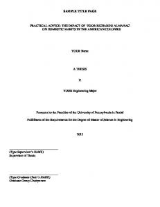

![[SAMPLE TITLE PAGE FORMAT] [Thesis title. Long titles should be ...](https://m.moam.info/img/260x300/sample-title-page-format-thesis-title-long-titles-_59a8e5a41723ddbfc5887b33.jpg)


