Beta Exponentiated Gamma Distribution: Some Properties and Estimation Navid Feroze Government Post Graduate College Muzaffarabad Azad Kashmir, Pakistan
[email protected]
Ibrahim Elbatal Department of Mathematics and Statistics - College of Science Al Imam Mohammad Ibn Saud Islamic University, Saudi Arabia
[email protected]
Abstract The exponentiated gamma (EG) distribution is one of the important families of distributions in lifetime tests. In this paper, a new generalized version of this distribution which is called the beta exponentiated gamma (BEG) distribution has been introduced. The new distribution is more flexible and has some interesting properties. A comprehensive mathematical treatment of the BEG distribution has been provided. We derived the rth moment and moment generating function for this distribution. Moreover, we discussed the maximum likelihood estimation of this distribution under a simulation study.
Keywords: Beta distribution; Hazard function; Exponentiated gamma distribution; Maximum likelihood estimation; Moments. 1. Introduction Gamma distributions are some of the most popular models for hydrological processes. One of the important families of distributions in lifetime tests is the exponentiated gamma (EG) distribution. The exponentiated gamma (EG) distribution has been introduced by Gupta et al. (1998), which has cumulative distribution function (CDF) and a probability density function (pdf) of the form, respectively;
G( x, , ) 1 e x (1 x) , 0, 0 and x 0
(1)
where and are scale and shape parameters respectively. The corresponding probability density function (pdf) is given by 1
g ( x, , ) 2 xe x 1 e x (1 x)
(2)
Shawky and Bakoban (2008) discussed the exponentiated gamma distribution as an important model of life time models and derived Bayesian and non-Bayesian estimators of the shape parameter, reliability and failure rate functions in the case of complete and type-II censored samples. In addition, the order statistics from exponentiated gamma distribution and associated inference was discussed by Shawky and Bakoban (2009). Ghanizadeh, et al. (2011), dealt with the estimation of parameters of the exponentiated gamma (EG) distribution with presence of outliers. The maximum likelihood and moment of the estimators were derived. These estimators are compared empirically using Pak.j.stat.oper.res. Vol.XII No.1 2016 pp141-154
Navid Feroze, Ibrahim Elbatal
Monte Carlo simulation. Singh et al. (2011) proposed Bayes estimators of the parameter of the exponentiated gamma distribution and associated reliability function under general entropy loss function for a censored sample. The proposed estimators were compared with the corresponding Bayes estimators obtained under squared error loss function and maximum likelihood estimators through their simulated risks. Khan and Kumar (2011) established the explicit expressions and some recurrence relations for single and product moments of lower generalized order statistics from exponentiated gamma distribution. Sanjay et el. (2011) proposed Bayes estimators of the parameter of the exponentiated gamma distribution and associated reliability function under general entropy loss function for a censored sample. Feroze and Aslam (2012) introduced Bayesian analysis of exponentiated gamma distribution under type II censored samples. Recently, Parviz et al. (2013) discussed classical and Bayesian estimation of parameters on the generalized exponentiated gamma distribution. Consider starting from the CDF G( x) of a random variable, Eugene et al. (2002) defined a generalized class of distributions by F ( x)
1 G ( x ) (1 a ) b 1 0 w (1 w) dw B ( a, b)
(3)
where a 0 and b 0 are two additional parameters whose role is to introduce skewness and to vary tail weight. And
B(a, b) 0w(1a ) (1 w)b1 dw 1
(4)
is the beta function. The application of the X G 1 (V ) to V B(a, b) yields X with CDF (2). The class of generalized distributions (3) has been receiving considerable attention over the last years, in particular, after the recent studies by Eugene et al. (2002) and Jones (2004). Eugene et al. (2002) introduced what is known as the beta normal ( BN ) distribution by taking G( x) in (3) to be the CDF of the normal distribution and derived some of its first moments. Many authors considered various forms of G and studied their properties: Nadarajah and Kotz (2004) introduced the beta Gumbel ( BGu ) distribution by taking G( x) to be the CDF of the Gumbel distribution and provided closed form expressions for the moments, the asymptotic distribution of the extreme order statistics and discussed the maximum likelihood estimation procedure. Nadarajah and Gupta (2004) introduced the beta Frechet (BFr) distribution, and Cordeiro et al. (2008) (Beta Weibull distribution), Nadarajah and Kotz (2006) (Beta Exponential distribution), Akinsete et al. (2008) (Beta Pareto distribution), Silva et al. (2010) (Beta Modified Weibull distribution), Mahmoudi (2011) (Beta generalized Pareto distribution), Singla et al. (2012) (Beta generalized Weibull distribution), Cordeiro et al. (2012) (Beta generalized gamma distribution) and Cordeiro et al. (2012) (Beta generalized normal distribution). Jafari and Mahmoudi (2012) introduced beta generalized exponential distribution. Recently, Cordeiro et al. (2013) introduced the properties of beta exponentiated weibull distribution. The properties of F ( x) for any beta G distribution defined from a parent G( x) in Equation (3) could, in principle, follow from the 142
Pak.j.stat.oper.res. Vol.XII No.1 2016 pp141-154
Beta Exponentiated Gamma Distribution: Some Properties and Estimation
properties of the hyper geometric function which are well established in the literature; see, for example, Section 9.1 of Gradshteyn and Ryzhik (2000). We can write the Equation (3) by F ( x) IG ( x ) (a, b)
where I y (a, b)
1 B( a,b)
(4) (1 a )
y
0w
(1 w)b1 dw denotes the incomplete beta function ratio, i.e.
the CDF of the beta distribution with parameters a and b . For general a and b , we can express (4) in terms of the well-known hyper geometric function defined by
2 F1 ( , , ; x) i 0
where
F ( x)
( )i ( )i i x, ( )i i !
( ) ( 1)...( i 1)
i G( x) aB ( a , b )
2
denotes the
ascending factorial.
We obtain
F1 (a,1 b, a 1; G( x)) . The properties of F ( x) for any beta G
distribution defined from a parent G( x) in (3) could, in principle, follow from the properties of the hyper geometric function which are well established in the literature; see, for example, Section 9.1 of Gradshteyn and Ryzhik (2000). The probability density function (pdf) corresponding to (3) can be put in the form g ( x) b 1 G( x)a 1 1 G( x) , B ( a, b)
f ( x)
we noted that f ( x) will be most tractable when the CDF G( x) and pdf g ( x) dxd G( x) have simple analytic expressions. Except for some special choices for G( x) in Equation (3), as is the case when G( x) is given by Equation (1), it seems that the pdf f ( x) will be difficult to deal with in generality. Now we introduce the four parameter beta exponentiated Gamma ( BEG) distribution by taking G( x) in (3) to be the CDF (1). The CDF of the BEG distribution is given by F ( x)
1e x (1 x ) 1 w(1a ) (1 w)b 1 dw, x 0 0 B ( a, b)
(5)
for a 0, b 0 , 0 and 0 . The pdf and hazard rate function of the new distribution are, respectively
f ( x)
2 xe x
a 1
1 e x (1 x) B ( a, b)
1 1 e x (1 x)
b 1
,x 0
(6)
and
h( x )
f ( x) 1 F ( x)
2 xe x 1 e x (1 x)
Pak.j.stat.oper.res. Vol.XII No.1 2016 pp141-154
B ( a, b) I
a 1
1 1 e x (1 x)
1 1 e x (1 x )
( a, b)
b 1
,
143
Navid Feroze, Ibrahim Elbatal fx
fx
0.010
0.010
Parameters
0.008
0.008
Parameters
P1
P1 0.006
P2 0.006
P3
P2 P3
0.004
P4
P4
0.004
0.002
20
40
60
80
x
100
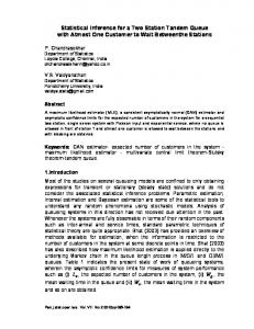
Fig. 1: Curves of pdf for different parametric values P1 => (a = 0.2, b = 0.1, λ = 0.1, θ = 0.1) P2 => (a = 0.2, b = 0.1, λ = 0.1, θ = 0.5) P3 => (a = 0.2, b = 0.1, λ = 0.1, θ = 1) P4 => (a = 0.2, b = 0.1, λ = 0.1, θ = 2)
fx 0.030
20
40
60
80
100
120
x
140
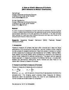
Fig. 3: Curves of pdf for different parametric values P1 => (a = 0.2, b = 0.1, λ = 0.1, θ = 0.1) P2 => (a = 0.2, b = 0.1, λ = 0.1, θ = 0.5) P3 => (a = 0.2, b = 0.1, λ = 0.1, θ = 10) P4 => (a = 0.2, b = 0.1, λ = 0.1, θ = 20)
fx
0.04 0.025 0.020
Parameters
0.03
Parameters
P1 0.015
P1
P2
P2
0.02
P3
0.010
P3
P4
P4 0.01
0.005
20
40
60
80
100
120
140
x
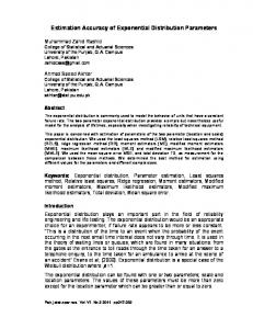
Fig. 2: Curves of pdf for different parametric values P1 => (a = 0.2, b = 0.5, λ = 0.1, θ = 0.1) P2 => (a = 0.2, b = 0.5, λ = 0.1, θ = 0.5) P3 => (a = 0.2, b = 0.5, λ = 0.1, θ = 10) P4 => (a = 0.2, b = 0.5, λ = 0.1, θ = 20)
20
40
60
80
100
x
Fig. 4: Curves of pdf for different parametric values P1 => (a = 0.1, b = 0.1, λ = 0.1, θ = 10) P2 => (a = 0.5, b = 0.5, λ = 0.1, θ = 10) P3 => (a = 0.9, b = 0.9, λ = 0.1, θ = 10) P4 => (a = 2, b = 2, λ = 0.1, θ = 10)
The probability density function in Equation (6) does not involve any complicated function. If X is a random variable with pdf (6), we write X BEG(a, b, , ) . The BGE distribution generalizes some well-known distributions in the literature. If a b 1 , we get Exponentiated gamma distribution, also when the shape parameter a b 1 in both (1) and (2) give the CDF and pdf of gamma distribution with shape parameter 2 and scale parameter 1 i.e. G(2,1) . For more details about this distribution, see: Shawky and Bakoban (2008). The rest of the paper is organized as follows. In section 2, we demonstrate that the ( BEG) density function can be expressed as a linear combination of the exponentiated gamma. This result is important to provide mathematical properties of the BEG model directly from those properties of the exponentiated gamma distribution. In section 3, we 144
Pak.j.stat.oper.res. Vol.XII No.1 2016 pp141-154
Beta Exponentiated Gamma Distribution: Some Properties and Estimation
discussed some important statistical properties of the ( BEG) distribution such as quantile, and the ordinary moments and measures of skewness and kurtosis. The distribution of the order statistics is expressed in section 4. The maximum likelihood estimates of the four parameter index to the distribution are presented in section 5. The section 6 contains the simulation study. Finally the discussion and conclusion regarding the study have been presented in the section 7. 2. Expansion for the Density Function In this section, we presented two formulae for the CDF of the BEG distribution depending if the parameter b 0 is real non- integer or integer. First, if z 1 and b 0 is real non- integer, we have b 1 j (1) j (b) j (1 z )b1 (1) j z z j !(b j ) j 0 j
(7)
Using the expansion (7) in (5), the CDF of the BEG distribution when b 0 is real non-integer follows
F ( x)
1 e x (1 x ) 1 w(1 a ) (1 w)b 1 dw 0 B ( a, b)
1 e x (1 x ) (b) (1) j wa j 1dw 0 B(a, b) j 0 j !(b j )
and then (a j ) ( a b) (1) j 1 e x (1 x) F ( x) (a) j 0 j !(b j )(a j )
(8)
Equation (8) reveals the property that the CDF of the BEG distribution can be expressed as an infinite weighted sum of CDFs of EG distributions, F ( x)
(a b) (1) j G( x, , (a j )) . (a) j 0 j !(b j )(a j )
when b 0 is integer, using the expansion (7) in (5) , we get F ( x)
(a j ) 1 b1 b 1 (1) j 1 e x (1 x) B ( a, b) j 0 j ( a j )
(9)
Again, the same property of Equation (8) holds but now the sum is finite. Expression (8) and (9) are the main results of this section. Also the pdf (6) can be expressed in mixture from in terms of CDFs of the exponentiated gamma distributions, if b is real noninteger, we have f ( x)
2 xe x B ( a, b)
G( x, , a 1) j 0
Pak.j.stat.oper.res. Vol.XII No.1 2016 pp141-154
(1) j G ( x, , j ) j !(b j )
(10)
145
Navid Feroze, Ibrahim Elbatal
and if b is integer, then f ( x)
2 xe x
b 1 b 1 G( x, , a 1) (1) j G ( x, , j ). B ( a, b) j 0 j
3. Statistical Properties This section is devoted to studying statistical properties of the ( BEG) distribution, specifically the quantile function, moments and moment generating function 3.1 Quantile Function The quantile xq of the ( BEG) distribution can be easily given as F ( xq ) I
1e x (1 x )
( a,b)
(a, b) P( X xq )
(11)
where ( xq )( BEG ) F 1 (u), is given by the following relation 1
e x (1 x) 1 I u(1a , b )
(12)
3.2 Moments In this subsection we discussed the rth moment for ( BEG) distribution. Moments are necessary and important in any statistical analysis, especially in applications. It can be used to study the most important features and characteristics of a distribution (e.g., tendency, dispersion, skewness and kurtosis). Theorem (3.1) , ( , ,a ,b ) then the rth moment of X is given by the
If X has BEG(, x) following
r ( x)
m 2
(1) B ( a, b)
j k
j 0 k 0 m 0
b1 ( j a ) 1 k (r m 2) r m 2 j k m (k 1)
(13)
Proof: Let X be a random variable with density function (10). The rth ordinary moment of the ( BEG) distribution is given by
r ( x) E ( X r ) 0 x r f ( x, )dx
2 xe x B ( a, b)
r 1 0
x
r 1 x 0
C x e
146
1 e x (1 x)
1 e x (1 x)
a 1
a 1
1 e x (1 x)
1 e x (1 x)
b 1
dx
b 1
dx
Pak.j.stat.oper.res. Vol.XII No.1 2016 pp141-154
Beta Exponentiated Gamma Distribution: Some Properties and Estimation
where
C
2
,
B ( a, b)
setting 1 e x (1 x)
j b 1 (1) j 1 e x (1 x) j 0 j
b 1
(14)
then ( j a ) 1 b1 r 1 x x 0 x e 1 e (1 x) j
r ( x) C (1) j j 0
but ( j a ) 1
1 e x (1 x)
( j a )1 kx k (1)k e (1 x) k 0 k
(15)
then
b 1 ( j a ) 1 r 1 ( k 1) x (1 x)k dx 0 x e j k
r ( x) C (1) j k j 0 k 0
again k (1 x) k ( x)m m 0 m
(16)
Thus the rth moment is given by
b 1 ( j a ) 1 k m r m 1 ( k 1) x e dx 0 x j k m
r ( x) C (1) j k j 0 k 0 m 0
C
m
(1)
j k
j 0 k 0 m 0
m 2
(1) B ( a, b)
b 1 ( j a ) 1 k (r m 2) r m 2 j k m (k 1)
j k
j 0 k 0 m 0
(17)
b 1 ( j a ) 1 k (r m 2) r m2 j k m (k 1)
which completes the proof . Based on the first four moments of the ( BEG) distribution, the measures of skewness A() and kurtosis k () of the ( BEG) distribution can obtained as A()
3 ( ) 31 ( ) 2 ( ) 213 ( )
k ( )
4 ( ) 41 ( ) 3 ( ) 612 ( ) 2 ( ) 314 ( )
3
2 ( ) 12 ( ) 2
,
and
2 ( ) 12 ( )
Pak.j.stat.oper.res. Vol.XII No.1 2016 pp141-154
2
.
147
Navid Feroze, Ibrahim Elbatal
3.3. Moment Generating function In this subsection we derived the moment generating function of ( BEG) distribution. Theorem (3.2): If X has ( BEG) distribution, then the moment generating function M X (t ) has the following form
M X (t )
m 2
(1) B ( a, b)
j k
j 0 k 0 m 0
b1 ( j a )1 k (m 2) m 2 j k m (k 1) t
(18)
Proof. We start with the well known definition of the moment generating function given by
M X (t ) E (etx ) etx f BEG ( x, )dx 0
(19)
xe 2
x
r 1
0 x
B ( a, b)
1 e x (1 x)
a 1
1 e x (1 x)
b 1
dx
substituting from (14) and (15) into (19) we get
M X (t )
m 2
(1) B ( a, b)
j k
j 0 k 0 m 0
m 2
(1) B ( a, b)
j k
j 0 k 0 m 0
b 1 ( j a ) 1 k m 1 x ( k 1)t dx 0 x e j k m b 1 ( j a ) 1 k (m 2) . m 2 j k m (k 1) t
Which completes the proof. 4. Distribution of the order statistics In this section, we derive closed form expressions for the pdfs of the rth order statistic of the ( BEG) distribution, also, the measures of skewness and kurtosis of the distribution of the rth order statistic in a sample of size n for different choices of n; r are presented in this section. Let X1 , X 2 ,..., X n be a simple random sample from ( BEG) distribution with pdf and CDF given by (6) and (9), respectively. Let X1 , X 2 ,..., X n denote the order statistics obtained from this sample. We now give the probability density function of X r : n , say f r : n ( x, ) and the moments of X r : n , r 1, 2,..., n . Therefore, the measures of skewness and kurtosis of the distribution of the X r : n are presented. The probability density function of X r : n is given by
f r : n ( x, )
148
1 r 1 nr F ( x, ) 1 F ( x, ) f ( x, ) B(r , n r 1)
(20)
Pak.j.stat.oper.res. Vol.XII No.1 2016 pp141-154
Beta Exponentiated Gamma Distribution: Some Properties and Estimation
where F ( x, ) and f ( x, ) are the CDF and pdf of the ( BEG) distribution given by (6), (9), respectively, and B(.,.) is the beta function, since 0 F ( x, ) 1 , for x 0 , by using the binomial series expansion of 1 F ( x, )
nr
1 F ( x, )
nr
, given by
j nr (1) j F ( x, ) , j 0 j
nr
we have nr nr r j 1 f r : n ( x, ) (1) j f ( x, ) F ( x, ) j 0 j
(21)
substituting from (6) and (9) into (21), we can express the kth ordinary moment of the
rth order statistics X r : n say E ( X rk : n ) as a linear combination of the kth moments of the ( BEG) distribution with different shape parameters. Therefore, the measures of skewness and kurtosis of the distribution of X r : n can be calculated. 5. Estimation and Inference In this section, we determined the maximum likelihood estimates (MLEs) of the parameters of the ( BEG) distribution from complete samples only. Let X1 , X 2 ,..., X n be a random sample of size n from BEG( , , a, b) The likelihood function for the vector of parameters ( , , a, b) can be written as
Lf ( x(i ) , ) in1 f ( x(i ) , )
2
xi a 1 in1 xi e i1 in1 1 e xi (1 xi ) n i 1 B(a, b) n
n
in1 1 1 e x (1 x)
b 1
.
Taking the log-likelihood function for the vector of parameters ( , , a, b) we get
log L n log 2n log n log ( a b) n log ( a) n log (b) n
n
n
i 1
i 1
i 1
log( xi ) x(i ) ( a 1) log 1 e xi (1 xi ) n
(b 1) log 1 1 e x (1 x) i 1
Pak.j.stat.oper.res. Vol.XII No.1 2016 pp141-154
(22)
149
Navid Feroze, Ibrahim Elbatal
The log-likelihood can be maximized either directly or by solving the nonlinear likelihood equations obtained by differentiating (22). The components of the score vector are given by n 1 e log L n n log 1 e xi (1 xi ) (b 1) i 1 i 1
xi
x (1 xi ) log 1 e i (1 xi ) (23) xi 1 1 e (1 xi )
x
x
2 i x 1 e i (1 xi ) n n xi e xi2e i log L 2n n xi ( a 1) ( b 1) i 1 1 e xi (1 x ) i 1 xi i 1 1 1 e (1 xi ) i
1
n log L n (a b) n (a) log 1 e xi (1 xi ) i 1 a
(24)
(25)
and
n log L n (a b) n (b) log 1 1 e x (1 x) i 1 b
(26)
where (.) is the digamma function. We can find the estimates of the unknown parameters by maximum likelihood method by setting these above non-linear equations (23) - (26) to zero and solve them simultaneously. As the closed for expressions for the estimators cannot be derived we have obtained the estimated values numerically. 6. Simulation Study The simulation study has been conducted in order to have the numerical estimates for the parameters of the beta exponentiated gamma distribution. The samples of sizes 20, 50 and 100 have been drawn from the distribution under 1000 replications. Different combinations of the parameters {(θ, λ, a, b) = (0.1, 0.1, 0.1, 0.1), (10, 10, 10, 10), (100, 100, 100, 100), (100, 0.1, 0.1, 0.1), (0.1, 100, 0.1, 0.1), (0.1, 0.1, 100, 0.1) and (0.1, 0.1, 0.1, 100)} have been assumed to investigate and compare the performance of the estimates. The amounts of variances for the estimates of each parameter have been reported in the parenthesis in the tables.
150
Pak.j.stat.oper.res. Vol.XII No.1 2016 pp141-154
Beta Exponentiated Gamma Distribution: Some Properties and Estimation
Table 1: MLE and variances for the different values of θ, λ, a and b (θ, λ, a, b)
n 20
(0.1, 0.1, 0.1, 0.1)
50 100 20
(10, 10, 10, 10)
50 100 20
(100, 100, 100, 100)
50 100
ˆ
ˆ
aˆ
bˆ
0.13108 (0.06584) 0.12491 (0.04259) 0.11942 (0.03170) 13.22759 (1.41686) 12.47687 (0.87680) 11.23081 (0.42148) 119.03190 (8.01888) 116.05310 (5.19113) 108.16250 (3.18452)
0.14014 (0.03661) 0.12660 (0.02819) 0.11516 (0.02112) 14.03771 (0.56764) 12.44025 (0.43504) 11.15227 (0.30988) 0.13571 (0.03387) 0.13531 (0.02719) 0.11077 (0.01944)
0.13187 (0.05695) 0.12619 (0.04881) 0.11415 (0.03270) 13.25134 (1.23619) 12.48110 (0.90339) 10.98506 (0.49297) 0.14701 (0.05143) 0.13362 (0.04399) 0.11784 (0.03099)
0.14116 (0.07296) 0.12884 (0.03539) 0.11959 (0.02905) 14.23258 (1.55018) 12.79116 (0.53345) 11.38695 (0.40885) 0.13405 (0.06863) 0.12747 (0.03368) 0.11017 (0.02812)
Table 2: MLE and variances for the different values of θ, λ, a and b (θ, λ, a, b)
n 20
(100, 0.1, 0.1, 0.1)
50 100 20
(0.1, 100, 0.1, 0.1)
50 100 20
(0.1, 0.1, 100, 0.1)
50 100 20
(0.1, 0.1, 0.1, 100)
50 100
ˆ
ˆ
aˆ
bˆ
0.12729 (0.06160) 0.12255 (0.03967) 0.11591 (0.02945) 0.12863 (0.06191) 0.12030 (0.03884) 0.11545 (0.02883) 0.12962 (0.06025) 0.12254 (0.03974) 0.11788 (0.03011) 119.03190 (8.01888) 116.05310 (5.19113) 108.16250 (3.18452)
133.27437 (4.40349) 123.70440 (3.42400) 109.72504 (2.65382) 0.13705 (0.03442) 0.12189 (0.02541) 0.11119 (0.01930) 0.13828 (0.03408) 0.12514 (0.02575) 0.11305 (0.01976) 0.13571 (0.03387) 0.13531 (0.02719) 0.11077 (0.01944)
0.12940 (0.05355) 0.12153 (0.04452) 0.11035 (0.02974) 125.40299 (6.84961) 123.29934 (5.92897) 108.76204 (4.10896) 0.12931 (0.05395) 0.12404 (0.04628) 0.11271 (0.02989) 0.14701 (0.05143) 0.13362 (0.04399) 0.11784 (0.03099)
0.13805 (0.06860) 0.12404 (0.03190) 0.11547 (0.02654) 0.13707 (0.06826) 0.12640 (0.03296) 0.11607 (0.02700) 135.38948 (8.72897) 124.02699 (3.98361) 114.50213 (3.46003) 0.13405 (0.06863) 0.12747 (0.03368) 0.11017 (0.02812)
Pak.j.stat.oper.res. Vol.XII No.1 2016 pp141-154
151
Navid Feroze, Ibrahim Elbatal
Table 3:
Skewness and Kurtosis for the distribution using different parametric values
Parametric Space Coefficient of Skewness Coefficient of Kurtosis
a = 0.2, b = 0.5, λ = 0.1, θ = 0.1
a = 0.2, b = 0.1, λ = 0.1, θ = 1
a = 0.9, b = 0.9, λ = 0.1, θ = 10
a = 2, b = 2, λ = 10, θ = 10
0.30
0.63
0.83
0.14
3.71
4.08
3.26
4.31
We have used the real life data set regarding the breaking strengths of 64 single carbon fibers of length 10, presented Lawless (2003) for the analysis in the following table. Table 4: MLE and variances for θ, λ, a and b using real life data set Parameters
ˆ
ˆ
aˆ
bˆ
MLE and variances
18.4721 (3.1269)
3.8731 (1.8673)
0.9848 (0.3919)
0.5781 (0.2170)
7. Discussion and Conclusion The aim of this paper is to introduce a new distribution named beta exponentiated gamma distribution and to discuss its properties. The maximum likelihood estimates for the parameters of the distribution has been obtained. Tables 1-2 show that the estimated values of the parameters converge to the true values as sample size increases. The larger choice of the true parametric values inflates the variances associated with the estimates of each parameter; however this is natural consequence of the lager values of the parameters. Keeping the value of one of the parameter specified, the smaller choice of other parametric values imposes a positive impact on the estimation of the specified parameter. On the whole, the proposed estimators are consistent and can be used in various real life situations. The table 3 suggests that the distribution is positively skewed and leptokurtic under different parametric values. In addition the newly introduced distribution is much more flexible than its available counterparts, so it will be very useful for modeling failure time data. The flexibility of the beta exponentiated gamma model, however, occurs at the cost of its increased complexity, but a comprehensive programming in different computer software can tackle with these complexities. In future this work can be extended by considering the analysis of the distribution under censored samples. References 1.
Akinsete, A., Famoye, F. and Lee, C. (2008). The beta-Pareto distribution, Statistics, 42(6), 547-563.
2.
Cordeiro, G. M., Gomez, A. E., De-Silva, C. Q. and Ortega, E. E. M. (2013). The beta exponentiated Weibull distribution, Journal of Statistical Computation and Simulation, 83(1), 114-138.
3.
Cordeiro, G. M., Castellaresb, F., Montenegrob, L. and Castro, M. (2012). The beta generalized gamma distribution, Statistics, 35, 1-13.
152
Pak.j.stat.oper.res. Vol.XII No.1 2016 pp141-154
Beta Exponentiated Gamma Distribution: Some Properties and Estimation
4.
Cintra, R. J., Rago, L. C., Cordeiro, G. M. and Nascimento, A. D. C. (2014). Beta generalized normal distribution with an application for SAR image processing, Statistics, 48(2), 279-294.
5.
Cordeiro, G. M., Simas, A. B. and Stosic, B. D. (2008). Explicit expressions for moments of the beta Weibull distribution, Preprint:/arXiv:0809.1860v1S.
6.
Cordeiro, G. M., Gomes, A. E., de Silva, C. Q. and Ortega, E. M. M. (2013). The beta exponentiated Weibull distribution, Journal of Statistical Computation and Simulation, 83(1), 114-138.
7.
Eugene, N., Lee, C., and Famoye, F. (2002). Beta-normal distribution and its applications, Communication in Statistics- Theory and Methods, 31, 497-512.
8.
Ghanizadeh, A, Pazira, H. and Lot,. R (2011). Classical Estimations of the Exponentiated Gamma Distribution Parameters with Presence of K Outliers, Australian Journal of Basic and Applied Sciences, (5)3, 571-579.
9.
Gradshteyn I.S. and Ryzhik, I. M. (2000). Table of Integrals, Series, and Products, Academic Press, New York.
10.
Gupta, R. C, Gupta R. D. and Gupta, P. L. (1998). Modeling Failure Time Data by Lehman Alternatives, Commun. Statist.-Theory, Meth., 27(4), 887-904.
11.
Jafari, A. and Mahmoudi, E. (2012) Beta-Linear Failure Rate Distribution and its Applications. rXiv:1212.5615.
12.
Jones, M. C. (2004). Family of distributions arising from distribution of order statistics. Test, 13, 1- 4.
13.
Khan R. and Kumar, D. (2011). Lower Generalized Order Statistics from Exponentiated Gamma Distribution and Its Characterization, Prob Stat Forum, 4, 25-38.
14.
Lawless, J. F. (2003). Statistical Models time Data, 2nd Edition. Wiley, New York.
15.
Mahmoudi, E. (2011). The beta generalized Pareto distribution with application to lifetime data, Mathematics and Computers in Simulation, 81(11), 2414-2430.
16.
Nadarajah, S., and Gupta, A. (2004). The beta Frechet distribution, Far East Journal of Theoretical Statistics, 14, 15-24.
17.
Nadarajah, S., and Kotz, S. (2006). The beta exponential distribution, Reliability Engineering and System Safety, 91, 689-697.
18.
Nadarajah, S and Kotz, S. (2004). The beta Gumbel distribution, Math. Problems Eng., 10, 323--332.
19.
Feroze, N. and Aslam, M. (2012). Bayesian Analysis of Exponentiated Gamma Distribution under Type II Censored Samples, International Journal of Advanced Science and Technology, 49, 37-46.
20.
Parviz, N, Rasoul,. L. and Hossein, V. (2013). Classical and Bayesian estimation of parameters on the generalized exponentiated gamma distribution, Scientific Research and Essays, 8(8), 309-314.
Pak.j.stat.oper.res. Vol.XII No.1 2016 pp141-154
153
Navid Feroze, Ibrahim Elbatal
21.
Sanjay. K., Umesh, S. and Dinesh, K. (2011). Bayesian Estimation of the Exponentiated Gamma Parameter and Reliability Function Under Asymptotic Symmetric Loss Function. Revesta -Statistical Journal, 9(3), 247-260.
22.
Shawky, A. I. and Bakoban, R. A. (2008). Bayesian and Non-Bayesian Estimations on the Exponentiated Gamma Distribution, Applied Mathematical Sciences, 2(51), 2521-2530.
23.
Shawky, A. I. and Bakoban, R. A. (2009). Order Statistics from Exponentiated Gamma Distribution and Associated Inference, Int. J. Contemp. Math. Sciences, 4(2), 71-91.
24.
Silva, G. O. Ortega, E. M. M. and Cordeiro, G. M. (2010). The beta modified Weibull distribution, Lifetime Data Analysis, 16, 409-430.
25.
Singla, N., Kanchan, Jain. and Suresh, K. (2012). The Beta Generalized Weibull distribution, Properties and applications, Reliability Engineering & System Safety, 102, 5-15.
154
Pak.j.stat.oper.res. Vol.XII No.1 2016 pp141-154