statistics, census, sampling surveys based on list frame or area frame and ..... or have been set up in close collaboration with the MARS Project: Greece, Spain, Portugal, ..... In the mountain stratum, only the pre-sample segments coming from.
SAMPLING FRAMES OF SQUARE SEGMENTS
Francisco Javier Gallego MARS Project, Institute for Remote Sensing Applications JRC, 21020 Ispra (Varese) Italy
Report EUR 16317, 1995, Office for Publications of the E.C. Luxembourg. ISBN 92-827-5106-6
1995
TABLE OF CONTENTS
1.
SOME APPROACHES TO AGRICULTURAL STATISTICS 1.1 Village Statistics 1.2 Census of Farms 1.2.1 Defining a farm 1.2.2 Measuring farm size 1.2.3 Validity of census data 1.3 Sampling Surveys
2.
3.
4
2.1 Finite and Infinite Sampling Frames 2.2 Sampling Farms from a List Frame 2.3 Area Frame Sampling with Direct Observation. 2.3.1 Area Frames of Segments 2.3.2 Area Frames of Points 2.4 Sampling Farms in an Area Frame 2.4.1 Open, closed, and weighted segment estimators 2.4.2 Sub-sampling farms for a weighted estimator 2.5 Sampling Errors and Non-Sampling Errors 2.6 Area frames for environmental surveys.
4 4 4 5 5 6 6 6 6 6
SAMPLING FRAMES OF CADASTRAL SEGMENTS
AREA FRAMES OF SEGMENTS WITHOUT PHYSICAL LIMITS 4.1 4.2 4.3
5.
1 1 2 2 2 3
SAMPLING FRAMES IN AGRICULTURE
3.1 Defining Cadastral Segments 3.1.1 Primary and secondary sampling units
4.
1
Why Use Segments without Physical Boundaries? Area Frame Based on Square Segments Segment Location and Shape Errors in an Area Sampling Frame on a square grid.
7 7 7
9 9 9 10
SAMPLING IN AN AREA FRAME BASED ON SQUARE SEGMENTS 12 5.1 Simple random sampling 5.2 Sampling with a distance threshold 5.3 Sampling Square Segments by Square Blocks. 5.3.1 Non aligned sample 5.3.2 Sampling square segments repeating a fixed pattern. 5.3.3 Systematic aligned sampling with a distance threshold. 5.4 Estimates and their Precision
12 13 13 13 14 14 16
6. PRACTICAL CHOICES TO SET UP AN AREA FRAME OF SQUARE SEGMENTS. 18 6.1 Some Restrictions of Ground Survey Material 6.2 Segment size 6.2.1 Size reduction for particular segments when fields are small. 6.2.2 Effect of a general segment size reduction in a stratum. 6.3 Sampling rate.
18 20 20 21 23
7.
STRATIFICATION OF AN AREA FRAME
24
7.1 Stratification Tools for Area Frames 24 7.1.1 Geographic Information Systems (GIS) 24 7.1.2 High Resolution Satellite Images (Landsat TM or SPOT). 24 7.1.3 Low resolution Satellite Images (NOAA-AVHRR) 24 7.1.4 Clustering Segments 25 7.2 Examples of Stratification in Different Countries 25 7.2.1 Région Centre (France) 25 7.2.2 Emilia Romagna (Italy) 25 7.2.3 Castilla y León (Spain) 26 7.2.4 Bayern (Germany) 26 7.2.5 Makedonia (Greece) 26 7.2.6 An example of NASS stratification (U.S.A.) 27 7.3 Systematic Sampling with a Distance Threshold in a Stratified Area Sampling Frame on a Square Grid. 27 7.4 Estimators for Stratified Sampling and their Precision 29 7.4.1 Post-stratification correction 30 7.5 Efficiency of the Stratification 30 7.6 Dealing with Segments that Straddle Boundaries 30 7.6.1 Segments on the border of the region 30 7.6.2 Segments across strata boundaries 31
8. EXPECTED PRECISION OF AREA ESTIMATES FROM A GROUND SURVEY WITH SQUARE SEGMENTS 32 9. PLANNING A GROUND SURVEY BASED ON SQUARE SEGMENT SAMPLING 36 9.1 Photographs and Maps 9.2 Crop Calendar and Dates for the Ground Survey 9.3 Surveyors. 9.4 9.5 Digitising Equipment and Software for Calculation of Estimates 9.5.1 TTS and TTS+ 9.5.2 AIS_STIM and RIESLYNG 9.6 Approximate Time Schedule.
10. SAMPLING POINTS CLUSTERED BY SQUARE SEGMENTS 10.1
Cost Efficiency of Point and Segment Surveys
11. SEGMENT SURVEY AND FARM SURVEY.
36 36 36 Stratification 37 37 37 38
37
39 39
41
11.1 Sampling Farms by Points in an Area Frame of Square Segments 41 11.1.1 Field work 42 11.1.2 Estimates based on farms sampled by points 11.1.3 Missing values 44 11.1.4 An example: Czech Republic in 1992 44
12. SOME CONCLUSIONS ON AREA FRAMES OF SEGMENTS WITHOUT PHYSICAL BOUNDARIES 46 REFERENCES
47
GLOSSARY
50
42
LIST OF FIGURES
Figure 1: A sample of square segments. Figure 2: Sampling cadastral segments through primary sampling units. Figure 3: Segment without physical boundaries. Figure 4: Square grid on a small region. Figure 5: Shape and location errors Figure 6: Simple random sample Figure 7: Random sample with a distance threshold. Figure 8: Non aligned sample by square blocks Figure 9: Random pattern in a block Figure 10: Aligned sample by repeating a pattern Figure 11: Sampling a pattern in a block with a distance threshold Figure 12: Aligned sample with a distance threshold. Figure 13: Sampling grid avoiding map limits Figure 14: Sample with 4 segments per block Figure 15:Regular grid of segments of 700 m on a grid of maps of 3 km Figure 16: Restricted sampling frame Figure 17: Square segment of 400 ha Figure 18: Cutting the segment to a smaller size Figure 19: Ratio of the standard error for different segment sizes over the standard error for segments of 100 ha (Czech Republic, stratum 1). Figure 20: Relative efficiency of the segment size. Figure 21: Stratification in Valladolid-Zamora (Spain) Figure 22: Stratified region. Figure 23: Pattern of 4 segments in a square block Figure 24: Pre-sample Figure 25: Final sample Figure 26: Approximation of a region to a square grid Figure 27: Segment shared by 2 strata. Figure 28: Plot of (coefficient of variation* n ) with the percentage of crops Figure 29 : Plot of the coefficient of variation with the % of the crop or group of crops in the region. Figure 30: Plot of the standard error of the area estimates with the estimated area of the crop. Figure 31: Expected precision with different sample sizes Figure 32: Expected precision (logarithmic scale for y ) Figure 33: Grid of 25 points in a square segment Figure 34: Sampling farms in a segment with a point grid
5 8 9 10 10 12 12 13 14 14 15 15 18 19 19 20 21 21 22 22 26 28 29 29 29 31 31 33 33 34 35 35 39 41
1
1.
Some Approaches to Agricultural Statistics
Statistical services rely on different methods, resulting from both historical reasons and available techniques, to provide reliable figures. Most often, the applied systems are based on: village statistics, census, sampling surveys based on list frame or area frame and administrative by-products [Meyer-Roux, 1987]. These will likely be modified in the forthcoming years by the impact of new technologies, such as Geographic Information Systems and Remote Sensing. In the present report, we try to review some of the procedures for agricultural statistics, mainly in use in the countries of the European Community. 1.1 Village Statistics The basic unit is an administrative unit (e.g. municipality, small agricultural region, parish) which includes a number of farmers as well as a territory. All data can be retrieved for agriculture, environment, industry or education. In the case of agriculture, this task is usually performed by local administrators or agricultural organisations. The data collectors give subjective estimates of area and possibly of production per crop type. Additional data on other farm characteristics, such as equipment and education, can also be procured. Data processing is relatively simple, since no sampling is involved and the number of units is small in comparison to the number of farmers or the number of agricultural fields. The whole national territory can be covered, if a stable structure of local correspondents has been set up. Village, municipality and parish statistics are commonly used in many developing countries, but also in developed ones. Within the European Community, Greece employs such an approach to produce some of its statistics. Spain has widely used this system, which is progressively being phased out by estimates based on area frame sampling or list sampling. However, it is unlikely that this procedure can be eliminated in the short term for minor crops, particularly when concentrated in specific areas. Village statistics are useful as an alternative, when it is difficult to collect data from farmers or from other means, such as direct ground observations. In some countries, getting data from farmers can be difficult, because they are not adequately trained to provide reliable figures, are difficult to locate or unwilling to answer to questions on their production or income. Village statistics are cheap to produce, but are a burden to local administrations. At times it is difficult to obtain data, if these local entities do not co-operate. In general, estimating agricultural magnitudes in this manner yields results of rather poor quality. The main problem is that often the bias due to subjectiveness is systematically in the same direction. For example, if there is a strong change in crop area (e.g. increase by 100%), local correspondents tend to be conservative and report the change in a smoothed way (saying for instance that the increase has been 50%). Reports by local experts are not easy to substitute when figures are requested for very small administrative units, in which it would be too expensive to draw a large enough sample for an unbiased estimate with a decent coefficient of variation. Possible systematic biases might be eliminated or reduced by combining this information with data from a sampling survey. 1.2 Census of Farms Producing an exhaustive list of farms in a country or region is an obvious way to compute crop areas, yields or other information. Only few, small countries can afford a yearly farm census. Most countries carry out this operation with an interval of 5 to 10 years. In this case, the census provides a sampling frame for yearly surveys. In northern Europe, where the educational level of farmers is
2 relatively high, a census can be made by mail or telephone, possibly completed by a field survey to identify new farms or to collect data from non-respondents. In southern Europe or in developing countries with a large number of small farms, a huge amount of work is involved to interview all farmers. 1.2.1 Defining a farm In practice, the definition of the farm as a unit is not always straightforward. A farm is usually defined as an agricultural production unit with a single management and a size beyond a certain threshold. Some problems are related to the term "production unit", e.g. when a farmer partially manages his activity alone and partially in association with others. The main question for the definition of a farm is the way to measure the size and the choice of a size threshold to distinguish between professionally managed (possibly part-time) and “hobby” farms. 1.2.2 Measuring farm size Farm size can be defined through the Utilised Agricultural Area, which does not take into account the heterogeneity of land. A property of 10 or 20 ha in Australia will usually be considered as a hobby farm, but the same area corresponds to an unusually large farm in many other countries. Such a contrast can also appear within a country or a region with a rich irrigated plain and poor, dry pastures in hilly areas. This drawback can be overcome by giving separate weights to different qualities of land. However, this approach cannot properly deal with very intensive cattle farms without agricultural land. An economic criterion may be more useful to measure farm size. Many countries define size by the value of the marketed products in an average year. The EC has set up a measuring system based on the based on the SGM “standard gross margins” (MBS in french for “marges brutes standard”), which are defined as the value of the output less cost of the variable inputs. For the calculation of farm size, approximate average values are provided for each province or county per hectare of crop or per unit of livestock [Eurostat, 1986; Mc Clintock, 1990]. The threshold for a farm to be considered “professional”, rather than hobby or subsistence farm, by the European Farm Structure Survey ranges from a standard gross margin of 1,000 ECU for Portugal to 16,000 ECU in the Netherlands. However, this criterion does not necessarily coincide with the standards applied by the member states of the European Community for their national statistics. 1.2.3 Validity of census data Census of farms are made in all EC and most developing countries in accordance with the recommendations of the Food and Agriculture Organisation (FAO). They are suitable to cover all types of statistics related to the farm: crop area, production, livestock and economic parameters. Obviously, data coming from a farm census do not have any sampling error, but the results can have some weaknesses due to several reasons:
Agricultural production from farms under the threshold size may be far from negligible . Farmers are not always able to provide reliable figures on the production of certain items. Farmers may give answers with a systematic bias, if they think their figures may be used for subsidies or tax purposes. Bias can partially be overcome by again interviewing a subsample of farmers [Hood, 1993].
3 1.3
Sampling Surveys
When a census is made every 5 or 10 years, the results obtained directly are clearly not valid for the whole period between censuses. Yearly surveys can be made by a partial observation of the agricultural sector. Sampling theory provides tools to make an objective extrapolation to the whole population by just observing a small part (sample) of the population.
4
2.
Sampling Frames in Agriculture
The first step to select a sample is to define a sampling frame. A frame specifies the elements of a population out of which a sample can be drawn to estimate a certain characteristic of the complete population. 2.1 Finite and Infinite Sampling Frames When the population is finite, the frame may be defined by an explicit list of its elements (for instance a population census, a list of the companies in a country or the set of invoices of a company being audited). In agricultural statistics, this corresponds to sampling farms from a census supposed to contain all the farms of the region surveyed (list frame) or from an area frame of segments limited by physical elements of the landscape (cadastral segments). Sometimes the population is infinite, such as the set of possible values of the duration of a certain event (a phone call for example) or the set of points in a geographical space. Infinite sampling frames can often be considered as finite by allocating a size to each element (considering that a geographic point is a square of 1m2). However, this does not necessarily bring any advantage, since most formulae are easier for sampling in infinite spaces. This would be the situation for agricultural surveys by point sampling in area frames. In many occasions, the frame is finite, but there is no need to build up an explicit list of their elements; this happens, for example, when sampling square segments in an area frame. 2.2 Sampling Farms from a List Frame A list frame is derived from a list of farms from which a sample is drawn. The frame is usually classified according to size and specialisation [Eurostat, 1986]. One main limitation of this type of survey is that the sampling frame (the census) is usually not updated at the time of the sample. Some farms have disappeared, other farms have been created, split or merged, and many have changed size or specialisation. To cope with the incompleteness of the list frame, it can be complemented with area frames, building a multiple frame [Kott and Vogel, 1995, Hartley, 1974]. This approach has been used for example by Statistics Canada. Moreover, the drawbacks mentioned for census apply in general to list frame surveys and appear as non-sampling errors. Finally, another problem related to both census and sampling farms (on a list or area frame) is the response burden placed on farmers, which may lead to inaccurate data or a refusal to answer. Farmers have to respond to more and more questionnaires for administrative or statistical purposes and this can cause a negative attitude towards any type of survey. Hence, it is important that the questionnaires are simple, brief and with an easy-to-read introduction explaining the purpose of the survey [Biemer, 1991; Gower, 1993]. 2.3 Area Frame Sampling with Direct Observation. Area frames provide a different approach to agricultural statistics. The units of an area frame are directly bound to a geographical area. If we know the limits of the region, we will exactly know the elements of the population (the frame). These elements can be of two main types: points or pieces of land, often known as “segments”. This approach is primarily used for crop area estimation, although yield or production estimates can be obtained if the surveyors are able to give a subjective evaluation of the yield in each field.
5 In this section, procedures are described in which data are obtained from a sample of points or segments by direct observation on the ground. The surveyor records the land use and subjectively estimates the yield or cuts ears to make an objective measure of the yield. 2.3.1 Area Frames of Segments The approach of segment sampling consists of dividing the region into pieces or segments with regular or irregular shape. In the examples given in this report, the size of the segments varies between 9 and 400 ha. Figure 1 gives an example of a sample with square segments of 49 ha. Most of this report is dedicated to this approach. The main advantage of area frames is that the sampling frame is under control. The only possible changes may regard the size of units or the stratification, that can be modified by the survey manager. Farms being created, split or modified will not change the set of segments into which we have divided a geographic area.
Figure 1: A sample of square segments. 2.3.2 Area Frames of Points Point samples are often employed in environmental, forestry or mining studies [Ripley, 1981; Cressie, 1991]. In theory, a point frame is the set of dimensionless points in a certain region and, therefore, infinite. In practice, points can be given a dimension taking into account the precision of the graphic material used to locate the point. If aerial photographs with a scale 1:5000 are used, a point may be given a dimension of 3 m × 3 m, since 3 m correspond to 0.6 mm in the photograph, which is a reasonable choice to make two points distinguishable. The most important operational regular survey applying this method is the French TER-UTI survey [Deneufchatel, 1993; Porchier, 1990]. This is a general purpose survey to estimate many types of land use, obviously including the main crops. Points are sampled in a cluster. Each cluster corresponds to a square of 1,800 m × 1,800 m and includes 36 points which make up a regular grid of 300 m x 300 m. The TER-UTI sampling scheme can be considered as a segment sampling with partial observation of the segments. Instead of mapping and recording all the fields in the segment of 1,800 m × 1,800 m, only a sample of points is recorded.
6 Compared to area frame sampling by segments, it is easier to produce results from point sampling, because it requires less infrastructure. In particular, drawings do not need to be digitised. Ground data from point samples are, however, less suited than those from segment samples to match with satellite images, since data coming from segments include a drawing of the fields. 2.4 Sampling Farms in an Area Frame We gave above a brief explanation of area frame surveys, in which the surveyor directly observes the land use and crop state on the ground, without intervention of the farmer, except occasionally for access to fields. Area frames can also be used to obtain a sample of farms. This is very useful, especially when a census is unavailable, poorly updated or incomplete. 2.4.1 Open, closed, and weighted segment estimators To estimate the variation of farm production in a survey conducted through segment sampling, three classical approaches exist, namely open, closed and weighted segment [Nealon 1984, Hendricks 1965]. In the closed segment approach, information is only requested on that part of a farm falling within the segment. In the open segment approach, information on the whole farm is required for all farms having their headquarters inside the segment. The weighted segment approach needs data on the whole farm, if there is at least one field inside the segment. 2.4.2 Sub-sampling farms for a weighted estimator The method we use for sampling farms in an area frame and calculating production estimates is an adaptation of the weighted segment approach with farm sub-sampling using a grid of points in the segment. This approach is more thoroughly explained in section 0. 2.5 Sampling Errors and Non-Sampling Errors When conducting a sampling survey, there are two main sources of error. Part of the error is due to the fact that we only observe a sample of the whole sampling frame. Statistical theory provides us with tools to assess this type of error (see for example sections 0 and 0). Non-sampling errors are more difficult to evaluate. They include errors caused by the difference between the sampling frame and the actual population to be surveyed, to inaccuracy of the surveyors’ work and systematically biased answers from farmers. 2.6 Area frames for environmental surveys. Most of the examples given here are related with agriculture, and we even use the expression “crop area” for “land cover area”, but it is obvious that the procedures can be applied to environmental problems. Moreover, while in agriculture advantages and drawbacks of area frame and list frame sampling can be debated, environmental studies usually do not have other choice than area frame sampling. Critical problems may be different in environmental and agricultural studies. Mapping is usually more important for the environment, but statistics or map accuracy assessment are also required. Agricultural policy is usually more interested on statistics, but mapping sometimes gives precious information.
7
3.
Sampling Frames of Cadastral Segments
When the sampling frame is made up of aerial pieces or "segments", the number of elements is necessarily finite. Generally, the area of each unit is approximately the same (usually, about 50 ha in the EC). The segments can be defined by drawing their limits on topographic or cadastral maps following roads, rivers or fields borders. In this case, the term “cadastral segments” is used. 3.1 Defining Cadastral Segments To build an area frame with cadastral segments, we must divide the area under consideration in segments. This can be achieved using cadastral or topographic maps, aerial photographs or preferably orthophotographs. Satellite images can also be employed, if their resolution is suitable for the size of the elements of the landscape. Ground visits are generally needed to aid interpretation of maps or images [Cotter and Nealon, 1987, Cotter and Tomczak, 1994]. The amount of work involved in building area frames with cadastral segments is enormous. An area frame with segments of 50 ha for a region of 30,000 km2 would need the manual drawing of 60,000 segments coupled to the interpretation of the supporting graphic material. 3.1.1 Primary and secondary sampling units The amount of work involved can substantially be reduced using a two-stage sampling method with the second stage samples defined by the primary sampling units. Let us explain with an example the role of primary sampling units in an area frame. Consider again a region of 30,000 km2, where we have decided to use segments of 50 ha. Assume that we want to sample 600 segments, i.e. a 1% sampling. We can divide the region into approximately 6,000 primary sampling units of about 500 ha each. We will sample 600 primary sampling units in a first sampling stage. Then we will split each of these 600 units into 10 segments and sample one segment out of each primary unit. The overall operation requires the manual drawing of 6,000 units in the first stage and another 6,000 units in the second stage, instead of the drawing of 60,000 units for a single-stage sampling. Setting up an area frame of segments with physical boundaries in small countries, say 20,000 km2 to 30,000 km2, may need about 1 man-year of highly qualified personnel and special equipment not available in many countries. Figure 2 illustrates the two-stage sampling of cadastral segments; it shows a simplified example of a landscape divided into primary sampling units. The limits are defined by a river and several roads. Primary sampling unit number 2 is selected in the first stage and is divided into segments; segment 7 is selected in the second stage. The other primary sampling units will not be split. In general, real landscapes, especially in western Europe, are much more complex than the one shown in Figure 2. Consequently, building an area frame with )cadastral segments is still a very time consuming operation even using two-stage sampling.
8
psu: primary sampling unit psu 11
psu 9 psu 8
psu 7
3
psu 5
2 1 4 psu 2
psu 10
5
6 9
8 10
7
river
psu 4
psu 6
psu 1 psu 3 road
Figure 2: Sampling cadastral segments through primary sampling units. Defining primary sampling units of approximately the same size may be difficult in many cases. This problem may be overcome by sampling segments in the first stage with a probability proportional to the number of segments in the primary sampling unit: Ag N g round Aseg
where:
pg N g
Ng
= number of segments in the primary sampling unit g;
Ag
= area of the primary sampling unit g;
Aseg = average area of each segment; pg
= probability of segment sampling.
(1)
9
4.
Area Frames of Segments without Physical Limits
The title of this chapter may be surprising to many readers. What do we mean by pieces of land or segments without physical boundaries? Are they a fuzzy piece of land? It might become clearer if we re-write the title as Segments with boundaries not coinciding with linear elements of the landscape.
Figure 3: Segment without physical boundaries. In this type of area frame, segments are generally defined by overlaying a regular grid, usually a square grid, on the area. Segment boundaries are not determined by physical elements such as roads, rivers or field borders (Figure 3), but are fixed and their physical features used to locate the segment. This method is currently used in Spain, Greece, the Czech republic, as well as in some regions of Portugal, Slovenia, Poland, Hungary and Slovakia. 4.1 Why Use Segments without Physical Boundaries? When an area frame is made up of segments whose limits follow physical elements of the landscape (cadastral segments), considerable effort and support equipment is necessary as already discussed in Chapter 0. Setting up an area frame can be cheaper, if segments are defined by some simple geometric pattern, such as a square grid overlaid on the region. This is referred to as an area frame of square segments. 4.2 Area Frame Based on Square Segments Let us discuss an example of area frame in a small region with a square grid of 1 km represented in Figure 4; the graphics actually correspond to the province of Varese, Italy. We shall first present the sampling scheme without stratification. The area frame is defined as soon as we know the limits of the region in the form of cartographic co-ordinates (UTM, Lambert or any other system).
10
Figure 4: Square grid on a small region. The segments of the frame correspond to 100 ha except those on the border. The treatment of border segments is discussed later in section 0). At the stage of sampling, we do not need to know anything about the land cover or landscape elements which may help in the location of the segments. This will be required later in the survey. 4.3 Segment Location and Shape Errors in an Area Sampling Frame on a square grid. Non-sampling errors are always a main issue in any survey. We focus here on some possible nonsampling errors which are more likely to occur in the case of segments without physical boundaries.
Segment theoretically selected Segment actually surveyed
Figure 5: Shape and location errors When the segments do not have physical boundaries, there is an increased risk of location shift and shape modification of the surveyed segment compared to the segment that has been theoretically selected (Figure 5) Let us see an example: when we draw one particular segment with a size 700 m × 700 m , the only thing we know about it is the UTM co-ordinates of the corners. We shall order an enlargement of an aerial photograph with the appropriate centre, oriented north-south, and a scale 1:5000; we will draw a square of 14 cm × 14 cm in the middle of the photograph.
11 Unless ortho-photo-maps are available, all the parameters of the photographic enlargement are likely to have some error: location, scale, orientation and shape (specially if the region is hilly), since the plane was probably not on the vertical of the segment when the photograph was taken. Hence, we shall not survey what was initially selected, but something else that is vaguely similar to a square and more or less in the same place. However, this will not introduce a bias on the area or production estimates if: 1) The location and shape errors are independent of the land cover. 2) The estimates are based on the percentage of land cover rather than on the area itself. The independence between location-shape errors and land cover can generally be accepted as long as the landscape features are not considered by the operator who makes the photographic enlargement or the one who draws the square. In addition the surveyor should not have any choice in modifying the limits of the segment as marked on the photograph. In Albania, Global Positioning System (GPS) has been used to locate the segment corners on the ground in hilly or mountainous areas. GPS can also be used to locate and help draw segments, when aerial photographs are unavailable or secret because of military reasons. However, the amount of ground work is substantially higher.
12
5.
Sampling in an Area Frame Based on Square Segments
When the grid has been defined, each cell is identified by its centre or by the corners. For example, if the grid has cells of 1 km x 1 km, oriented north-south, a cell can have the following co-ordinates: latitude: from 5142 km to 5143 km longitude: from 525 km. to 526 km It can therefore be represented by the point 5142.5, 525.5. 5.1 Simple random sampling Figure 6 shows the result of a simple random sampling of 40 segments in the grid. This sample was obtained using the following steps: a) Determine the maximum and minimum latitude (Y) and longitude (X) for the region: Ymin = 5,079,696 m and Ymax = 5,142,106 m Xmin = 500,975 m and Xmax = 538,934 m Enlarge the range of the intervals to contain full squares:[5,079 km; 5,143 km] × [500 km; 539 km]. b) Select random values in the intervals [Ymin; Ymax], [Xmin; Xmax] and approximate them to the closest centre of a grid cell. c) Check if the selected cell falls inside the grid. If not, return to step b). If it lies on the border of the region, it will be considered inside if more than half of its area falls inside the grid. d) If the cell (or segment) is inside the grid, include it in the sample. Return to b), until the targeted number of segments in the sample has been reached. The data obtained from this sample can be treated with the standard formulae given in section 0 to obtain area and production estimates. However, the geographic distribution of the sample is disturbing: sample segments are concentrated in some areas, while other areas are completely missed by the sample. In addition some pairs of segments are adjacent and will presumably give redundant information.
Figure 6: Simple random sample
Figure 7: Random sample with a distance threshold.
13 5.2 Sampling with a distance threshold We can modify the random sampling scheme given in the previous section by disallowing that two segments in the sample are too close to each other. In this case we will obtain a sample pattern as illustrated in Figure 7, in which a distance threshold of 2.5 km was applied: if a cell is drawn with a distance of less than 2.5 km to any of the previously selected cells, it is rejected. The geographic distribution of the sample has improved in that adjoining segments are avoided but again some large areas are missed. One drawback of this procedure is that it alters the probability of each cell of the sampling frame to be included in the sample: sampling units near the border of the region have a higher probability of being selected [Fuentes, 95]. 5.3
Sampling Square Segments by Square Blocks.
5.3.1 Non aligned sample Another method to improve the geographic distribution of the sample is to divide the region (including a surrounding rectangle) into square blocks, and draw a fixed number of segments in each block. In the example of Figure 8 we have built blocks of 10 km × 10 km and selected three segments per block. With this approach the sample of 3 segments in any block is independent from the sample in another block. Obviously the segments outside the region do not belong to the sample.
Figure 8: Non aligned sample by square blocks Non-aligned sampling by blocks is equivalent to a stratified sample where each block is considered as a stratum. Several papers report considerable gain in precision when this technique is used instead of random sampling [Das, 1950, Dunn and Harrison, 1993]
14 5.3.2 Sampling square segments repeating a fixed pattern. A sample by square blocks can also be drawn by selecting at random one pattern (Figure 9) which is repeated across the region (Figure 10).
1
2
3
Figure 9: Random pattern in a block Figure 10: Aligned sample by repeating a pattern Again sampling is performed using blocks of 10 km × 10 km . Several segments are chosen at random without replacement in the block. The set of segments with the same relative position in all the blocks is called a “sampling replicate”. In the example of Figure 10, a sample of 3 replicates is used. Thus, the pattern is repeated for all the blocks (Figure 10). Segments falling outside the region do not belong to the sample. This sampling technique is often known as “systematic aligned sampling”. Aligned systematic sampling usually gives slightly better precision than non-aligned sampling by blocks and much better than a pure random sample, [Madow, 1944, 1949, 1953, Das, 1950, Milne, 1959, Payandeh, 1970, Cochran, 1977, Dunn and Harrison, 1993]. Its main risk is that a serious perturbation can appear if a periodical phenomenon with an interval coinciding with the size of the block occurs. This risk is negligible in practice: in the shown example it is very unlikely that crops have a periodic behaviour with a cycle of 10 km. However, there may be a thin north-south or eastwest stripe in the landscape with a particular dominant land cover, such as an irrigated valley, which is completely missed by this sampling method.
5.3.3 Systematic aligned sampling with a distance threshold. In the random selection of the pattern in a block, two or more elements can be geographically close to each other. In general this will yield redundant information if the behaviour of two sample elements tends to be closer when their geographic locations are close to each other. Figure 10 shows an example of such a sample Figure 11 illustrates the way to obtain a pattern that will generate an aligned sample with a distance threshold. In this case, distance between the centres of two segments may not be less than 3.5 km. We first draw a segment at random (Figure 11a); in the example it happens to fall close to the SW
15 corner. Figure 11b shows the segments of the block at a distance less than 3.5 km, which may not be selected as second segment in the block. Notice that a number of segments around the other corners of the block are equally forbidden because they would be too close to the first replicate in an adjacent block. Once the second segment has been randomly sampled from the remaining free segments (Figure 11c), we surround it with a new forbidden area (Figure 11d) and so on.
2
: Forbidden segments
1
a: First segment selected in a block
b: Some segments may not be selected as second sample
1
c: Pattern of two segments
2
3 1
d: Forbidden area for the third sample
e: Pattern of three segments
Figure 11: Sampling a pattern in a block with a distance threshold
Figure 12: Aligned sample with a distance threshold.
16 Figure 12 represents the result of this operation after matching with the administrative limits of a region. This sampling technique is currently used in most of the regions where area frames are being or have been set up in close collaboration with the MARS Project: Greece, Spain, Portugal, and several countries of the former eastern block in central Europe. 5.4 Estimates and their Precision Let us assume that we want to estimate the area of crop c in the region. We will call: D : the total area of the region; N : total number of segments in the region; n : number of segments in the sample; Zc : the total area of land cover c in the region (unknown to be estimated); c can be a crop or another type of land cover, such as urban, a particular type of forest, etc.; We shall often speak below of crop area estimation, but this applies to any land cover; Yc=Zc/D, proportion of land cover c in the region (unknown to be estimated). Estimating Zc and Yc are equivalent problems, since we know the total area D . If the sampling is purely random the following classical expansion formulae give unbiased estimates for the proportion Yc and consequently for the total area Zc : 1 n (2) yc yic zc D yc n i 1 Alternatively we can directly estimate Zc without an intermediate estimation of Yc : N n (3) zic n i 1 The estimators z c and zc are both unbiased. They are perfectly equivalent when the size of all units (segments) in the frame is exactly the same, but they give slightly different results for cadastral segments. This happens also for area frames of square segments, where segments on the borders of the region have different sizes (see section 0). The estimator zc given in formula (2) is slightly more precise for unequal segment size. We will therefore apply it in the following equations. zc
The variance of the estimates (Var) indicates us how precise the estimators are: Var ( yc ) (1
n n ) 1 ( y yc )2 N n(n 1) i 1
Var ( zc ) D2 Var ( yc )
(4)
The standard error of an estimate is easier to interpret than the variance, because it has the same units of the estimate. For example, if we estimate 140,000 ha of wheat in a particular region and the standard error is 8,000, this means an “average error” of 8,000 ha, easy to compare with 140,000 ha. In contrast the variance value of 64,000,000, is less straightforward to understand. The standard errors of the estimates are calculated as follows:
std. err.( yc ) Var( yc )
std. err.( zc ) Var( zc )
The same information can be given through the coefficient of variation (CV): CV ( zc )
std . err ( zc ) zc
(6)
In the previous example, we would have a coefficient of variation of CV = 8,000 ha / 140,000 ha = 0.057 = 5.7%
(5)
17 The above formulae presume that sampling is random. In most of the examples presented in this paper, sampling is not purely random, but systematic. Moreover, a distance threshold is applied to ensure a better geographic distribution of the sample in the surveyed region (section 0). Systematic sampling gives lower standard errors than random sampling if there is some kind of geographic trend, which is usually true [Cochran, 1977; Upton, 1981; Cressie, 1991]. Hence using the above standard formulae for the sampling technique described in section 0 generally leads to a slight over-estimation of the variance (he actual sampling standard error is less than the standard error we are computing). However, this is not a major inconvenience: the calculated larger errors allow to include in some way non-sampling errors, which are difficult to evaluate. Other formulae can be used to take into account the fact that the sample is systematic [Kish, 1965, Ambrosio, 1993], but the estimated variance is extremely unstable due to the small number of replicates. The variance can be stabilised by using a random permutation method [Fuentes, 94].
18
6.
Practical Choices to Set Up an Area Frame of Square Segments.
Various aspects must be considered when setting up an area frame in a particular region, such as available material and information and the specific characteristics of the region. We discuss here a few of them. 6.1 Some Restrictions of Ground Survey Material In some cases, we may wish to avoid that the sampled segments fall in certain areas, because they do not contain any crop or land use of interest. In this case, we shall include this area in a nonsampled stratum. The situation we consider here is completely different: we do not want to have any segment in a certain area, simply because ground work would be difficult due to the graphic material available. This situation can happen when the ground survey documents are non-overlapping ortho-photomaps and we do not wish to have in the sample segments that straddle map sheets. Let us suppose that the scale of the ortho-photo-maps is 1:5000, covering a zone of 3 km × 3 km each, and that the segment size is 700 m. If a segment centre is too close to the border of the map, two or more sheets must be employed for one segment. This is unpractical for the ground survey surveyors, and can lead to errors while collecting field data. Such problems can be avoided by choosing an adapted sampling grid (Figure 13) or simply by introducing a restriction in the sampling procedure.
Map: 3 km Block: 9 km
Figure 13: Sampling grid avoiding map limits In the example illustrated in Figure 13, the sampling is based on a grid of 4 × 4 segments for each ortho-photo-map, so that a border band of 100m is excluded on each map. The sampling block can have for example 3 × 3 ortho-photo-maps, i.e. 81 km2 = 81/0.49 = 165.3 segments, but only 144 may be selected. Sampling 4 segments per block (Figure 14) would give a sampling rate of 4/165.3= 2.42%.
19
Figure 14: Sample with 4 segments per block This procedure is valid, if the geographical position of the ortho-photo-maps limits is independent from the land use. This means that the probability of a point representing wheat is the same if it lies close to the border or in the middle of the ortho-photo-map. This is acceptable in most cases.
Figure 15:Regular grid of segments of 700 m on a grid of maps of 3 km A non-integer number of segments in a block seems somewhat suprising: which are the remaining 165.3-144=19.3 segments? Well, they have a different shape and cover the 'forbidden area'. The same idea of avoiding segments falling between two or more map sheets can be carried out by simply eliminating these segments from a continuous sampling grid. Figure 15 and Figure 16 illustrate the same example as discussed before: a sampling grid with a step of 700 m has been selected, while ortho-photo-maps of 3 km × 3 km are used as a support material for the survey. In this case, a larger pre-sample must be drawn.
20
non sampled area.
Figure 16: Restricted sampling frame The area we wish to avoid is unlikely to be correlated with the land use and it is therefore reasonable to eliminate segments of a pre-sample without modifying the computation formulae. More care is needed if we wish to avoid a particular area because of other reasons, such as lack of aerial photographs. It may happen that the unavailability of photographs is related to the land use. Separating such an area through a stratification may be a better approach in this case. 6.2 Segment size For crop acreage estimates, an appropriate size of the area frame units (segments) ranges between 25 and 100 ha in most of the regions of the EC, depending on the average field size and homogeneity of the land use. Trials carried out up to now suggest that, for crop area estimation, smaller segments can be more convenient in difficult, mountainous areas or when the size of the fields is very small. In the central-eastern countries of Europe (Poland, Czech Republic, Slovakia, Hungary, Romania and Bulgaria), where fields are much larger, the size of the segment can be increased. However in other countries, fields are generally very small, and the appropriated segment size is consequently smaller. In Slovenia, for example, the selected segment size was 16 ha. Up to now a rough, intuitive rule of thumb regarding the optimum size of the segment has been used. For agricultural zones, an average of 20-30 fields per segment seems to be reasonable to contain a diversity of land uses and still small enough to be surveyed in less than one working day. In most cases, a reasonable size corresponds to an average working time of 3 to 4 hours per segment. 6.2.1 Size reduction for particular segments when fields are small. In general all the segments in the same stratum have the approximately the same size, but instructions for surveyors can foresee that only half or one quarter of the segment is visited if the number of plots exceeds a certain threshold, e.g. the eastern half will be visited. In this case it is important that the choice of the piece to be surveyed is not left to the subjective criterion of the surveyor, who could have a systematic preference for the easiest part of the segment. Consequently this would introduce a bias in the area estimates. If the choice is independent of the ground observation, only a slight perturbation will be introduced in the variance of the estimator.
21 6.2.2 Effect of a general segment size reduction in a stratum. In 1992, an area frame was set up in the Czech Republic with a sample of 417 segments of 400 ha (2,000 m × 2,000 m). In order to study the adequacy of this segment size, we cut each of the segments (Figure 17) to get square segments with sides of 1,800 m, 1,600 m, and so down to 200 m. (Figure 18). The new smaller segments have the same centre as the original segment. Some results of this study are presented below. Area estimates were computed for each segment size. Since the sample size (number of segments) remains the same, the standard errors are larger when the segments are smaller, as it could be expected. Wood Wheat
Urb.
Maize Rapeseed
Pasture
Wheat Forage Sugar beet Barley
Potat.
wood
Figure 17: Square segment of 400 ha
Figure 18: Cutting the segment to a smaller size
Figure 19 plots the standard error of the area estimates for different crops and segment sizes in stratum 1 (intensive agriculture). The standard error strongly depends on the segment size for wheat and potatoes, and to a much lesser extent for barley and sugar beet. Now we have to compare standard errors to the survey cost as a function of the segment size. 6.2.2.1 Cost function. The cost function has been determined in a rough way in the Czech survey. The surveyors were asked in a meeting the average time they would need to visit a smaller segment (100 ha., 225 ha.) than the actual segments of 400 ha, including locating, walking across the segment and drawing fields. As they did not have much experience, they could not answer at first. They were asked later, if the time needed for a segment of 100 ha would be more or less than half the time needed for a segment of 400 ha. They found that "about half the time" was a reasonable answer. Following this opinion, a linear cost function was used with value 600 at 400 ha. and 300 at 100 ha.: Cost( S ) S
(7)
where S is the area of the segment in hectares. Cost units do not correspond to any particular currency.
22 std. error ratio Barley Sug. beet rapeseed maize potatoes wheat
Segment width (in hectometers)
Figure 19: Ratio of the standard error for different segment sizes over the standard error for segments of 100 ha (Czech Republic, stratum 1). Efficiency
rapeseed potatoes wheat maize sug. beet
barley
Segment width in hectometers
Figure 20: Relative efficiency of the segment size. This cost function can be modified to take into account different strata: intensive agriculture and marginal areas have different cost structures. General costs, such as digitizing segments, should be included, though they are small compared to the ground work cost.
23 6.2.2.2 Optimum segment size For a particular crop and stratum, the optimum size is the one that minimises Var( S ) Cost( S ) , where Var(S) is the variance of the area estimate. Figure 20 illustrates such functions for stratum 1 "intensive agriculture". We have plotted the cost efficiency using the segment size of 100 ha as a reference:
Eff (S)
Var(100 ha) Cost (100 ha) Var( S) Cost (S)
(8)
For this stratum a segment size of about 200 ha (1,400 m × 1,400 m.) is a reasonable compromise, although larger segments are more efficient for some crops, e.g. rapeseed. 6.2.2.3 Studies in other regions A similar study was conducted in the province of Segovia (Spain) with 146 segments of 49 ha which were cut to 36 ha and 25 ha [González, 1994]. The conclusion was that segments of 25 ha would be more efficient if the cost reduction per segment is more than 18-20%. 6.3 Sampling rate. There is some tradition in many European countries of consider a sampling rate of about 1%, and this figure is sometimes mentioned as a sort of magic target to be attained. However in area frame, the sampling rate in percentage is often meaningless; we can give two extreme examples to illustrate this: If we choose a point frame, the population is infinite and the sampling rate is always 0%, unless we arbitrarily attribute an area to each point (1 m2, 100 m2, e.g.). In this case the sampling rate depends on the choice, but it will not change the quality of the results. We might think of dividing a region into two sub-regions, north and south for example, select one of them at random, and collecting exhaustive information in it. In this case we have a population of N=2 elements, a sample size n=1, a sampling rate of 50%, which is very high, but our results are likely to be disastrous.
24
7.
Stratification of an Area Frame
Stratification is the division of a population of size N into H non-overlapping subpopulations h (strata) of size Nh. The closer the behaviour of the Nh elements within each stratum, the more efficient the stratification. This similarity-disimilarity is to be considered with regard to the item being estimated.. For example a stratification made on the basis of soil type may be inefficient for cereal area estimates if farmers decide to cultivate cereals even in soils that are not optimal. Classically, the strata are defined so that each segment of the population belongs to one, and only one of the H strata: no element may be shared by two or more strata. In the case of an area frame made up of elements that we call segments, this means that no segment straddles the border between two strata. We shall discuss in section 0 situations in which some segments straddle strata borders. In most cases the same stratification is used for all the targeted crops, but a different stratification for each crop or group of crops could give better results, although it is more difficult to manage. 7.1 Stratification Tools for Area Frames The most common stratification tools are topographic or thematic maps, including land use maps, geological, and pedological maps. Each stratum obtained is in general formed by one or a few relatively large polygons (continuous areas). If statistical data are available for small geographical units, such as municipalities, a clustering procedure can lead to strata with a large number of small scattered pieces. More refined stratifications can be obtained by using multivariate algorithms (Cluster Analysis), by combining different layers of information in a more automatic way or by an improved use of satellite imagery. 7.1.1 Geographic Information Systems (GIS) GIS provide tools for a better management of different information layers, including all the classical tools for stratification. When intersecting different layers, some care is needed to avoid a very large number of small polygons with spurious information. One possible approach is first defining a set of basic units, e.g. the cells of a square sampling grid. Each cell of the grid is characterised by a number of parameters obtained from the available information layers; cells are clustered later. 7.1.2 High Resolution Satellite Images (Landsat TM or SPOT). Visual photo-interpretation with the help of topographic or land use maps is the most direct approach to use high resolution satellite images for stratification. This approach has been used by the MARS Project in most Greek regions, Tras-os-Montes (Portugal) and the Czech Republic. Details are explained by Perdigão (1992) and Avenier(1992). The information of classified images can be represented by percentages for each land use in a simplified nomenclature in which crops usually associated by rotation practices in the region should be grouped (in this sense, fallow is understood as a crop). 7.1.3 Low resolution Satellite Images (NOAA-AVHRR) NOAA-AVHRR images have the advantage of a high temporal repetitiveness allowing the construction of cloud-free mosaics, but problems concerning good geometric location are a serious drawback. Still, some information can be obtained on the area surrounding a particular segment by smoothing images.
25 If a stratification is drawn up using standard information and high resolution images, some segments can have missing data (in many cases due to clouds) and be unusable for clustering. Low resolution images can be used by a Discriminant Analysis to add the segments with missing data to the existing classes. 7.1.4 Clustering Segments When we have one or more layers of information on the elements of the sampling frame, a clustering scheme for stratification can be as follows: 1. Define a dissimilarity index between segments. This index must cope with the mixture of categorical and continuous variables. A combination of the chi-squared distance [Lebart, 1984] for categorical data and an euclidean distance for continuous variables is a solution which has proven to give good results. 2. Apply a quick clustering algorithm, e.g. k-means [Everitt, 1980], possibly with restrictions of geographic contiguity, to obtain a relatively large number of classes (between 200 and 1000). 3. Use hierarchical clustering without restrictions of geographic contiguity to get approximately the desired number of strata. Uninteresting or small strata can be manually aggregated after photointerpretation. 7.2 Examples of Stratification in Different Countries The stratification procedures used in some pilot regions of the MARS Project (Monitoring Agriculture with Remote Sensing) are shortly described, as well as the method used for an agricultural stratification in the USA before the NASS (National Agricultural Statistical Service) set up the CASS system (Computer Assisted Stratification System) presently being used [Cotter and Tomczac, 1994]. During the first years of the MARS Project, the strata were drawn up by manually amalgamating available maps, some statistical data for small administrative units, and, in some cases, satellite images. 7.2.1 Région Centre (France) Three French "Départements" were studied in 1988 and 1989: Eure et Loir, Cher and Loiret (approx. 19,000 km²). Ten strata were defined; each of them was contained in a Département, and was built up joining some of the 24 Agricultural Regions in the study area. The aggregation was based on topographic and soil criteria, as well as average field size and percentage covered by agricultural land. In 1990 the study area was enlarged to 51,000 km², and no specific stratification was used since then, the "Départements" acting as strata. 7.2.2 Emilia Romagna (Italy) Three types of information were used in this Italian regionof about 23,000 km²: altitude, land use map, and statistical data at the level of the Agricultural Region (there are 48 Agricultural Regions in Emilia Romagna). The altitude is classified into plain, hills, and mountains. The land use map had 20 classes, which were aggregated into two: agricultural land (excluding pastures) and other land use. Area statistics for common wheat, durum wheat and barley were employed for the winter-spring crops stratification; and those for maize and soya were used for the summer crops stratification. The 341 "Comune" in Emilia Romagna were clustered to get 8 strata for winter-spring crops and 7 strata for summer crops. Although the stratification method was rathersophisticated, the relative efficiencies obtained were low. One of the reasons may be that in the same "Comune", several very different areas may occur, which increase the within-stratum variance.
26 7.2.3 Castilla y León (Spain) The initial area studied in 1988 and 1989was made up of the provinces of Valladolid and Zamora. It was enlarged with two other provinces in 1990. The stratification is mainly based on topographic, geologic and slope maps, as well as statistical data concerning the proportion of arable land per "municipio". A 1987 LANDSAT TM image covering most of the region was used to revise strata and solve some doubts. A manual procedure gave 6 strata ( Figure 21).
6 Strata:
1: Major river valleys. Irrigation 2: Limestone uplands (paramos) 3: Arable plains. Mainly rainfed 4: Mixed arable land and vineyards 5: Hilly land 6: Mountains
5
5
4
4
1 3
2
2 1
5
4
2
3
Figure 21: Stratification in Valladolid-Zamora (Spain)
7.2.4 Bayern (Germany) The "Bezirke" Niederbayern and Oberpfalz were studied in the south-east of Germany. The stratification for 1988 was based on a previously existing ecological classification, based on climatic, phenologic, geologic and soil criteria. The 121 units of this classification were first aggregated to 68 using mean annual temperature and rainfall and then to 10 strata on the basis of land use, phenological and soil criteria. Slight modifications were performed in 1989, the most important of them being the aggregation of two very similar strata. 7.2.5 Makedonia (Greece) The subregions Kentriki and Dytiki were studied in Makedonia (Greece). In 1988 the basic informations for stratification were : map of administrative units official classification of municipalities into three categories: plain, hill, and mountain topographic and geologic maps Seven strata were defined after studying this material: 1. high mountain, 2. mountains and hills with crops, 3. hills and plains of Kalkidiki, 4. high plains and basins, 5. non irrigated plains and hills, 6. irrigated plains, 7. Axios delta.
27 In 1989, the limits of the strata were redefined by photo-interpretation of TM images; about 20% of the region changed from one stratum to another. The result has been an important improvement in the efficiencies of stratification. 7.2.6 An example of NASS stratification (U.S.A.) The National Agricultural Statistical Service of the U.S. Department of Agriculture (NASS-USDA) applies a detailed stratification considerably improving the quality of ground survey results. A brief description of its main features is given here as described by Cotter (1987). The stratification is used for a period of 15-20 years. The operational procedure has been modified with an intensive use of computer ressources, and a specifically designed geographic information system (CASS: Computer Assisted Stratification System) for this purpose. An updated description can be found in [Cotter and Tomczac, 1994]. Some strata are defined a priori: 1. Crop land: 15-50%, 50-74%, and 75% or more cultivated. 2. Agricultural - urban (20 dwellings per square mile) 3. Residential - commercial 4. Range and pasture (