SAMPLING FROM DISCRETE DISTRIBUTIONS: APPLICATION TO AN EDITING PROBLEM Lawrence H. Cox, Ph.D. National Center for Health Statistics
[email protected]
Marco Better, Ph.D. OptTek Systems, Inc.
[email protected]
At the 2001 FCSM Research Conference, Greene et al. introduced a problem in editing and imputation based on fire data. The editing problem consists of imputing values to cells in a 2x2 contingency table subject to extensive item and unit nonresponse. Mathematically, the nonresponse creates an incomplete 2-way table with partial counts for individual cells and marginal totals. Statistically, the problem is to adjust the partial table to a fully populated (imputed) table. Traditional imputation methods such as ratio adjustment and raking are ineffective, as they create imputed cell counts less than observed partial counts. Moreover, in addition to maximum likelihood estimates, it is often desirable to produce a probability sample of imputed tables from which confidence intervals and tests of hypotheses regarding potential missing data mechanisms can be obtained. We illustrate a method and efficient software for obtaining a probability sample for the editing problem and the general case of a partially-specified contingency table of network type, based on mathematical networks, and discuss statistical applications of this methodology.
1.
Introduction
Imputation of unknown or missing values is an important aspect of research in many application areas. In cases where obtaining the missing data is costly or impossible, imputation techniques can be used to aid in obtaining information or identifying patterns by filling in the missing values with derived estimates. Parameter values can then be estimated for incomplete datasets that reflect the characteristics of complete datasets. In addition to imputation of maximum likelihood estimates, another aspect of missing data analysis is to obtain a probability sample of imputed values for partially-specified tables, in order to construct confidence intervals and conduct tests of hypothesis regarding missing data mechanisms. Diaconis and Sturmfels (1998) present an elegant sampling method based on Gröbner bases; however, their method does not scale efficiently to high-dimensional tables. Cox (2007) proposes a method based on mathematical networks by constructing a Markov basis for contingency tables of network type involving minimumsize moves, which avoids creating infeasible solutions, a theoretical improvement and speed up over the Diaconis-Sturmfels method. In this paper, we present an enhanced method and demonstrate efficient software for imputation and sampling of partiallyspecified contingency tables, based on mathematical networks. The method, which we call Network-based Markov Sampling and Estimation (NMSE), builds on the ideas set forth by Diaconis and Sturmfels (1998), and Cox (2007), by providing an approach that can be easily generalized to n-way tables, and a robust implementation for conducting extensive computational studies. There is a large amount of research on the nature of missing data (see, for example, Little and Rubin (1987), and more recently Yuan (2009) for excellent discussions on the topic). Whether data are missing completely at random (MCAR), or data are missing not at random (MNAR), this research seeks to provide a framework for sampling and imputation in both cases. We do not make a statement as to which case is more likely to occur in real data, although we do make a recommendation about which imputation method (or family of methods) to use in each case. In Section 2, we discuss in detail the data editing (imputation) problem and the sampling problem with respect to partiallyspecified tables of network type. We illustrate our discussions with a problem introduced by Greene et al (2001) based on
fire incidence data. In Section 3, we discuss implementation issues and considerations related to the method. Section 4 presents the results of our extensive computational study, where we compare our method with other imputation techniques. In Section 5, we discuss the results and conclusions, and set forth proposed directions for future research.
2.
Data editing and sampling in partially specified tables
2.1 The data editing problem Suppose we conduct a two-question survey on a population of n++ subjects. Once we obtain the responses, we tabulate them into a partial 2-dimensional table with r rows and c columns. We denote by mij the observed count of complete responses to Question 1, Category i, and Question 2, Category j (full responses). Let mi,c+1 denote the number of cases that responded to Question 1 only, and whose response to Question 1 fell into Category i; similarly, let mr+1, j denote the number of cases that responded to Question 2 only, and Category j within question 2 (item nonresponses). Finally, let mr+1,c+1 denote the number of cases that did not respond to either question (unit nonresponse). The data editing problem lies in estimating the complete count data, nij, for the full count table given observed complete and partial counts. One approach to solving this problem is to generate a probability sample of integer feasible solutions in the missing data space, and obtain a maximum likelihood estimate (MLE). 2.2 The sampling problem We will continue with the above example to illustrate our implementation of the sampling procedure, based on the NMSE approach. For an in-depth discussion of the theoretical foundation of NMSE, see Cox (2007). In the example discussed in 2.1, we can impose bounds on the feasible values nij of the imputed table cells, and the imputed row sums, ni+, and column sums, n+j, as follows: 𝒏𝒊𝒋 ≥ 𝒎𝒊𝒋
𝑓𝑜𝑟 𝑖 = 1 𝑡𝑜 𝑟, 𝑗 = 1, … , 𝑐
𝒏𝒊+ ≥ 𝒎𝒊+ =
𝒎𝒊𝒌 + 𝒎𝒊,𝒄+𝟏
𝑓𝑜𝑟 𝑖 = 1, … , 𝑟
𝒎𝒌𝒋 + 𝒎𝒓+𝟏,𝒋
𝑓𝑜𝑟 𝑗 = 1, … , 𝑐
𝒌
𝒏+𝒋 ≥ 𝒎+𝒋 = 𝒌
Then, we can write the solutions network representing feasible integer solutions n to the data editing problem as: 𝒄
𝒏𝒊𝒋 = 𝒏𝒊+
𝑓𝑜𝑟 𝑖 = 1, … , 𝑟
𝒏𝒊𝒋 = 𝒏+𝒋
𝑓𝑜𝑟 𝑗 = 1, … , 𝑐
𝒋=𝟏 𝒓
𝒊=𝟏 𝒓
𝒄
𝒏𝒊+ = 𝒊=𝟏
𝒏+𝒋 = 𝒏++ 𝒋=𝟏
A Basic Moves Approach. We can easily select a beginning solution, n(s), that is feasible with respect to the above conditions. In its most basic form, our method explores the sample space by iteratively finding a feasible {-1, 0, +1}-move from n(s) to n(s+1), and then updating n(s+1) n(s). Such moves can be obtained at each iteration by solving a related network optimization problem, which we call the moves network problem.
The basic moves network problem can be written as a mathematical optimization problem as follows: The Basic Moves Problem (BP) Cost Function: 𝑟
𝑐 + − (𝑐∗∗𝑠 + 𝑦∗∗ − 𝑐∗∗𝑠 − 𝑦∗∗ )
𝑀𝑖𝑛𝑖𝑚𝑖𝑧𝑒
(1)
𝑖=1 𝑗 =1
Subject to the following constraints: 𝑐 + − + − (𝑦𝑖𝑘 − 𝑦𝑖𝑘 ) = 𝑦𝑖+ − 𝑦𝑖+
𝑓𝑜𝑟 𝑖 = 1, … , 𝑟
(2)
+ − (𝑦𝑙𝑗+ − 𝑦𝑙𝑗− ) = 𝑦+𝑗 − 𝑦+𝑗
𝑓𝑜𝑟 𝑗 = 1, … , 𝑐
(3)
𝑘=1 𝑟
𝑙=1 𝑐 + − (𝑦+𝑘 − 𝑦+𝑘 )=0
(4)
+ − (𝑦𝑙+ − 𝑦𝑙+ )=0
(5)
𝑘=1 𝑟
𝑙=1
+ − + − 0 ≤ 𝑦𝑖𝑗+ , 𝑦𝑖𝑗− , 𝑦𝑖+ , 𝑦𝑖+ , 𝑦+𝑗 , 𝑦+𝑗 ≤1
𝑓𝑜𝑟 𝑖 = 1, … , 𝑟, 𝑗 = 1, … , 𝑐
(6)
Equation (1) is a cost function, where each variable 𝑦∗∗ is assigned a cost 𝑐∗∗ ; Equations (2) through (6) represent network constraints that make sure any changes to the cell values of the original table are reflected in the corresponding column and row totals (Equations (2) and (3)) and that the sum of the changes in the columns and rows is zero (Equations (4) and (5)). Finally, all variables are continuous, between 0 and 1; however, because of the nature of the formulation, all variables will take values of either 0 or 1 (See Cox (2007) for a detailed discussion about optimization problems on contingency tables of network type and their solution properties). In addition, to ensure feasibility we impose the following conditions, which we call zero-restrictions: (𝑠)
𝐼𝑓 (𝑛𝑖𝑗 ≤ 𝑚𝑖𝑗 ) 𝑡ℎ𝑒𝑛 𝑦𝑖𝑗− = 0
𝑓𝑜𝑟 𝑖 = 1, … , 𝑟, 𝑗 = 1, … , 𝑐
(𝑠)
𝑓𝑜𝑟 𝑖 = 1, … , 𝑟
(𝑠)
𝑓𝑜𝑟 𝑗 = 1, … , 𝑐
− 𝐼𝑓 (𝑛𝑖+ ≤ 𝑚𝑖+ ) 𝑡ℎ𝑒𝑛 𝑦𝑖+ =0 − 𝐼𝑓 (𝑛+𝑗 ≤ 𝑚+𝑗 ) 𝑡ℎ𝑒𝑛 𝑦+𝑗 =0
The sampling procedure consists of solving the moves network with different cost coefficients in Equation (1) at each iteration. Cox (2007) proves that this iterative process produces a Markov basis of the solution space for the original network, since a solution to the moves network problem corresponds to a feasible {-1, 0, +1}-move y(s) = y(s) - y(s)- from n(s) to n(s+1); thus, n(s+1) = n(s) + y(s).
In order to ensure that the space is sampled randomly and according to a Markov process, the costs at each iteration will be − determined based on two factors: (1) randomization, and (2) zero-restrictions on 𝑦∗∗ -variables as specified in the above formulation. Therefore, at iteration s, costs are determined as follows:
+ Randomly assign variable 𝑦∗∗ cost 𝑐∗∗𝑠 + = -1, 0, or +1 with probabilities {1/3, 1/3, 1/3} respectively. − Assign variable 𝑦∗∗ cost 𝑐∗∗𝑠 − = −𝑐∗∗𝑠 +
A Variable Step-Size Approach. The moves network in the previous section provides a Markov basis for the solutions network based on finding a series of {-1, 0, 1}-moves from a starting feasible solution in order to explore the sampling space. Although theoretically correct, in practical applications this approach exhibits some limitations: 1. 2.
Due to the nature of the cost coefficients (i.e. they can randomly obtain values of {-1, 0, or +1} only), there can be multiple optimal solutions to BP. Since only {-1, 0, 1}-moves are allowed at each step, it takes a very large number of iterations to obtain a significant coverage of the sampling space; in other words, it takes a long time to explore a diverse area, and moves are likely to return to previous solutions already explored before.
In order to overcome some of these limitations, we modified the basic moves formulation in BP, and developed a variable cost, variable step size network problem (VP). In VP, the following changes are made with respect to BP:
Instead of randomly assigning cost 𝑐∗∗𝑠 + = -1, 0, or +1, we now assign it a random value R, where -M ≤ R ≤ +M, where M is some large number (i.e. it is sufficient that M be greater than the sum of all y-variables). This guarantees that each instance of the moves network problem will have a unique optimal solution. We relax Equation (6) in BP so that now each variable y can have a value between 0 and some maximum step size S. This helps ensure that a larger portion of the sampling space is explored more rapidly than before, and it can be proven that the Markov basis properties of the original (basic) approach are preserved (for a formal proof, we refer the reader to Cox (2007); it is sufficient to set S = 1 to prove that both BP and VP produce a Markov basis for the original solutions network).
The new, variable step size moves network model (VP) can be formulated as follows: The Variable Moves Problem (VP) Cost Function: 𝑟
𝑐 + − (𝑐∗∗𝑠 + 𝑦∗∗ − 𝑐∗∗𝑠 − 𝑦∗∗ )
𝑀𝑖𝑛𝑖𝑚𝑖𝑧𝑒
(1’)
𝑖=1 𝑗 =1
Subject to the following constraints: 𝑐 + − + − (𝑦𝑖𝑘 − 𝑦𝑖𝑘 ) = 𝑦𝑖+ − 𝑦𝑖+
𝑓𝑜𝑟 𝑖 = 1, … , 𝑟
(2’)
+ − (𝑦𝑙𝑗+ − 𝑦𝑙𝑗− ) = 𝑦+𝑗 − 𝑦+𝑗
𝑓𝑜𝑟 𝑗 = 1, … , 𝑐
(3’)
𝑘=1 𝑟
𝑙=1 𝑐 + − (𝑦+𝑘 − 𝑦+𝑘 )=0
(4’)
+ − (𝑦𝑙+ − 𝑦𝑙+ )=0
(5’)
𝑘=1 𝑟
𝑙=1
+ − + − 0 ≤ 𝑦𝑖𝑗+ , 𝑦𝑖𝑗− , 𝑦𝑖+ , 𝑦𝑖+ , 𝑦+𝑗 , 𝑦+𝑗 ≤𝑺
𝑓𝑜𝑟 𝑖 = 1, … , 𝑟, 𝑗 = 1, … , 𝑐
(6’)
− We still impose zero-restrictions on the 𝑦∗∗ -variables, as before; however, we now have to be careful not to exceed upper + bounds, so we impose additional zero-restrictions on the 𝑦∗∗ -variables as well. Let 𝑈𝑖𝑗 denote the upper bound on the value of cell (i, j), 𝑛𝑖𝑗 . Then, we can calculate
𝑈𝑖𝑗 ≤ 𝑚𝑖𝑗 + 𝑚𝑖,𝑐+1 + 𝑚𝑟+1,𝑗 + 𝑚𝑟+1,𝑐+1 for each i, j. We can then proceed to specify the additional zero-restrictions as follows: (𝑠)
𝐼𝑓 (𝑛𝑖𝑗 ≥ 𝑈𝑖𝑗 ) 𝑡ℎ𝑒𝑛 𝑦𝑖𝑗+ = 0
3.
𝑓𝑜𝑟 𝑖 = 1, … , 𝑟, 𝑗 = 1, … , 𝑐
Implementation Issues
As mentioned in Section 2, the objective of our approach is twofold. First, we seek an efficient method to sample the space of feasible “missing-value” tables of a partially-specified contingency table. Second, we seek an effective method to estimate and impute missing values in a partially-specified contingency table. In terms of the first objective, it is important to obtain good “coverage” of the space, as well as obtaining a sample according to a predefined distribution for possible solutions. In other words, ideally we would like to obtain a sample that explores the totality of the space, including its tails (i.e. regions that are close to the upper and lower cell bounds); in addition, we would like to estimate the likelihood that a particular full table corresponds to a true table, by implementing a rejection mechanism for moves that tend to drive us toward less likely regions. In order to test the performance of our method in terms of these issues, we use the fire data presented by Greene et al (2001). These data are arranged on a 2-way (2x2) partial table, as shown in Table 1. Table 1: 2x2 fire data partial table
mi , 1
mi , 2
mi , c+1
mi , +
m1 , j
65
30
5
100
m2 , j
25
50
25
100
mr+1 , j
10
2000
70
m+ , j
100
2080
2280
From Table 1 we see that the total number of cases in the dataset is 2,280. From those 2,280 cases, the data exhibits the following characteristics:
There are (65+30+25+50) = 170 full responses; There are 5 cases with response to Q1 = 1, but no response to Q2; There are 25 cases with response to Q1 = 2, but no response to Q2; There are 10 cases with response to Q2 = 1, but no response to Q1; There are 2,000 cases with response to Q2 = 2, but no response to Q1; There are 70 cases with no response to either Q1 or Q2.
From this table, it is simple to obtain a feasible solution of an imputed table. For our analysis, we used three different feasible solutions as initial solutions in order to test and compare our sampling and estimation methods. Tables 2, 3 and 4 show these solutions. Table 2: Initial Solution 1
Table 3: Initial Solution 2
Table 4: Initial Solution 3
ni1
ni2
ni1
ni2
ni1
ni2
75 25
30 2145
65 50
2105 50
100 100
1040 1040
n1j n2j
n1j n2j
n1j n2j
In both Initial Solutions 1 and 2, two of the quantities correspond to the cells’ lower bounds and one quantity corresponds to the cell’s upper bound. In Initial Solution 3, the quantities were chosen to be closer to the middle of their cell’s range. This will allow us to test whether the starting solution has any effect on the characteristics of the sample and the quality of the estimators. Coverage Issues. In terms of coverage, we tested our approach with both the BP and the VP network models described in Section 2.1. Table 5 shows a comparison of both methods in terms of coverage and number of iterations. As the table shows, the coverage percentage, c, improves with a larger step size. This improvement is most significant for the case where Initial Solution 2 was used. The improvement can be attributed primarily to the fact that Initial Solution 2 is in a more remote region of the feasible space, thus its lower solution rejection rate. In terms of the sample means obtained, Table 5 shows that the sample means produced by the VP method are closer to the maximum likelihood values for the cells. These maximum likelihood values, obtained by the various estimation methods, seemed to converge on values close to 90, 1050, 60 and 1080 for cells (1,1), (1,2), (2,1) and (2,2) respectively. In other words, these values resulted in the highest-probability imputed table. Table 5: statistical characteristics of samples generated with different initial solutions and step sizes (BP: step size = 1; VP: step size ≤ 5) Initial Method Iterations Solution Type N Sol1 BP 100000 Sol1 VP 100000
M 96.97 91.64
C(1,1) S 15.28 10.41
c 100 100
M 946.36 1039.06
C(1,2) S 310.72 129.11
c 54 53
M 56.9 59.7
C(2,1) S 10.25 7.97
c 59 89
M 1179.77 1089.6
C(2,2) S 306.97 125.32
c 55 56
% moves rejected 7% 20%
Sol1 Sol1
BP VP
300000 300000
94.61 91.33
11.74 9.62
100 100
1034.45 1051.84
190.8 77.57
54 54
58.5 59.91
8.51 7.6
64 89
1092.44 1076.92
188.52 76.3
55 56
7% 20%
Sol2 Sol2
BP VP
100000 100000
114.5 93.81
22.56 14.84
100 100
2034.31 1232.64
27.69 370.65
7 54
50.75 59.53
19.25 11.64
100 100
80.44 894.03
21.4 375.59
5 52
7% 17%
Sol2 Sol2
BP VP
300000 300000
112.29 92.06
23.7 11.43
100 100
2042.92 1116.43
27.68 230.06
7 55
50.32 59.81
16.96 9.04
100 100
74.47 1011.69
18.22 233.07
5 53
7% 19%
Sol3 Sol3
BP VP
100000 100000
93.14 91.17
9.32 9.11
73 80
1070.98 1057.15
21.29 24.33
6 9
59.18 59.84
7.45 7.39
64 67
1056.69 1071.84
21.3 24.28
7 9
7% 20%
Sol3 Sol3
BP VP
300000 300000
93.28 91.08
9.31 9.1
74 80
1075.43 1058.5
21.97 24.28
7 11
59.36 59.93
7.45 7.39
68 68
1051.93 1070.49
21.62 24.05
7 10
7% 20%
Figures 1 and 2 show histograms for the samples obtained using Initial Solution 2 as a starting point, using the BP and VP methods, respectively. Although the coverage obtained with the VP model is significantly better in fewer iterations (in fact, this particular case resulted in the best overall coverage), the VP model is prone to having considerable coverage gaps, where intermediate regions in the sampling space are left unexplored (this phenomenon can be seen in the histograms for Cells (1,2) and (2,2) in Figure 2. Therefore, it is important to run additional iterations with VP, and compare the samples obtained in terms of descriptive statistics and mean and variance tests of hypothesis to make sure that the procedure is valid.
Cell (1,1) - BP
Cell (1,1) - VP
45000
120000
40000
100000
35000 30000
80000
25000
60000
20000
Series1
40000
15000
20000
10000 5000
0
0
65 to 73
73 to 82
82 to 90
90 to 99
65 to 73 to 82 to 90 to 99 to 107 116 124 133 141 73 82 90 99 107 to to to to to 116 124 133 141 150
99 to 107 to 116 to 124 to 133 to 141 to 107 116 124 133 141 150
Cell (1,2) - BP
Cell (1,2) - VP
350000
200000 180000
300000
160000
250000
140000
200000
120000 100000
150000
80000
100000
60000
Series1
40000
50000
20000 0
0
30 to 237 445 652 860 1067 1275 1482 1690 1897 237 to to to to to to to to to 445 652 860 1067 1275 1482 1690 1897 2105
30 to 237 to 445 to 652 to 860 to 1067 1275 1482 1690 1897 237 445 652 860 1067 to to to to to 1275 1482 1690 1897 2105
Cell (2,1) - BP
Cell (2,1) - VP
90000
160000
80000
140000
70000
120000
60000
100000
50000
80000
40000
60000
30000
40000
20000
20000
10000
Series1
0
0
25 to 35
35 to 46
46 to 56
56 to 67
67 to 77
77 to 88
88 to 98
25 to 35 to 46 to 56 to 67 to 77 to 88 to 98 to 109 119 35 46 56 67 77 88 98 109 to to 119 130
98 to 109 to 119 to 109 119 130
Cell (2,2) - BP
Cell (2,2) - VP
350000
300000
300000
250000
250000
200000
200000 150000
150000 Series1
100000
100000
50000
50000
0
0 50 to 259 to 469 to 678 to 888 to 1097 1307 1516 1726 1935 259 469 678 888 1097 to to to to to 1307 1516 1726 1935 2145
Figure 1: histograms for table cells for BP method, N = 300,000
50 to 259 469 678 888 1097 1307 1516 1726 1935 259 to to to to to to to to to 469 678 888 1097 1307 1516 1726 1935 2145
Figure 2: histograms for table cells For VP method, N = 300,000
Our conjecture is that, as the sample size N increases, the parameters of samples created by the BP and the VP methods will converge. In order to test this hypothesis, we ran each method for N = 3M iterations, and then conducted a two-tailed t-test of the sample means. Table 6 shows results from our hypothesis test. As the table shows, the difference between the means gets smaller as the sample size increases, and the magnitude of the standard deviation is reduced (as expected). Although the p-values for each test remained extremely small (all were below 0.0001), given the large sample size and the improvement in coverage percentages, we decided to use the VP model for the remainder of our discussion and testing, as a valid method for generating the Markov basis for the solution network underlying a partial two-way table.
Method BP VP
Table 6: results from large sample size tests (99% conf. level) Cell (1,1) Cell (1,2) Cell (2,1) M S C (%) M S C (%) M S C (%) 93.22 9.62 100 1069.74 65.70 55 59.30 7.60 66 91.24 9.22 100 1056.65 33.45 59 59.97 7.46 89
M 1057.74 1071.94
Cell (2,2) S C (%) 64.99 54 33.17 56
Rejection Mechanisms. Embedded in our sampling method is an assumption about the underlying distribution of the missing data. It has been shown that missing data in tables often follows a hypergeometric distribution; therefore, we implemented a rejection step where a rejection probability is calculated for each move. Diaconis and Sturmfels (1998) lay out a method that constructs a Markov basis by sampling from a reduced Gröbner basis. Based on the general framework of their approach, we propose the following sampling algorithm: 1. 2. 3. 4. 5. 6. 7. 8.
Initialize: Generate an initial integer solution n(0) to the solutions network problem Set: i = 1 Count: if i > imax, STOP Solve: obtain a solution y(i) for the VP network model Compute: feasible integer solution n(i) such that n(i) = n(i-1) + y(i) Metropolis Step: move to n(i) with probability min{1, π(n(i))/π(n(i-1))} Increment: i = i + 1 Go to Step 3
The rejection mechanism in this algorithm occurs at Step 6, Metropolis Step, where a solution is rejected with probability [1 - min{1, π(n(i))/π(n(i-1))], where π(∙) denotes the hypergeometric stationary distribution of the Markov chain. After a sufficient number of iterations, a sample is constructed according to a predefined distribution implied in the Metropolis Step. Calculating π(∙) Since the Metropolis Step in our model computes a ratio of π(n(i))/π(n(i-1)), and for some table k we can define π(k) = dk/N, (𝑘) where N is a normalizing constant, then we only need dk in order to calculate the ratio. We define dk = P[𝑛𝑖𝑗 | π, n], where π corresponds to the r, c probabilities that a randomly selected sample individual falls in table cell (i, j); if item nonresponse and unit nonresponse are attributed to a missing completely at random assumption, then πij = (rcmij + rmi,c+1 + cmr+1,j + mr+1,c+1)/rcn++.1 We can now compute dk as follows: 𝑟
𝑑𝑘 = 𝑃
𝑛𝑖𝑗𝑘
𝑐
𝜋, 𝑛 = 𝑛!
(𝜋𝑖𝑗 )
(𝑘)
𝑛 𝑖𝑗
(𝑘)
𝑖=1 𝑗 =1
𝑛𝑖𝑗 !
Estimation Issues. The second objective of our research was to test and compare methods for editing (i.e. imputing) values in missing data. The imputed values have to be determined based on a measure of their likelihood, in terms of a predefined notion of the missing data distribution. In order to obtain a most-likely estimator of the true value table, there are several methods that can be implemented. Greene, et al (2001) proposed an adaptive raking method that was designed to overcome some of the drawbacks of traditional raking 1
Note that in Cox (2007) the coefficients r and c in the second and third terms inside the parenthesis were inadvertently transposed - this has been corrected here.
methods, such as imputed values being lower than the known lower bounds for cells. Although Greene’s method is still susceptible to such limitations, we were able to modify his proposed raking method to guarantee that underestimation of the true values is avoided. The raking algorithm we implemented is as follows: 1. 2. 3. 4. 5. 6. 7. 8. 9.
Set: = a very small number; Calculate: for each row i = 1,…,r calculate (r_sumi) = 𝑗 𝑚𝑖,𝑗 + mi, c+1 ; Calculate: for each column j = 1,…,c calculate (c_sumj) = 𝑖 𝑚𝑖,𝑗 + mr+1, j ; For each row i, calculate pri = (r_sumi) * (n++ / 𝑖 𝑟_𝑠𝑢𝑚𝑖 ) ; For each column j, calculate pcj = (c_sumj) * (n++ / 𝑗 𝑐_𝑠𝑢𝑚𝑗 ) ; For i = 1,…,r update cell (i, j): new valuei,j = mi,j * pcj / c_sumj; set mi,j new valuei,j ; For j = 1,…,c update cell (i, j): new valuei,j = mi,j * prj / r_sumi ; Calculate new_c_sumj for each column ; If new_csumj < c_sumj + , STOP; otherwise, set c_sumj = new_c_sumj; go to Step 3.
Another method we implemented is the Expectation Maximization (EM) algorithm, which has been the object of much research. The EM algorithm consists of an iterative, two-step approach to estimation. The first step consist of an expectation (E) of the log-likelihood with respect to the current estimate of the distribution for the missing data; the second step consists of a maximization (M) of the log-likelihood parameters, which are in turn used to determine the distribution of the missing data in the subsequent (E) step. Figure 1 shows pseudo-code for our EM algorithm. For the optimization step in the algorithm, we use the OptQuest® Engine, a general-purpose optimizer that makes use of state-of-the-art techniques such as Scatter Search and Tabu Search.
Figure 1: Pseudo-code for our EM algorithm implementation A third method we implemented is the estimation procedure proposed by Cox (2007). In its most basic version, this procedure works as follows: for a given feasible solution corresponding to table t, we use its associated hypergeometric probability π(t) as a score. Then, we select the table with the highest score found during the sampling as the most-likely estimator of the true table. One of the advantages of this approach is that we can construct confidence intervals for a given solution, since we have a sample of the solution space. Finally, we also implemented an optimization-based estimation procedure, which incorporates a pure metaheuristic search algorithm. Here, again we used OptQuest to find the optimal solution to the editing problem. We set up a discrete variable xij for each cell (i, j) in the table. We set bounds mij and Uij on the variables, as discussed in Section ___, and we let OptQuest search for the values for xij that result in the highest probability P[xij | π, n].
Thus, we implemented four estimation methods: (1) Adaptive raking (AR); (2) Estimation Maximization (EM); (3) Cox’s maximum likelihood estimator (MLE); and (4) Metaheuristic search (MS). 4.
Computational Results
In order to perform an extensive computational study of the four estimation methods implemented, we generated a series of partial tables from corresponding known complete tables. The original, complete tables were constructed from micro- data about a particular organization’s individual employees, each described by a set of attributes such as Age, Gender, Performance, Education, Skill and Dependents. Each attribute is made up of two or more categories; Age has two categories: (1) less than 30, and (2) greater than or equal to 30; Gender = {male, female}, Performance = {poor, average, good}, Education = {Bachelors, Masters, PhD}, Skill = {1,2,3,4,5,6,7,8} and Dependents = {Yes, No}. This allowed us to construct various two-way tables of different dimensions. To create partial tables, we used the following procedure: 1.
2. 3. 4. 5.
Begin with the complete set of micro-data records; Select two employee attributes as table variables V1 and V2 in order to produce a two-way table; Determine the set of probabilities: P(respond to V1 and V2), P(respond to V1 only), P(respond to V2 only), P(no response to V1 or V2) Based on probabilities determined in Step 3, suppress responses in micro-data accordingly; Construct partial two-way table.
In our study, we conducted tests on two sets of tables generated in this manner. The first set of tables was generated under the assumption that data is missing completely at random (MCAR); thus, non-responses to V1 are completely independent from non-responses to V2, V3, …, Vn - and vice versa. Therefore, if P(respond to V1=v1 only) = a and P(respond to V2=v2 only) = b, then P(no response to V1=v1 or V2=v2) = ab, where v1 and v2 denote specific instances of V1 and V2, respectively. Table 7 summarizes the results of the tests on this set of tables. In the table, the columns labeled “Diff” contain the sum of the absolute differences between the cells’ true value and the value estimated by each method. The columns labeled as dk contain the probability score for the maximum likelihood table found by each method.
Method TABLE TYPE Age/Dependents (2x2) Age/Performance (2x3) Educ/Performance (3x3) Skill/Performance (8x3) Age/Gender (2x2)
Table 7: summary results of various partial tables under MCAR assumption MLE EM Diff dk Diff dk 126 3.3E-05 126 3.3E-05 318 8.2E-08 314 8.3E-08 366 3.2E-11 366 3.6E-11 300 2.8E-28 316 2.8E-27 180 180 3.7E-05 3.7E-05
AR Diff 46 30 98 75 108
dk 1.4E-08 2.1E-43 3.8E-59 7.9E-65 1.2E-11
One notable result here is that a lower absolute difference did not result in the highest probability dk. This is why the probability-maximization methods do not perform well, since they are all based on finding the table with maximum probability. Table 7 shows adaptive raking (AR) to be the best estimator for this set of partial tables (we did not include results for the metaheuristic search method in these tests, because this method and the expectation maximization (EM) method produced the exact results.) This is not surprising, since raking (also called Iterative Proportional Fitting, or IPF) seeks to impute values based on the proportion of column and row non-responses to the corresponding column and row marginal sums. Since the partial tables were generated with the assumption of independence, then proportional fitting would converge to a value for each cell that is independent from the values in other cells of the table; in other words, proportional fitting will impute values based on the proportion of the missing data on each cells row and column, without taking into account the proportion of missing data on other rows or columns of the table. The second set of tables we generated was based on the assumption that data were missing not at random (MNAR); thus, non-responses to V1 and non-responses to V2, V3, … , Vn are dependent. Consider, for example, a table that shows data for
employees’ Age and Gender. It seems reasonable that older female employees will be more likely to suppress their responses than their male counterparts. In addition, if other questions in the survey were meant to elicit sensitive information from a certain group of employees, such as poor performers, it is likely that these respondents would suppress such information. In this case, we determined the probabilities separately, and we varied the proportion of non-responses widely across different table instances. Table 8 summarizes the data setup. The table shows three trial runs for a table of 1,000 employees by age and gender. The complete non-response rate, and partial response rates for Q1 and Q2 are shown in Columns 2, 3 and 4 respectively. Table 8: Data setup for Age/Gender tests Trial 1 Cell Non-Response (%) Response V1 (%) Response V2 (%) 60 10 10 (1,1) 0 0 5 (1,2) 50 15 10 (2,1) 0 0 5 (2,2) Trial 2 Cell Non-Response (%) Response V1 (%) Response V2 (%) 0 0 0 (1,1) 0 0 0 (1,2) 80 5 5 (2,1) 0 0 0 (2,2) Trial 3 Cell Non-Response (%) Response V1 (%) Response V2 (%) 0 90 0 (1,1) 0 0 5 (1,2) 0 0 10 (2,1) 0 90 0 (2,2) Table 9 summarizes the results of these trials for uniform sampling. In uniform sampling the probability of a table is calculated as 𝑐
𝑟
𝑑𝑘 = 𝑃 𝑛𝑖𝑗𝑘 𝜋, 𝑛 = 𝑛! 𝑖=1 𝑗 =1
1 𝑛𝑖𝑗𝑘 !
.
The values in Table 9 correspond to the sum of the absolute differences between the true value of each cell in the Age/Gender table and the estimated value. The numbers in parentheses correspond to the associated probability score dk for the imputed table. The smaller the value associated with each estimator, the “better” the method. For example, for Trial 1, the MLE method produces the best result, with an absolute difference score of 56, while the EM method is second with 124, the MS method is third with 584, and the AR method is last, with 1082. In Table 10, we used hypergeometric sampling, where the probability of a given table k is 𝑟
𝑐
𝑑𝑘 = 𝑃 𝑛𝑖𝑗𝑘 𝜋, 𝑛 = 𝑛! 𝑖=1 𝑗 =1
𝜋𝑖𝑗
𝑘
𝑛 𝑖𝑗
𝑛𝑖𝑗𝑘 !
.
For this set of tests the methods based on a maximum probability score (MLE, EM and MS) perform better than raking. In addition, the more severe the non-response rate, the better these methods seem to perform with respect to raking. This is because the maximum-likelihood score assumes that the missing data belong to a specific distribution, which means that nonresponse probabilities are not independent. Further evidence of this is the fact that, as opposed to the first set of tests, in this case the probability score dk seems to be greater when the absolute difference score is smallest.
Trial 1 2 3
Table 9: summary of absolute differences and dk for uniform sampling MLE EM MS 124 (0.06) 584 (0.05) 56 (0.06) 708 (0.06) 166 (0.05) 0 (0.07) 92 (0.06) 60 (0.06) 32 (0.07)
AR 1082 (0.02) 750 (0.00)* 452 (0.00)*
* Denotes a value lower than 1E-3
Trial 1 2 3
5.
Table 10: summary of absolute differences and dk for hypergeometric sampling MLE EM MS 550 (3.0E-05) 564 (2.9E-05) 538 (3.3 E-05) 620 (3.1E-05) 620 (1.0E-05) 616 (3.5E-05) 346 (4.6E-05) 344 (4.6E-05) 340 (4.4E-05)
AR 582 (1.1E-11) 750 (1.9E-20) 452 (1.5E-43)
Conclusions and Proposed Future Research
Having large amounts of missing data in datasets seems to be a commonplace albeit important problem in statistical data analysis. Therefore, developing effective imputation and editing methods that provide accurate estimates of the missing values in reports and tables is an important area of research. In this study, we developed four estimation methods in order to compare the accuracy of distinct approaches based on different underlying assumptions about the probability distribution of the missing data. The results of our testing show the following: a.
b.
c.
If we assume that the missing data in one category are independent from the missing data in all other categories of a data set, then proportional fitting methods such as adaptive raking provide better estimates of the true value of the missing data than probability maximization methods. If we assume that the missing data in one category are not independent from missing data in other categories of a data set, then probability maximization methods provide better estimates than proportional fitting methods such as adaptive raking. This is not surprising, since probability maximization methods assume that the missing data follow a multivariate (i.e. multi-category) probability distribution. Thus, the calculation of the likelihood of a table is directly implied by the underlying distribution. Proportional fitting methods seem to perform worse when the proportion of missing data increases, whereas probability maximization methods do not seem to be affected by the proportion of missing data.
In terms of future research, we propose to continue the study as follows: a.
b.
The current study is concerned only with tables of network type, where a Markov basis is obtained from the iterative solution of a moves network optimization problem. However, more research is necessary in testing our sampling and estimation methods over tables of different dimensions (beyond two-way tables). Although the EM and MS methods, as well as the AR method, do not require sampling, it would be desirable to obtain a sample of the feasivble solution space for certain types of applications, as described in b). Although in the current study we develop a method for obtaining a sample of the solution-feasible space, in the future we would like to investigate the use of such a sample in assessing the accuracy of different imputation methods. This would have applicability not only in research concerning missing data, but also is disclosure risk assessment applications where data confidentiality protection is a goal. Say, for example, that an investigator collects partial information, and then is able - through re-interviewing and supplementary administrative records - to obtain a complete, accurate table. If someone posits that the missing data mechanism is missing completely at random (MCAR), then we can apply the correct probabilities (dk) for the complete table. By constructing a sample of feasible tables based on MCAR probabilities, we can compare the complete table probability to probabilities of members of the sample, and then compute a p-value for the hypothesis that the missing data was MCAR. If this p-value is large (above some threshold confidence level), then we determine that disclosure risk
is too large, and disclosure limitation techniques should be used to protect the data. In this way, we can test different assumptions about the underlying data.
References Cox, L. (2007) “Contingency Tables of Network Type: Models, Markov Basis and Applications.” Statistica Sinica 17, pp. 1371-1393. Diaconis, P. and Sturmfels, B. (1998) “Algebraic Algorithms for Sampling from Conditional Distributions.” Ann. Statist. 26, pp. 363-397. Greene, M.A., Smith, L.E., Levenson, M.S., Hiser, S. and Mah, J.C. (2001) “Raking Fire Data.” In Proceedings of 2001 FCSM Research Conference, Federal Committee on Statistical Methodology, Office of Management and Budget, Washington, DC: Available: http://www.fcsm.gov/events/papers2001.html. Little, R.J.A. and Rubin, D.B. (1987) Statistical Analysis with Missing Data. Wiley, New York. Yuan, K. (2009) “Normal Distibution Based Pseudo ML for Missing Data: With Applications to Mean and Covariance Structure Analysis.” J. of Multivariate Anal. 100:9, pp. 1900-1918.