Sampling Issues of Tournament Selection in Genetic Programming

1

Sampling Issues of Tournament Selection in Genetic Programming Huayang Xie and Mengjie Zhang

Abstract—Tournament selection is one of the most commonly used parent selection schemes in Genetic Programming (GP). While it has a number of advantages over other selection schemes, it still has some issues that need to be thoroughly investigated. Two of the issues are assocated with the sampling process from the population into the tournament. The first one is the socalled “multi-sampled” issue, where the some individuals in the population are picked up (sampled) many times to form the tournament. The second one is the “not-sampled” issue, meaning that some individuals are never picked up when forming the tournament. In order to develop a more effective selection scheme for GP, it is necessary to understand the actual impacts of these issues in standard tournament selection. This paper investigates the behaviour of different sampling replacement strategies through mathematical modelling, theoretical simulations and empirical experiments. The results show that different sampling replacement strategies have little impact on selection pressure and cannot tune the selection pressure in dynamic evolution. In order to conduct effective parent selection in GP, research focuses should be on developing automatic and dynamic selection pressure tuning methods instead of alternative sampling replacement strategies. Although GP is used in the empirical experiments, the findings revealed in this paper are expected to be applicable to other evolutionary algorithms. Index Terms—Genetic Programming, Multi-sampled Issue, Not-sampled Issue, Tournament Selection

I. I NTRODUCTION Genetic programming (GP) [1], one of the metaheuristic search methods in Evolutionary Algorithms (EAs) [2], is based on the Darwinian natural selection theory. Its special characters make it an attractive learning or search algorithm for many real world problems, including signal filters [3], [4], circuit designing [5], [6], [7], image recognition [8], [9], [10], symbolic regression [11], [12], [13], financial prediction [14], [15], [16], and classification [17], [18], [19]. Selection is a key factor of affecting the performance of EAs. Although “survival of the fittest” has driven EAs since the 1950s and many selection methods have been developed, how to effectively select parents still remains an important open issue. Commonly used parent selection schemes in EAs include fitness proportionate selection [20], ranking selection [21], and tournament selection [22]. To determine which parent selection scheme is suitable for a particular evolutionary learning paradigm, three factors need to be considered. The first factor is whether the selection pressure of a selection scheme can be changed easily because it directly affects the Huayang Xie and Mengjie Zhang are with the School of Engineering and Computer Science, Victoria University of Wellington, New Zealand (e-mail: {hxie,mengjie}@ecs.vuw.ac.nz)

convergence of learning. The second is whether a selection scheme supports parallel architectures because a parallel architecture is very useful for speeding up learning paradigms that are computationally intensive. The third factor is whether the time complexity of a selection scheme is low because the running cost of the selection scheme can be amplified by the number of individuals involved. Tournament selection randomly draws/samples k individuals with or without replacement from the current population of size N into a tournament of size k and selects the one with the best fitness from the tournament. In general, selection pressure in tournament selection can be easily changed by using different tournament sizes; the larger the tournament size, the higher the selection pressure. Drawing individuals with replacement into a tournament makes the population remain unchanged, which in turn allows tournament selection to easily support parallel architectures. Selecting the winner involves simply ranking individuals partially (as the best one is only concerned) in a tournament of size k, thus the time complexity of a single tournament is O(k). Further, in general, since the standard breeding process in GP produces one offspring by applying mutation to one parent and produces two offspring by applying crossover to two parents, the total number of tournaments needed to generate the entire next generation is N . Therefore, the time complexity of tournament selection is O(kN ). GP is recognised as a computationally-intensive method, often requiring a parallel architecture to improve its efficiency. Furthermore, it is not uncommon to have millions of individuals in a population when solving complex problems [23], thus sorting a whole population is time consuming. The support of parallel architecture and the linear time complexity have made tournament selection very popular in GP and the sampling-with-replacement tournament selection has become the standard in GP. The literature includes many studies on the standard tournament selection [24], [25], [26], [27], [28], [29], [30], [31], [32]. Although standard tournament selection is very popular in GP, it still has some open questions. For instance, because individuals are sampled with replacement, it is possible to have the same individual sampled multiple times in a tournament (the multi-sampled issue). It is also possible to have some individuals not sampled at all when using small tournament sizes (the not-sampled issue). These two issues may lower the probability of some good individuals being sampled or selected but such a view has not been thoroughly investigated. In addition, although the selection pressure can be easily changed using different tournament sizes to influence the con-

2

vergence of the genetic search process, two problems still exist during population convergence: 1) when groups of programs have the same or similar fitness values, the selection pressure between groups increases regardless of the given tournament size configuration, resulting in “better” groups dominating the next population and possibly causing premature convergence; and 2) when most programs have the same fitness value, the selection behaviour effectively becomes random. Therefore, tournament size itself is not always adequate for controlling selection pressure. Furthermore, the evolutionary learning process itself is very dynamic. At some stages, it requires a fast convergence rate (i.e., high parent selection pressure) to find a solution quickly; at other stages, it requires a slow convergence rate (i.e., low parent selection pressure) to avoid being confined to a local optimum. However, standard tournament selection does not meet the dynamic requirements. There exists a strong demand to clarify the open issues and solve the drawbacks of standard tournament selection in order to conduct an effective selection process in GP. To do that, a thorough investigation of tournament selection is necessary. A. Goals This paper aims to clarify whether the two sampling behaviour related issues are critical in standard tournament selection, and to determine whether further research should focus on developing alternative sampling strategies in order to conduct effective selection processes in GP. Our initial attempts on solving the drawbacks of standard tournament selection has been presented in [33], [34], and we will study them further. B. Structure Section II gives a review of selection pressure measurements and sampling and selection behaviour modellings in standard tournament selection. Section III presents the necessary assumptions and definitions. Section IV shows the selection behaviour in standard tournament selection for providing a valid comparison when investigating the multi-sampled and not-sampled issues. Sections V and VI analyse the impacts of the multi-sampled and the not-sampled issues via simulations, respectively. Section VIII investigates the two issues via experiments. Section IX concludes this paper. II. L ITERATURE R EVIEW A. Selection pressure measurements A critical issue in designing a selection technique is selection pressure which has been widely studied in EAs [28], [29], [25], [31], [35], [36], [37]. Many definitions of selection pressure can be found in the literature. For instance, it is defined as the intensity with which an environment tends to eliminate an organism and thus its genes, or gives it an adaptive advantage [38], or as the impact of effective reproduction due to environmental impact on the phenotype [39], or as the intensity of selection acting on a population of organisms or cells in culture [40]. These definitions originate from different perspectives but they share the same aspect, which can be

summarised as the degree to which the better individuals are favoured [29]. Selection pressure gives individuals of higher quality a higher probability of being used to create the next generation so that EAs can focus on promising regions in the search space [25]. Selection pressure controls the selection of individual programs from the current population to produce a new population of programs in the next generation. It is important in a genetic search process because it directly affects the population convergence rate. The higher the selection pressure, the faster the convergence. A fast convergence decreases learning time, but often results in a GP learning process being confined in a local optimum or “premature convergence” [1], [41]. A low convergence rate generally decreases the chance of premature convergence but also increases the learning time and may not be able to find an optimal or acceptable solution in a predefined limited time. In tournament selection, the mating pool consists of tournament winners. The average fitness in the mating pool is usually higher than that in the population. The fitness difference between the mating pool and the population reflects the selection pressure, which is expected to improve the fitness of each subsequent generation [29]. In biology, the effectiveness of selection pressure can be measured in terms of differential survival and reproduction, and consequently in change in the frequency of alleles in a population [40]. In EAs, there are several measurements for selection pressure in different contexts, including takeover time, selection intensity, loss of diversity, reproduction rate, and selection probability distribution. Takeover time is defined as the number of generations required to completely fill a population with just copies of the best individual in the initial generation when only selection and copy operators are used [28]. For a given fixed-sized population, the longer the takeover time, the lower the selection pressure. Goldberg and Deb [28] estimated the takeover time for standard tournament selection as 1 (ln N + ln(ln N )) ln k

(1)

where N is the population size and k is the tournament size. The approximation improves when N → ∞. However, this measure is static and constrained and therefore does not reflect the selection behaviour dynamics from generation to generation in EAs. Selection intensity was firstly introduced in the context of population genetics to obtain a normalised and dimensionless measure [42], and, later was adopted and applied to GAs [43]. Blickle and Thiele [25], [26] measured it using the expected change of the average fitness of the population. As the measurement is dependent of the fitness distribution in the initial generation, they assumed the fitness distribution followed the normalised Gaussian distribution and introduced an integral equation for modelling selection intensity in standard tournament selection. For their model, analytical evaluation can be done only for small tournament sizes and numerical integration is needed for large tournament sizes. The model is not valid in the case

3

of discrete fitness distributions. In addition to these limitations, the assumption that the fitness distribution followed the normalised Gaussian distribution is not valid in general [44]. Furthermore, because the actual fitness values are ignored but the relative rankings are used in tournament selection, the model is of limited use. Loss of diversity is defined as the proportion of individuals in a population that are not selected during a parent selection phase [25], [26]. Blickle and Thiele [25], [26] estimated the loss of diversity in the standard tournament selection as: 1

k

k − k−1 − k − k−1

marked on y-axis. The selection probability is calculated by Equation 9, which is to be described in the next sub section. Therefore, the measure provides a full picture of the selection behaviour over the population during the whole selection phase. Figure 1 shows the selection probability distribution measure for standard tournament selection of tournament size 4 on a wholly diverse population of size 40.

(2) 1.0

However, Motoki [31] pointed out that Blickle and Thiele’s estimation of the loss of diversity in tournament selection does not follow their definition, and indeed their estimation is of loss of fitness diversity. Motoki recalculated the loss of program diversity in a wholly diverse population , i.e., every individual has a distinct fitness value, on the assumption that the worst individual is ranked 1st, as: N 1 X (1 − P (Wj ))N N j=1 k

probability

0.5

0.25 0.0 40

(3)

k

where P (Wj ) = j −(j−1) is the probability that an individual Nk of rank j is selected in a tournament. “Reproduction rate” is defined as the ratio of the number of individuals with a certain fitness f after and before selection [25], [26]. A reasonable selection method should favour good individuals by giving them a high ratio and penalise bad individuals by giving a low ratio. Branke et al. [27] introduced a similar measure which is the expected number of selections of an individual. It is calculated by multiplying the total number of tournaments conducted in a parent selection phase by the selection probability of the individual in a single tournament. They also provided a model to calculate the measure for a single individual of rank j in standard tournament selection in a wholly diverse population on the assumption that the worst individual is ranked 1st, as: j k − (j − 1)k (4) Nk This measure is termed selection frequency in this paper hereafter as “reproduction” has another meaning in GP. Selection probability distribution of a population at a generation is defined as consisting of the probabilities of each individual in the population being selected at least once in a parent selection phase where [45]. Although tournaments indeed can be implemented in a parallel manner, in [45] they are assumed to be conducted sequentially so that the number of tournaments conducted reflects the progress of generating the next generation. As a result, the selection probability distribution can be illustrated in a three dimensional graph, where the x-axis shows every individual in the population ranked by fitness (the worst individual is ranked 1st), the y-axis shows the number of tournaments conducted in the selection phase (from 1 to N ), and the z-axis is the selection probability which shows how likely a given individual marked on x-axis can be selected at least once after a given number of tournaments N

0.75

Fig. 1.

30 tournaments20

10

0

0

10

30 20 rank

40

An example of the selection probability distribution measure.

B. Sampling and Selection Behaviour Modelling Based on the concept of takeover time [28], B¨ack [24] compared several selection schemes, including tournament selection. He presented the selection probability of an individual of rank j in one tournament for a minimisation task (therefore the best individual is ranked 1st), with an implicit assumption that the population is wholly diverse as: N −k ((N − j + 1)k − (N − j)k )

(5)

In order to model the expected fitness distribution after performing tournament selection in a population with a more general form, Blickle and Thiele extended the selection probability model in [24] to describe the selection probability of individuals with the same fitness. They defined the worst individual to be ranked 1st and introduced the cumulative fitness distribution, S(fj ), which denotes the number of individuals with fitness value fj or worse. They then calculated the selection probability of individuals with rank j as: k k S(fj−1 ) S(fj ) − (6) N N In order to show the computational savings in backwardchaining evolutionary algorithms, Poli and Langdon [32] calculated the probability that one individual is not sampled in one tournament as 1 − N1 , then consequently the expected number of individuals not sampled in any tournament as: −ky N (7) N N −1 where y is the total number of tournaments required to form an entire new generation. In order to illustrate that selection pressure is insensitive to population size in standard tournament selection in a

4

N = 40, Uniform FRD

Fig. 2.

N = 2000, Reversed Quadratic FRD

N = 400, Random FRD

N = 2000, Quadratic FRD

Four populations with different fitness rank distributions.

population with a more general situation (i.e., some programs have the same fitness value and therefore have the same rank), Xie et al. [45] presented a sampling probability model that any program p is sampled at least once in y ∈ {1, ..., N } tournaments as: N ! Ny k N −1 (8) 1− N

In order to make the results of the selection behaviour analysis easily understandable, we assumed that tournaments were conducted sequentially. We chose only the loss of program diversity, the selection frequency, and the selection probability distribution measures for the selection behaviour analysis and ignored the takeover time and the selection intensity due to their limitations.

and a selection probability model that a program p of rank j is selected at least once in y ∈ {1, ..., N } tournaments as:  Pj k Pj−1 k y

We used four populations with four different FRDs, namely uniform, reversed quadratic, random, and quadratic, in our simulations. The four FRDs are designed to mimic the four stages of evolution but by no means to model the real situations happening in a true run of evolution. The uniform FRD represents the initialisation stage, where each fitness bag has a roughly equal number of programs. A typical case of the uniform fitness rank distribution can be found in a wholly diverse population. The reversed quadratic FRD represents the early evolving stage, where commonly very few individuals have better fitness values. The random FRD represents the middle stage of evolution, where better and worse individuals are possibly randomly distributed. The quadratic FRD represents the later stage of evolution, where a large number of individuals have converged to better fitness values.

i=1

  1 − 1 − 

|Si |

N

−

i=1

|Si |

N

|Sj |

   

(9)

where |Sj | is the number of programs of the same rank j. In the literature, a variety of selection pressure measurements have been developed and many mathematical models have been introduced but mainly for the standard tournament selection scheme. We will utilise those measurements and extend those mathematical models to investigate selection behaviour in alternative tournament selection schemes for further investigating the multi-sampled and not-sampled issues. III. A SSUMPTIONS

AND

D EFINITIONS

This paper investigates the research questions via simulations firstly then experiments afterwards. To model and simulate selection behaviours in tournament selection, we make the following assumptions and definitions. A population can be partitioned into bags consisting of programs with equal fitness. These “fitness bags” may have different sizes. As each fitness bag is associated with a distinct fitness rank, we can characterise a population by the number of distinct fitness ranks and the size of each corresponding fitness bag, which we term fitness rank distribution (FRD). If S is the population, then we used the notation N to be the size of the population, Sj to be the bag of programs with the fitness rank j and |Sj | to be its size, and |S| to be the number of distinct fitness bags. We denoted tournament size by k and ranked the program with the worst fitness 1st. We followed the standard breeding process so that the total number of tournaments is N at the end of generating all individuals in the next generation.

Since the impact of population size on selection behaviour is unclear, we tested several different commonly-used population sizes, ranging from small to large. This paper illustrates only the results for three population sizes, namely 40, 400, and 2000, for the uniform FRD, the random FRD, and the reversed quadratic and quadratic FRDs respectively. Note that although the populations with different FRDs are of different sizes, the number of distinct fitness ranks is designed to be the same value (i.e. 40) for easy visualisation and comparison purposes (see Figure 2). We also studied and visualised other different numbers of distinct fitness ranks (100, 500 and 1000), and obtained similar results (these results are not shown in the paper). Furthermore, for the selection frequency and the probability distribution measures, we chose three tournament sizes (2, 4, and 7) commonly used in ature, to illustrate how tournament size affects the behaviour.

selection different the literselection

5

Population size: 400

Population size: 2000 1

0.9

0.9

0.9

0.8

0.8

0.8

0.7

0.7

0.7

0.6

0.6

0.6

0.5 0.4 Tournament size: 1 Tournament size: 2 Tournament size: 4 Tournament size: 7 Tournament size: 20 Tournament size: 40

0.3 0.2 0.1 0

5

10

15 20 25 Number of tournaments

30

35

Probability

1

Probability

Probability



0.3 0.2 0.1 0

40

50

100


300

350


0.3 0.2 0.1 0

400

200

400

600 800 1000 1200 1400 1600 1800 2000 Number of tournaments

Fig. 3. Trends of the probability that a program is sampled at least once in standard tournament selection in the parent selection phase. (Note that the scales on the x-axes differ.) N = 40, Uniform FRD


N = 400, Random FRD


80

80

80

80

60 40 20 0

60 40 20

0

5 total

10 15 tournament size

not-sampled

not-selected

20

0

programs lost (%)

100

programs lost (%)

100

programs lost (%)

100

programs lost (%)

100

60 40 20

0

5 total


not-sampled

20

not-selected

0

60 40 20

0

5 total


not-sampled

not-selected

20

0

0

5 total


not-sampled

20

not-selected

Fig. 4. Loss of program diversity in the standard tournament selection scheme on four populations with different FRDs. Note that the tournament size is discrete but the plots show curves to aid interpretation.

IV. S ELECTION B EHAVIOUR IN S TANDARD T OURNAMENT S ELECTION In order to make a valid comparison when investigating the multi-sampled and not-sampled issues, it is essential to show the selection behaviour in standard tournament selection using the same set of measurements and simulation methods. According to Equation 8, we simulate the probability trends of a single program being sampled at least once using six different tournament sizes (1, 2, 4, 7, 20 and 40) in three populations of sizes 40, 400, and 2000 (shown in Figure 3). The figure shows that the larger the tournament size, the higher the sampling probability. Furthermore, for a given tournament size, the trends of sampling probabilities of a program in the selection phase (along the increments of the number of tournaments) are very similar in different-sized populations. From [45], the probability of an event Wj that a program p ∈ Sj wins or is selected in a tournament is: k Pj−1 k Pj |Si | |Si | i=1 i=1 − N N (10) P (Wj ) = |Sj | We calculate the total loss of program diversity using Equation 3 in which P (Wj ) is replaced by Equation 10. We also split the total loss of program diversity into two parts. One part is from the fraction of the population that is not sampled at all during the selection phase. We calculate it also using k Equation 3 by replacing 1 − P (Wj ) with NN−1 , which is the probability that an individual has not been sampled in a

tournament of size k. The other part is from the fraction of population that is sampled but never wins any tournament (i.e., not selected). We calculate it by taking the difference between the total loss of program diversity and the contribution from not-sampled individuals. Figure 4 shows the three loss of program diversity measures, namely the total loss of program diversity and the contributions from not-sampled1 and not-selected 2 individuals for standard tournament selection on the four populations with different FRDs. Overall there were no noticeable differences between the three loss of program diversity measures on the four different populations with different FRDs. For each of the four populations with different FRDs, we calculate the expected selection frequency of a program in the selection phase based on Equation 4 using the probability model of a program being selected in a tournament (Equation 10), that is N × P (Wj ). Figure 5 shows the selection frequency in standard tournament selection on the four populations with different FRDs. Instead of plotting the expected selection frequency for every individual, we plot it only for an individual in each of the 40 unique fitness ranks so that plots in different-sized populations have the same scale and it is easy to identify what fitness ranks may be lost. From the figure, overall the standard tournament selection scheme 1 It refers to individual programs that have never participated into any tournament in a parent selection phase. 2 It refers to individual programs that have participated into tournaments but have never won any tournament.

6

favours better-ranked individuals for all tournament sizes, and the selection pressure is biased in favour of better individuals as the tournament size increases. Furthermore, skewed FRDs (reversed quadratic and quadratic) aggravate selection bias quite significantly. Interestingly, by comparing the results of the selection frequency measure of the uniform FRD and the random FRD, we expected to see some differences but there were not and the shapes were very similar. This may imply that the standard tournament selection may tolerate the difference between the uniform and random FRDs, and therefore sometimes take long time to converge. To interpret this finding, we offer the following analysis. If µ is the average number of individuals in each Sj . In the uniform FRD, for all j ∈ {1, ..., |S|}, |Sj | = µ. While in the random FRD, it has Pj i=1 |Si | ≈µ (11) j and the approximation becomes more precise when j is close to |S|. As the selection frequency for a program p of rank j is N × P (Wj ), we simplify P (Wj ) for the uniform FRD as: k k (j−1)µ jµ − |S|µ |S|µ (12) P (Wj ) = µ 1 j k − (j − 1)k = k µ|S| and for the random FRD as: k P (Wj ) ≈

=

jµ |S|µ

−

|Sj |

(j−1)µ |S|µ

k

different tournament sizes have a different impact on the selection pressure. The larger the tournament size, the higher the selection pressure on individuals of better ranks. For the same tournament size, same population size but different FRDs (i.e. the second and the fourth rows in Figure 6) result in different selection probability distributions. From additional visualisations on other-sized populations with the four FRDs, we observed that similar FRD but different population sizes result in similar selection probability distributions, indicating that population size does not significantly influence the selection pressure. Note that in general the genetic material differs between populations of different sizes, and the impact of genetic material in different-sized populations on GP performance varies significantly. However, understanding that impact is another research topic and is beyond the scope of this paper. V. A NALYSIS

OF THE M ULTI - SAMPLED I SSUE VIA S IMULATIONS

As mentioned earlier, the impact of the multi-sampled issue was unclear. This section shows that the multi-sampled issue is not a problem. It does so by analysing the no-replacement tournament selection, which solves the multi-sampled issue. It then compares the no-replacement tournament selection to standard tournament selection, showing there is no significant difference between them. A. No-replacement tournament selection

(13)

1 j k − (j − 1)k |Sj ||S|k

From Equation 12, in the uniform FRD, the selection frequency for an individual of rank j will be just 1 (14) j k − (j − 1)k k−1 |S|

which is independent of the actual number of individuals of the same rank. From Equation 13, the selection frequency of an individual of rank j in the random FRD is approximately: 1 j k − (j − 1)k × |S|µ (15) k |Sj ||S| 1 µ j k − (j − 1)k × = k−1 |Sj | |S|

which differs from that (Equation 14) in the uniform FRD by a factor of |Sµj | . For a random FRD, |Sµj | could be small. Therefore, only slight fluctuations and differences can be found in the figure of the random FRD under very close inspection while comparing with that of the uniform FRD. We also calculate the selection probability distribution based on Equation 9. Figure 6 illustrates the selection probability distribution using the three different tournament sizes (2, 4, and 7) on the four populations with different FRDs. Again, we plot it for each of the 40 unique individual ranks. Clearly,

The no-replacement tournament selection samples individuals into a tournament but does not return a sampled individual back to the population immediately thus no individual can be sampled multiple times into the same tournament. After the winner is determined, it then returns all individuals of the tournament to the population. According to [28], noreplacement tournament selection was introduced at the same time as standard tournament selection. It is not clear why the no-replacement tournament selection is less commonly used in EAs. B. Modelling no-replacement tournament selection The only factor making no-replacement tournament selection different from the standard one is that any individual in a population will be sampled at most once in a single tournament. Therefore, if D is the event that an arbitrary program p is drawn or sampled in a tournament of size k, the probability of D is: P (D) =

k N

(16)

If Iy is the event that p is drawn or sampled at least once in y ∈ {1, ..., N } tournaments, the probability of Iy is: y N Ny P (Iy ) = 1 − (1 − P (D))y = 1 −

1−

k N

=1−

N −k N

(17)

7


N = 400, Random FRD

N = 2000, Quadratic FRD 8

7

7

7

7

6

5

4

3

2

6

5

4

3

2

6

5

4

3

2

1

1

1

0

0

0

10

20

30

40

10

20

rank

40

rank

tournament size: 2

Fig. 5.

30

tournament size: 4

expected selection frequency

8


8



N = 40, Uniform FRD 8

6

5

4

3

2

1

0 10

20

30

40

rank

10

20

30

40

rank

tournament size: 7

Selection frequency in the standard tournament selection scheme on four populations with different FRDs.

Lemma 1. For a particular program p ∈ Sj , if Ej,y is the event that p is selected at least once in y ∈ {1, ..., N } tournaments, the probability of Ej,y is:  Pj  y Pj−1 P (Ej,y ) = 1− 1 −



1 |Sj |

i=1

 

|Si |

i=1

k

N k

−

|Si |

k

N k

 

(18)

Proof: The probability that all the programs sampled for a tournament have a fitness rank between 1 and j (i.e. are from S1 , . . . , Sj ) is given by Pj

i=1

|Si |

k N k

If Tj is the event that the best ranked program in a tournament is from Sj , the probability of Tj is: Pj Pj−1 i=1 |Si | i=1 |Si | k k P (Tj ) = − (19) N N k k Let Wj be the event that the program p ∈ Sj wins or is selected in a tournament. As each element of Sj has equal probability of being selected in a tournament, the probability of Wj is: P (Tj ) (20) P (Wj ) = |Sj | Therefore the probability that p is selected at least once in y tournaments is: P (Ej,y ) = 1 − (1 − P (Wj ))y

(21)

Substituting for P (Wj ) we obtain Equation 18. For the special simple situation that all individuals have distinct fitness values, |Sj | becomes 1. Substituting this into Equations 19 and 20, we obtain the following equation, which

is identical to the model presented in [27]. j j−1 − k k P (Wj ) = N k

(22)

C. Selection behaviour analysis The loss of program diversity, the selection frequency, and the selection probability distribution for the no-replacement tournament selection are illustrated in Figures 7, 8, and 10, respectively. Comparison results of these figures and Figures 4, 5 and 6 show that the selection behaviour in the no-replacement tournament selection is almost identical to that in standard tournament selection. With closer inspection of the total loss of program diversity measure, we observed that when large tournament sizes (such as k > 13) are used, a slight difference occurs in the no-replacement tournament selection on the small sized population (N = 40), whereas no noticeable difference exists on the other sized populations. A possible explanation is that in the no-replacement tournament selection, according to Equation 17, the probability that a program has never been sampled in y = N tournaments is: ! Nk k N N − 1 N −k ≈ e−k (23) = kN N k for large N/k. This equation is approximately the same as that in standard tournament selection. However, for the smaller sized population when larger tournament sizes are used, this approximation is not valid. Therefore, the no-replacement tournament selection strategy does not help the loss of program diversity, especially when the size of a population is large. Similar observations can be obtained by comparing the other two selection pressure measures. The results show that if common tournament sizes (such as k = 4 or 7) and population sizes (such as N > 100) are used, no significant difference in selection behaviour has been observed between the two tournament selection schemes. The next subsection examines the sampling behaviour to explore the underlying reasons. Note that overall there were no noticeable differences between the three loss of program diversity measures on the

8

k=4

k=7

0.75

0.75

0.75

0.5

0.5

0.25 0.0 40

probability

1.0

probability

1.0

probability

1.0

0.5

0.25

30 tournaments20

10

0

0

10

30 20 rank

40

0.0 40

0.25

30 tournaments20

10

0

0

10

30 20 rank

40

0.0 40

0.75

0.75

0.75

0.5

0.5

0.25

0.0 2,000

1,500 1,000 tournaments

500

0

0

10

30 20 rank

500

0

0

10

30 20 rank

40


0.75

0.75

0.5

0.0 400

300 tournaments200

100

0

0

10

30 20 rank

100

0

0

10

30 20 rank

40

300 tournaments200

0.75

0.75

0.75

0.5

0.0 2,000


500

0

0

10

30 20 rank

0

0

10

40

0.25

0.0 2,000


100

30 20 rank

0.5

0.25

40

10

probability

1.0

probability

1.0

0.25

0

0.0 400

1.0

0.5

0

40

0.25

0.0 400

300 tournaments200

500

30 20 rank

0.5

0.25

40

10

probability

0.75

probability

1.0

probability

1.0

0.25

0

0.0 2,000

1.0

0.5

0

0.25

0.0 2,000


10

40

0.5

0.25

40

30 tournaments20

30 20 rank

probability

1.0

probability

1.0

probability

1.0

probability


N = 400, Random FRD


N = 40, Uniform FRD

k=2

500

0

0

10

30 20 rank

40

0.0 2,000


500

0

0

10

30 20 rank

40

Fig. 6. Selection probability distribution in standard tournament selection scheme with tournament size 2, 4 and 7 on four populations with different FRDs.

9

N = 40, Uniform FRD


N = 400, Random FRD


80

80

80

80

60 40

60 40

20 0

60 40

20 0

5 total


not-sampled

0

20

programs lost (%)

100

programs lost (%)

100

programs lost (%)

100

programs lost (%)

100

60 40

20 0

not-selected

5 total


not-sampled

0

20

20 0

not-selected

5 total


not-sampled

0

20

not-selected

0

5 total


not-sampled

20

not-selected

Fig. 7. Loss of program diversity in the no-replacement tournament selection scheme on four populations with different FRDs. Note that tournament size is discrete but the plots show curves to aid interpretation. N = 2000, Reversed Quadratic FRD

N = 400, Random FRD


7

7

7

7

6

5

4

3

2

6

5

4

3

2

6

5

4

3

2

1

1

1

0

0

0

10

20

30

40

10

20

rank

30

4

3

2

10

20

30

40

10

rank

tournament size: 4

20

30

40

rank

tournament size: 7

Selection frequency in the no-replacement tournament selection scheme on four populations with different FRDs. Population size: 40

Population size: 400


0.9

0.9

0.9

0.8

0.8

0.8

0.7

0.7

0.7

0.6

0.6

0.6


0.3 0.2 0.1 5

10


30

35

Probability

1

Probability

Probability

5

0

40

1

0

6

1

rank

tournament size: 2 Fig. 8.


8


8





0.3 0.2 0.1

40

0

50

100


300

350


0.3 0.2 0.1

400

0

200

400

600 800 1000 1200 1400 1600 1800 2000 Number of tournaments

Fig. 9. Trends of the probability that a program is sampled at least once in the no-replacement tournament selection in the selection phase. (Note that the scales on the x-axes differ.)

four different populations with different FRDs. The loss of program diversity measure depends almost entirely on the tournament size, and is almost independent of the FRD, whilst other two measures can reflect the changes in FRDs. The loss of program diversity measure cannot capture the effect of different FRDs, implying that it is not an adequate measure of selection pressure.

to the corresponding population size. By comparing Figure 9 and Figure 3, apart from the case of population size 40 and tournament size 40, which produces the 100% sampling probability in the no-replacement tournament selection, there are no noticeable differences between corresponding trends in the standard and no-replacement tournament selection schemes. The results are not surprising since both Equations 8 and 17 y can be approximated by 1 − e−k N for large N .

D. Sampling behaviour analysis Figure 9 demonstrates the sampling behaviour in the noreplacement tournament selection via the probability trends of a program being sampled using six tournament sizes in three populations as the number of tournaments increases up

E. Significance analysis To further investigate the similarity or difference between the sampling behaviour in the two tournament selection schemes, we ask the following question: for a given population

10

k=4

k=7

0.75

0.75

0.75

0.5

0.5

0.25 0.0 40

probability

1.0

probability

1.0

probability

1.0

0.5

0.25

30 tournaments20

10

0

0

10

30 20 rank

40

0.0 40

0.25

30 tournaments20

10

0

0

10

30 20 rank

40

0.0 40

0.75

0.75

0.75

0.5

0.5

0.25

0.0 2,000


500

0

0

10

30 20 rank

500

0

0

10

30 20 rank

40


0.75

0.75

0.5

0.0 400

300 tournaments200

100

0

0

10

30 20 rank

100

0

0

10

30 20 rank

40

300 tournaments200

0.75

0.75

0.75

0.5

0.0 2,000


500

0

0

10

30 20 rank

0

0

10

40

0.25

0.0 2,000


100

30 20 rank

0.5

0.25

40

10

probability

1.0

probability

1.0

0.25

0

0.0 400

1.0

0.5

0

40

0.25

0.0 400

300 tournaments200

500

30 20 rank

0.5

0.25

40

10

probability

0.75

probability

1.0

probability

1.0

0.25

0

0.0 2,000

1.0

0.5

0

0.25

0.0 2,000


10

40

0.5

0.25

40

30 tournaments20

30 20 rank

probability

1.0

probability

1.0

probability

1.0

probability


N = 400, Random FRD


N = 40, Uniform FRD

k=2

500

0

0

10

30 20 rank

40

0.0 2,000


500

0

0

10

30 20 rank

40

Fig. 10. Selection probability distribution in the no-replacement tournament selection scheme with tournament size 2, 4 and 7 on four populations with different FRDs.

11

of size N , if we keep sampling individuals with replacement, then what is the largest number of sampling events at a certain level of confidence that there will be no duplicates amongst the sampled individuals? Answering this question requires an analysis of the relationship between confidence level, population size and tournament size. Equation 24 models the relationship between the three factors, where N k is the total number of different sampling results when sampling ! is the number of k individuals with replacement, (NN−k)! sampling events such that no duplicate is in the k sampled individuals, and (1 − α) is the confidence coefficient3 . N! ≥ 1 − α. N k (N − k)!

(24)

Figure 11 illustrates the relationship between population size N , tournament size k, and the confidence level. For instance, sampling 7 individuals with replacement will not sample duplicates with 99% confidence when the population size is about 2000, and 95% confidence when the population size is about 400, but only 90% confidence when the population size is about 200. We also calculated that when the population size is 40, the confidence level is only about 57% for k = 7. These results explained why we have observed only differences between the two tournament selection schemes on the very small-sized population using relatively large tournament sizes.

99% 4,000

population size

3,000

98%

2,000

97% 96% 95%

1,000

90% 0

0

2

4

6

tournament size

8

10

Fig. 11. Confidence level, population size and tournament size. Note that tournament size is discrete but the plot shows curves to aid interpretation.

The results show that for common tournament sizes 4 or less, we would not expect to see any duplicates except for very small populations. Even for tournament size 7, we would expect only to see a small number of duplicates for populations less than 200 with 90% confidence. For most common and reasonable settings of tournament sizes and population sizes, the multi-sampled issue seldom occurs in standard tournament selection. In addition, since duplicated individuals do not necessarily influence the result of a tournament when the duplicates have worse fitness values than other sampled 3α

is significance level and 100(1 − α)% is the confidence level.

individuals, the probability of significant difference between standard tournament selection and no-replacement tournament selection will be even smaller. Therefore eliminating the multisampled issue in standard tournament selection is very unlikely to significantly change the selection performance. As a result, the multi-sampled issue is generally not crucial to the selection behaviour in standard tournament selection. Given the difficulty of implementing sampling-withoutreplacement in a parallel architecture, most researchers have abandoned sampling-without-replacement, and used the simpler sampling-with-replacement scheme, hoping that the multisampled issue is not important. The results of our analysis justified this choice. VI. A NALYSIS

OF THE N OT- SAMPLED I SSUE VIA S IMULATIONS

The not-sampled issue makes some individuals unable to participate into any tournament, aggravating the loss of program diversity. However, it is not clear how seriously it affects GP search. This section shows that the not-sampled issue is insignificant either. An obvious way to tackle the not-sampled issue is to increase the tournament size because larger tournament sizes provide a higher probability of an individual being sampled. However, increasing tournament size will increase the tournament competition level, and the loss of diversity contributed by not-selected individuals will increase, possibly resulting in even worse total loss of diversity. The not-sampled issue will only be completely solved if every individual in a population is guaranteed to be sampled at least once during the selection phase. However, the samplingwith-replacement method in standard tournament selection cannot guarantee this no matter how other aspects of selection are changed. Therefore, a sampling-without-replacement strategy must be used for this purpose. One strategy is the no-replacement tournament selection method. Unfortunately, it still cannot solve the not-sampled issue unless we configure the tournament size to be the same as the population size. Obviously, applying the no-replacement tournament selection with such a configuration is not useful as it is effectively equivalent to always selecting the best of a population. To investigate whether the not-sampled issue seriously affects the selection performance in standard tournament selection, we will firstly develop an approach that satisfies the following requirements: (1) minimises the number of not-sampled individuals, (2) preserves the same tournament competition level as in standard tournament selection, and (3) preserves selection pressure across the population at a level comparable to standard tournament selection. We then compare the approach with standard tournament selection. A. Solutions to the Not-sampled Issue A simple sampling-without-replacement strategy that solves the not-sampled issue is to only return the losers to the population at the end of each tournament. We termed this strategy as loser-replacement. By using this strategy, the size of the population gradually decreases along the way to form

12

the next generation. (At the end, the population will be smaller than the tournament size but these tournaments can be run at a reduced size.) The loser-replacement tournament selection will not have any selection pressure across the population. It will be very similar to a random sequential selection where every individual in the population can be randomly selected as a parent to mate but just once. The only difference between the outcomes of the loser-replacement tournament selection and the random sequential selection is the mating order. Although the loser-replacement strategy can ensure zero loss of diversity, it cannot preserve any selection pressure across population. Therefore, it is not very useful. To satisfy all the essential requirements, we propose another sampling-without-replacement strategy. After choosing a winner, all sampled individuals are kept in a temporary pool instead of being immediately returned back to the population. For this strategy, if the tournament size is greater than one, after a number of tournaments, the population will be empty. At that point, the population is refilled from the temporary pool to start a new round of tournaments. More precisely, for a population S and tournaments of size k, the algorithm is: 1: Initialise an empty temporary pool T 2: while need to generate more offspring do 3: if size(S) < k then 4: Refill: move all individuals from T to S 5: end if 6: Sample k individuals without replacement from the population S 7: Select the winner from the tournament 8: Move the k sampled individuals into T 9: end while We term a tournament selection using this strategy as round-replacement tournament selection. The next subsections analyse this strategy to investigate the impact of the notsampled issue.

this, the effect of a full round of tournaments is to partition S into N/k disjoint subsets. The program p is a member of precisely one of these N/k subsets. Therefore the probability of it being selected in one tournament in a given round is exactly the same as in any other tournament in the same round. Further, the probability of it being selected in one round is exactly the same as in any other rounds since all k rounds of tournaments are independent. Therefore we only need to model the selection probability of p in one tournament of one round. p could be selected if it is sampled in the tournament and no better ranked programs are sampled in the same tournament; its selection probability will depend on the number of other programs having the same rank that are sampled in the same tournament. Let Ej be the event that p ∈ Sj is selected in a round of tournaments. The total number of ways of constructing a tournament containing the program p, n − 1 other programs in the same Sj , and k − n programs in S1 , S2 , ..., Sj−1 is4 : Pj−1 k X |Sj | − 1 i=1 |Si | (26) n−1 k−n n=1

As each of the n programs from has anequal probability N −1 to be chosen as the winner, and there are ways k−1 of constructing a tournament containing p, the probability of Ej is: Pj−1 Pk 1 |Sj | − 1 i=1 |Si | n=1 n n−1 k−n (27) P (Ej ) = N −1 k−1

Since there are N/k tournaments in a round and the program p has an equal probability to be selected in any one of the N/k tournaments, the probability of Wj is: P (Wj ) =

B. Modelling round-replacement tournament selection Assume N is a multiple of k, then after N/k tournaments, the population becomes empty. The round-replacement algorithm needs to refill the population to start another round of tournaments. There will be k rounds in total in order to form an entire next generation. It is obvious that any program will be sampled exactly k times during the selection phase thus there is no need to model the sampling probability. The selection probability is given in Lemma 2. Lemma 2. For a particular program p ∈ Sj , if Wj is the event that p wins or is selected in a tournament of size k, the probability of Wj is: Pj−1 Pk 1 |Sj | − 1 i=1 |Si | n=1 n n−1 k−n (25) P (Wj ) = N k Proof: The characteristic of the round-replacement tournament selection is that it guarantees p will be sampled once in just one of the N/k tournaments in a round. According to

P (Ej ) N/k

(28)

thus we obtain Equation 25. Let Tj,c be the event that p is selected at least once by the end of cth round. As the selection behaviour in any two rounds are independent and identical, the probability of Tj,c is: P (Tj,c ) = 1 − (P (Ej ))c

(29)

This equation together with Equation 25 will be used to calculate the selection probability distribution measure for the round-replacement tournament selection. C. Selection behaviour analysis The loss of program diversity, the selection frequency, and the selection probability distribution for the round-replacement tournament selection are illustrated in Figures 12, 13, and 14, respectively. In Figure 12, the trends of the total loss of diversity is identical to the contribution from the not-selected individuals because individuals are guaranteed to be sampled: precisely 4 a Assuming

b

= 0 if b > a.

13

N = 40, Uniform FRD


N = 400, Random FRD


80

80

80

80

60 40 20 0

60 40

60 40

20 0

5


total

0

20

programs lost (%)

100

programs lost (%)

100

programs lost (%)

100

programs lost (%)

100

60

20

40

0

5

not-selected


total

0

20

20 0

5

not-selected


total

0

20

0

5

not-selected


total

20

not-selected

Fig. 12. Loss of program diversity in the round-replacement tournament selection scheme on four populations with different FRDs. Note that tournament size is discrete but the plots show curves to aid interpretation. N = 2000, Reversed Quadratic FRD

N = 400, Random FRD


7

7

7

7

6

5

4

3

2

6

5

4

3

2

6

5

4

3

2

1

1

1

0

0

0

10

20

30

40

rank

tournament size: 2

Fig. 13.

10

20

30

40

rank

tournament size: 4


8


8




6

5

4

3

2

1

0 10

20

30

40

10

rank

20

30

40

rank

tournament size: 7

Selection frequency in the round-replacement tournament selection scheme on four populations with different FRDs.

sampled once in a round and k times in total. Therefore, the round-replacement tournament selection minimises the loss of program diversity contributed by not-sampled individuals while maintains the same tournament competition level as that in standard tournament selection. Again there are no noticeable differences between the loss of program diversity measures on different sized populations with different FRDs. In addition, comparing Figure 12 with Figure 4, we can find that the total loss of program diversity with the roundreplacement tournament selection is significantly smaller than with the standard one for small tournament sizes (k < 4) in all populations, but slightly larger for large tournament sizes (k > 13)in the small-sized population (N = 40). From Figure 13, the trends of the selection frequency across each population are still very similar to the corresponding ones in standard tournament selection (Figure 5). There is a slight difference in the small-sized population (N = 40). Surprisingly, we find that Figure 13 seems to be identical to Figure 8 in the no-replacement tournament selection. In fact, Equations 20 and 25 are mathematically equivalent. The proof can be found in Appendix A. While the selection frequency is the same in the noreplacement and round-replacement tournament selections, the selection probability distribution measure reveals the differences. Figure 14 shows that the round-replacement tournament selection has some different behaviour from standard tournament selection (Figure 6) and also from the no-replacement one (Figure 10), especially when the tournament size is 2. The

differences are related to the top ranked individuals, whose selection probabilities reach 100% very quickly in the first round. From the simulation results, although every program can be sampled in the round-replacement tournament selection, not all of these “extra” sampled programs can win tournaments. In addition, the number of extra programs which won the tournaments do not necessarily contribute to evolution. Therefore, the overall contribution to the GP performance from these extra sampled programs may be limited, and we will further investigate this via empirical experiments in Section VIII. Recall that the selection frequencies are identical between the no-replacement and round-replacement tournament selections but the corresponding selection probability distributions are different. This shows that selection frequency is not always adequate for distinguishing selection behaviour in different selection schemes. VII. D ISCUSSION

AWARENESS DYNAMICS

OF

OF

E VOLUTION

As mentioned in Section I, the evolutionary learning process is dynamic and requires different parent selection pressure at different learning stages. Standard tournament selection is not aware of the dynamic requests. This section discusses whether the no-replacement and the round-replacement tournament selections are aware of the evolution dynamics and are able to tune parent selection pressure dynamically based on the simulation results of the selection frequency measure (see

14

k=4

0.75

0.75

0.5

0.25 0.0 40

probability

0.75

probability

1.0

probability

1.0

0.5

0.5

0.25

30 tournaments20

10

0

0

10

30 20 rank

40

0.0 40

0.25

30 tournaments20

10

0

0

10

30 20 rank

40

0.0 40

0.75

0.75

0.75

0.5

0.25

0.0 2,000


500

0

0

10

30 20 rank

500

0

0

10

30 20 rank

40


0.75

0.75

0.5

0.0 400

300 tournaments200

100

0

0

10

30 20 rank

100

0

0

10

30 20 rank

40

300 tournaments200

0.75

0.75

0.75

0.5

0.0 2,000


500

0

0

10

30 20 rank

0

0

10

40

0.25

0.0 2,000


100

30 20 rank

0.5

0.25

40

10

probability

1.0

probability

1.0

0.25

0

0.0 400

1.0

0.5

0

40

0.25

0.0 400

300 tournaments200

500

30 20 rank

0.5

0.25

40

10

probability

0.75

probability

1.0

probability

1.0

0.25

0

0.0 2,000

1.0

0.5

0

0.25

0.0 2,000


10

40

0.5

0.25

40

30 tournaments20

30 20 rank

probability

1.0

probability

1.0

probability

1.0

0.5

Fig. 14.

k=7

1.0

probability


N = 400, Random FRD


N = 40, Uniform FRD

k=2

500

0

0

10

30 20 rank

40

0.0 2,000


500

0

0

10

30 20 rank

40

Selection probability distribution in the round-replacement tournament selection scheme with tournament size 2, 4 and 7 on four different FRDs.

15

VIII. A NALYSES VIA E XPERIMENTS To verify the findings in the simulation analysis, this section further analyses the effect of the no-replacement and the round-replacement tournament selections via experiments. A. data sets The experiments involve three different problem domains with different difficulties: an Even-n-Parity problem (EvePar), a Symbolic Regression problem (SymReg), and a Binary Classification problem (BinCla). We chose these three type of problems in particular because they have received considerable attention as examples in the literature of GP. 1) EvePar: An even-n-parity problem has an input of a string of n Boolean values. It outputs true if there are an even number of true’s, and otherwise false. The most characteristic aspect of this problem is the requirement to use all inputs in an optimal solution and a random solution could lead to a score of 50% accuracy [46]. Furthermore, optimal solutions could be dense in the search space as an optimal solution generally does not require a specific order of the n inputs presented. EvePar considers the case of n = 6. Therefore, there are 26 combinations of unique 6-bit length strings as fitness cases.

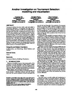
2) SymReg: SymReg is shown in Equation 30 and visualised in Figure 15. We generated 100 fitness cases by choosing 100 values for x from [-5,5] with equal steps. f (x) = exp(1 − x) × sin(2πx) + 50sin(x)

(30)

400

300

200

f(x)

Figures 8 and 13) and the selection probability distribution measure (see Figures 10 and 14). Overall, for the uniform and the random FRDs, the two tournament selections favour better-ranked individuals for all tournament sizes. For the reversed quadratic and the quadratic FRDs, the two skewed FRDs aggravate selection bias quite significantly. In particular, for the reversed quadratic FRD, there are more individuals of worse-ranked fitness that received selection preference. The GP search will still wander around without paying sufficient attention to the small number of outstanding individuals. Ideally, in this situation, a good selection schema should focus on the small number of good individuals to speed up evolution. For the random FRD, only slight fluctuations and differences can be found under very close inspection when comparing with the uniform FRD. Ideally, in this situation, a good selection scheme should be able to adjust the selection pressure distinguishably according to the changes in the fitness rank distribution. For instance, it should give a relatively higher selection preference to an individual in a fitness bag with smaller size in order to increase the chance of propagating this genetic material and a relatively lower selection preference to an individual in another fitness bag with larger size in order to reduce the chance of the same. For the quadratic FRD, the selection frequencies are strongly biased towards individuals with better ranks. The population diversity will be quickly lost, the convergence may speed up, and the GP search may be confined in local optima. Ideally, in this situation, a good selection scheme should slow down the convergence. Unfortunately, neither the no-replacement nor the round-replacement tournament selection can change parent selection pressure to meet the expectations. They are the same as standard tournament selection, being unable to know the dynamic requests, thus fail to tune parent selection pressure dynamically.

100

0

−100

−200 −5

Fig. 15.

0 x

5

The symbolic regression problem.

3) BinCla: BinCla involves determining whether examples represent a malignant or a benign breast cancer. The dataset is the Wisconsin Diagnostic Breast Cancer dataset chosen from the UCI Machine Learning repository [47]. BinCla consists of 569 data examples, where 357 are benign and 212 are malignant. It has 10 numeric measures (see Table I) computed from a digitised image of a fine needle aspirate of a breast mass and are designed to describe characteristics of the cell nuclei present in the image. The mean, standard error, and “worst” of these measures are computed, resulting in 30 features [47]. The whole original data set is split randomly and equally into a training data set, a validation data set, and a test data set with class labellings being evenly distributed across the three data sets for each individual GP run. B. function sets and terminal sets The function set used for EvePar consists of the standard Boolean operators { and, or, not } and if function. The if function takes three arguments and returns its second argument if the first argument is true, and otherwise returns its third argument. In order to increase the problem difficulty, we do not include the xor function in the function set. The function set used for SymReg includes the standard arithmetic binary operators { +, -, *, / } and unary operators { abs, sin, exp }. The / function returns zero if it is given invalid arguments. The function set used for BinCla includes the standard arithmetic binary operators { +, -, *, / }. We hypothesised that convergence might be quicker if using only the four arithmetic operators, and more functions might lead to better results. Therefore, the function set also includes unary operators { abs, sqrt, sin } and if function. The sqrt function automatically converts a negative argument to a positive one before operating on it. The if function takes three arguments and returns its second argument if the first argument is positive, and returns its third argument otherwise. The if function allows a program

16

to contain a different expression in different regions of the feature space, and allows discontinuous programs, rather than insisting on smooth functions. The terminal set for EvePar consists of n Boolean variables. The terminal set for SymReg and BinCla includes a single variable x and 30 terminals, respectively. Real valued constants in the range [-5.0, 5.0] are also included in the terminal sets for SymReg and BinCla. The probability mass assigned to the whole range of constants when constructing programs is set to 5%. TABLE I T EN FEATURES IN THE DATASET OF B IN C LA a b c d e

radius texture perimeter area smoothness

f g h i j

compactness concavity concave points symmetry fractal dimension

C. fitness function For even-n-parity problems, the standard fitness function counts the number of wrong outputs (misses) for the 2n combinations of n-bit strings and treats zero misses as the best raw fitness [1]. There is an issue with this fitness function: the worst program according to this fitness function is the one that has 2n misses. However, this program actually captures most of the structure of the problem and can be easily converted to a program of zero misses by adding a not function node to the root of the program. Therefore, programs with a very large number of misses are, in a sense, just as good as programs with very few misses. In this paper, we used a new fitness function for EvePar: m , if m < 2n−1 f itness = (31) n 2 − m , otherwise where m is the number of misses. The fitness function in SymReg is the root-mean-square (RMS) error of the outputs of a program relative to the expected outputs. Because neither class is weighted over the other, the fitness function for BinCla is the classification error rate on the training data set (the fraction of fitness cases that are incorrectly classified by a program as a proportion of the total number of fitness cases in the training data set). A program classifies the fitness case as benign if the output of the program is positive, and malignant otherwise. Note that class imbalance design in fitness function for BinCla is beyond the scope of this paper. All three problems have an ideal fitness of zero. D. genetic parameters and configuration The genetic parameters are the same for all three problems. The ramped half-and-half method is used to create new programs and the maximum depth of creation is four (counted from zero). To prevent code bloat, the maximum size of a program is set to 50 nodes during evolution based on some initial experimental results. The standard subtree crossover

and mutation operators are used [1]. The crossover rate, the mutation rate, and the copy rate are 85%, 10% and 5% respectively. The best individual in the current generation is explicitly copied into the next generation, ensuring that the population does not lose its previous best solution5 . A run is terminated when the number of generations reaches the predefined maximum of 101 (including the initial generation), or the problem has been solved (there is a program with a fitness of zero on the training data set), or the error rate on the validation set starts increasing (for BinCla). Three tournament sizes 2, 4, and 7 are used. Consequently, the population size is set to 504 in order to have zero remainder at the end of a round of tournaments in the round-replacement tournament selection. We ran experiments comparing three GP systems using the standard, the no-replacement, and the round-replacement tournament selections respectively for each of the three problems. In each experiment, we repeated the whole evolutionary process 500 times independently. In each pair of the 500 runs, an initial population is generated randomly and is provided to all GP systems in order to reduce the performance variance caused by different initial populations. E. Experimental results and analysis Table II compares the performances of the three GP systems. The measure for EvePar is the failure rate, measuring the fraction of runs that were not able to return the ideal solution. The best value is zero percent, meaning every run is successful. The measures for SymReg and BinCla are the averages of the RMS error and the classification error rate on test data over 500 runs respectively, thus the smaller the value, the better the performance. Note that the standard deviation is shown after the ± sign. TABLE II P ERFORMANCE COMPARISON BETWEEN THE NO - REPLACEMENT, ROUND - REPLACEMENT AND STANDARD TOURNAMENT SELECTION SCHEMES . Tournament Selection Scheme Size 2 standard 4 7 no2 replacement 4 7 round2 replacement 4 7

EvePar Failure (%) 100 80.6 82.4 100 80.6 82.5 99.6 79.4 77.6

SymReg RMS Error 48.2 ± 5.2 37.6 ± 8.3 40.9 ± 11.3 48.3 ± 5.2 37.6 ± 8.4 41.1 ± 11.2 47.4 ± 5.3 38.3 ± 8.0 40.6 ± 11.4

BinCla Test Error (%) 9.2 ± 2.9 8.7 ± 2.7 8.7 ± 2.7 9.2 ± 2.9 8.7 ± 2.7 8.7 ± 2.6 8.4 ± 2.7 8.6 ± 2.6 8.8 ± 2.7

The results demonstrate that the GP system using the noreplacement tournament selection has the almost identical performance as the GP system using standard tournament selection. The results confirm that for most common and reasonable tournament sizes and population sizes, the multisampled issue seldom occurs, and is not critical in GP. The results also show that the GP system using the roundreplacement tournament selection has some advantages over 5 This

is referred to as elitism [48].

17

the GP system using standard tournament selection. In order to provide statistically sound comparison results for the advantage of the round-replacement tournament selection, we calculated the confidence intervals at 95% and 99% levels (two-sided) for their differences in failure rates, in RMS errors, and in error rates for EvePar, SymReg and BinCla respectively. For EvePar, we used the formula q Pˆ1 − Pˆ2 ± Z Pˆ1 (1 − Pˆ1 )/500 + Pˆ2 (1 − Pˆ2 )/500 (32)

issue in a Genetic Algorithm using a tournament size of 2. Our experiments confirmed this in GP for some data sets and showed that the improvement was statistically significant, though not large. However, Sokolov and Whitley considered only tournament size 2. Our experiments included larger tournament sizes and showed that there was no statistically significant improvement for the larger tournament sizes in GP. Furthermore, the performance of larger tournament sizes with standard tournament selection was as good as or better than the performance of tournament size 2 with the round-replacement tournament selection. Therefore, there is no advantage in explicitly addressing the not-sampled issue. The analysis results show that although the not-sampled issue can be solved, overall the different selection behaviour provided by the round-replacement tournament selection alone appears to be unable to significantly improve a GP system for the given tasks. The not-sampled issue does not seriously affect the selection performance in standard tournament selection.

to calculate the confidence interval, where x¯ is the average difference over 500 values and s is the standard deviation. If zero is not included in the confidence interval, then the difference is statistically significant. Table III shows the confidence intervals only at the 95% level, since the statistical analysis results from the two levels are consistent. Significant differences (either better or worse) are shown in bold. According to the performance measures, the round-replacement tournament selection is better than the standard one when the confidence interval is less than zero.

IX. C ONCLUSIONS

where Pˆ1 is the failure rate using the round-replacement tournament selection, Pˆ2 is the failure rate using standard tournament selection, and Z is 1.96 for 95% confidence and 2.58 for 99% confidence. For SymReg and BinCla, we firstly calculated the difference of the measures between a pair of runs using the same initial population for each of the 500 pairs of runs, then used the formula s (33) x¯ ± Z √ 500

TABLE III C ONFIDENCE INTERVALS FOR DIFFERENCES IN PERFORMANCE BETWEEN THE ROUND - REPLACEMENT AND STANDARD TOURNAMENT SELECTION SCHEMES AT 95% LEVEL . Tournament size 2 4 7

EvePar (-0.95, 0.15) (-6.16, 3.76) (-9.75, 0.15)

SymReg (-1.48, -0.24) (-0.22, 1.57) (-1.47, 0.85)

BinCla (-1.05, -0.43) (-0.32, 0.24) (-0.25, 0.32)

From the table, for tournament size 2 and for SymReg and BinCla problems, the improvement of the round-replacement tournament selection is statistically significant. However, practically the differences are small. For tournament sizes 4 and 7, there are no statistically significant differences between the round-replacement and standard tournament selections. This is because only 1.8% and 0.09% of the population are not-sampled respectively in standard tournament selection (from Equation 8). There is little impact on the overall performance from the slight differences on the selection probability of the top-ranked programs. We also compared the best performance of the roundreplacement tournament selection with the best performance of the standard one for SymReg and BinCla; the differences were not statistically significant either. The results confirm that these extra sampled programs have limited contribution to the overall search performance. Sokolov and Whitley’s findings [49] suggested that performance could be improved by addressing the not-sampled

This paper clarified the impacts of multi-sampled and the not-sampled issues in standard tournament selection. It used the loss of program diversity, the selection frequency, and the selection probability distribution on four populations with different FRDs (fitness rank distributions) to simulate parent selection behaviours in the no-replacement and the roundreplacement tournament selections, which are the solutions to the multi-sampled and the not-sampled issues respectively. Furthermore, it provided experimental analyses of the noreplacement and the round-replacement tournament selections in three problem domains with different difficulties. The simulations and experimental analyses provided insight into the parent selection in tournament selection and the outcomes are as follows. The multi-sampled issue seldom occurs in standard tournament selection when common and realistic tournament sizes and population sizes are used. Therefore, although the sampling-without-replacement strategy in no-replacement tournament selection can solve the multi-sampled issue, there is no significantly different selection behaviour between noreplacement and standard tournament selection schemes. The simulation and experimental results justify the common use of the simple sampling-with-replacement scheme. The not-sampled issue mainly occurs when smaller tournament sizes are used in standard tournament selection. Our round-replacement tournament selection using an alternative sampling-without-replacement strategy can solve the issue without altering other aspects in standard tournament selection. The different selection behaviour in the round-replacement tournament selection compared with the standard one leads to better results only when tournament size 2 is used for some problems (those that need low parent selection pressure in order to find acceptable solutions). However, there is no significant performance improvement for relatively large and common tournament sizes such as 4 and 7. Solving the notsampled issue does not appear to significantly improve a GP system: the not-sampled issue in standard tournament selection

18

is not critical. Although this study is conducted in GP, the results are expected to be applicable to other EAs as we did not put any constraints on the representations of the individuals in the population. However further investigation needs to be carried out. Overall, different sampling replacement strategies have little impact on the parent selection pressure. Eliminating the multi-sampled issue and the not-sampled issues dose not significantly change the selection behaviour over standard tournament selection and cannot tune the selection pressure in dynamic evolution. In order to conduct effective parent selection in GP, further research should be emphasised on tuning parent selection pressure dynamically along evolution instead of developing alternative sampling replacement strategies. Since sometimes individuals can have almost, but not completely equal fitness values, selecting parents based purely on the fitness values of the individuals in the population may exaggerate selection pressure unnecessarily. In such cases, another interesting direction for future work is to consider fitness value intervals during selection. This work has also found that similar FRDs with different population sizes resulted in similar selection probability distributions. This indicate that population size itself might not significantly influence the selection pressure, but this needs to be further investigated in the future. ACKNOWLEDGEMENT We would like to thank Dr Peter Andreae for his comments, discussions and suggestions, and Dr Mark Johnston and Dr Ivy I-Ming Liu for their discussions on experiments. The experiments were carried out using the Genetic Progamming package Gouda. This work was also supported in part by the Marsden Fund council from the government funding (08-VUW-014), administrated by the Royal Society of New Zealand, and the University Research Fund (URF09-2399/85608) at Victoria University of Wellington for 2008–2009.

P ROOF

OF

A PPENDIX A E QUATIONS 20 AND 25 B EING E QUIVALENT

Proof: Equation 25 can be simplified to: Pj−1 Pk 1 (|Sj |−1)! i=1 |Si | n=1 n (n−1)!(|Sj |−1−n+1)! k−n P (Wj ) = N k Pj−1 Pk (|Sj |−1)! i=1 |Si | n=1 n!(|Sj |−n)! k−n = N k Pj−1 Pk |Sj |! 1 i=1 |Si | n=1 |Sj | n!(|Sj |−n)! k−n = N k

Pj−1 |Sj | i=1 |Si | n=1 n k−n = N |Sj | k Pn r s After applying the relation = m=0 m n−m r+s [50] (page 822), we can further simply the equan tion to Pj−1 P |Sj | |Sj | + j−1 |Si | i=1 |Si | i=1 − 0 k k = N |Sj | k Pj Pj−1 |Si | i=1 |Si | i=1 − k k = N |Sj | k Pk

which is the same as Equation 20.

R EFERENCES [1] J. R. Koza, Genetic Programming — On the Programming of Computers by Means of Natural Selection. Cambridge: MIT Press, 1992. [2] A. E. Eiben and J. E. Smith, Introduction to Evolutionary Computing. Springer, 2003. [3] P. Andreae, H. Xie, and M. Zhang, “Genetic programming for detecting rhythmic stress in spoken english,” International Journal of KnowledgeBased and Intelligent Engineering Systems. Special Issue on Genetic Programming., vol. 12, no. 1, pp. 15–28, 2008. [4] M. Brameier, W. Banzhaf, and F. Informatik, “A comparison of linear genetic programming and neural networks in medical data mining,” IEEE Transactions on Evolutionary Computation, vol. 5, pp. 17–26, 2001. [Online]. Available: http://citeseerx.ist.psu.edu/viewdoc/ summary?doi=10.1.1.41.208 [5] L. B. de Sa and A. Mesquita, “Evolutionary synthesis of low-sensitivity equalizers using adjacency matrix representation,” in Proceedings of the 10th annual conference on Genetic and evolutionary computation, M. Keijzer, G. Antoniol, C. B. Congdon, K. Deb, B. Doerr, N. Hansen, J. H. Holmes, G. S. Hornby, D. Howard, J. Kennedy, S. Kumar, F. G. Lobo, J. F. Miller, J. Moore, F. Neumann, M. Pelikan, J. Pollack, K. Sastry, K. Stanley, A. Stoica, E.-G. Talbi, and I. Wegener, Eds. Atlanta, GA, USA: ACM, 12-16 Jul. 2008, pp. 1283–1290. [6] J. R. Koza, F. H. B. III, D. Andre, and M. A. Keane, Genetic Programming III: Darwinian Invention and Problem Solving, 1st ed. Morgan Kaufmann, May 1999. [7] R. L. Popp, D. J. Montana, R. R. Gassner, G. Vidaver, and S. Iyer, “Automated hardware design using genetic programming, VHDL, and FPGAs,” in IEEE International Conference on Systems, Man, and Cybernetics, vol. 3. San Diego, CA USA: IEEE, 11-14 Oct. 1998, pp. 2184–2189. [8] D. Agnelli, A. Bollini, and L. Lombardi, “Image classification: an evolutionary approach,” Pattern Recognition Letters, vol. 23, no. 1-3, pp. 303– 309, 2002. [Online]. Available: http://www.sciencedirect.com/science/ article/B6V15-443K10X-6/1/7af8206767ca79f9898fec720a84c656 [9] A. Akyol, Y. Yaslan, and O. K. Erol, “A genetic programming classifier design approach for cell images,” in Proceedings of the 9th European Conference on Symbolic and Quantitative Approaches to Reasoning with Uncertainty, ECSQARU, ser. Lecture Notes in Computer Science, K. Mellouli, Ed., vol. 4724. Hammamet, Tunisia: Springer, Oct. 31 Nov. 2 2007, pp. 878–888. [10] R. Vanyi, “Practical evaluation of efficient fitness functions for binary images,” in Applications of Evolutionary Computing, EvoWorkshops2005: EvoBIO, EvoCOMNET, EvoHOT, EvoIASP, EvoMUSART, EvoSTOC, ser. LNCS, F. Rothlauf and et al, Eds., vol. 3449. Lausanne, Switzerland: Springer, 30 Mar.-1 Apr. 2005, pp. 310–324. [11] F. Castillo, A. Kordon, J. Sweeney, and W. Zirk, “Using genetic programming in industrial statistical model building,” in Genetic Programming Theory and Practice II, U.-M. O’Reilly and et al, Eds. Springer, 2006, ch. 3, pp. 31–48.

19

[12] G. Smits, A. Kordon, K. Vladislavleva, E. Jordaan, and M. Kotanchek, “Variable selection in industrial datasets using pareto genetic programming,” in Genetic Programming Theory and Practice III, ser. Genetic Programming, T. Yu, R. L. Riolo, and B. Worzel, Eds. Ann Arbor: Springer, 12-14 May 2005, vol. 9, ch. 6, pp. 79–92. [13] M. D. Schmidt and H. Lipson, “Learning noise,” in Proceedings of the 9th annual conference on Genetic and evolutionary computation, D. Thierens, H.-G. Beyer, J. Bongard, J. Branke, J. A. Clark, D. Cliff, C. B. Congdon, K. Deb, B. Doerr, T. Kovacs, S. Kumar, J. F. Miller, J. Moore, F. Neumann, M. Pelikan, R. Poli, K. Sastry, K. O. Stanley, T. Stutzle, R. A. Watson, and I. Wegener, Eds., vol. 2. London: ACM Press, 7-11 Jul. 2007, pp. 1680–1685. [14] W.-C. Lee, “Genetic programming decision tree for bankruptcy prediction,” in Proceedings of the 2006 Joint Conference on Information Sciences, JCIS 2006. Kaohsiung, Taiwan, ROC: Atlantis Press, Oct. 8-11 2006. [Online]. Available: http://www.atlantis-press. com/php/download paper?id=8 [15] J. Li and E. P. K. Tsang, “Reducing failures in investment recommendations using genetic programming,” in Computing in Economics and Finance, Universitat Pompeu Fabra, Barcelona, Spain, 6-8 Jul. 2000. [16] W. Zhang, Z. ming Wu, and G. ke Yang, “Genetic programming-based chaotic time series modeling,” Journal of Zhejiang University Science, vol. 5, no. 11, pp. 1432–1439, 2004. [17] J.-H. Hong and S.-B. Cho, “Lymphoma cancer classification using genetic programming with snr features,” in Proceedings of 7th EuroGP Conference, 2004, pp. 78–88. [Online]. Available: http: //www.springerlink.com/content/w51g1mbxmxtbg7pd [18] M. Zhang, V. Ciesielski, and P. Andreae, “A domain independent window-approach to multiclass object detection using genetic programming,” EURASIP Journal on Applied Signal Processing, vol. 2003, no. 8, pp. 841–859, 2003. [19] M. Zhang, X. Gao, and W. Lou, “Gp for object classification: Brood size in brood recombination crossover,” in The 19th Australian Joint Conference on Artificial Intelligence, ser. LNAI, vol. 4303. Springer, 2006, pp. 274–284. [20] J. H. Holland, Adaptation in Natural and Artificial Systems. Ann Arbor: University of Michigan Press, 1975. [21] J. J. Grefenstette and J. E. Baker, “How genetic algorithms work: A critical look at implicit parallelism,” in Proceedings of the 3rd International Conference on Genetic Algorithms, J. D. Schaffer, Ed. Morgan Kaufmann Publishers, 1989, pp. 20–27. [22] A. Brindle, “Genetic algorithms for function optimisation,” Ph.D. dissertation, Department of Computing Science, University of Alberta, 1981. [23] J. R. Koza, M. A. Keane, M. J. Streeter, W. Mydlowec, J. Yu, and G. Lanza, Genetic programming IV: Routine Human-Competitive Machine Intelligence. Kluwer Academic, 2003. [24] T. B¨ ack, “Selective pressure in evolutionary algorithms: A characterization of selection mechanisms,” in Proceedings of the First IEEE Conference on Evolutionary Computation., 1994, pp. 57–62. [25] T. Blickle and L. Thiele, “A mathematical analysis of tournament selection,” in Proceedings of the Sixth International Conference on Genetic Algorithms, 1995, pp. 9–16. [26] ——, “A comparison of selection schemes used in evolutionary algorithms,” Evolutionary Computation, vol. 4, no. 4, pp. 361–394, 1997. [27] J. Branke, H. C. Andersen, and H. Schmeck, “Global selection methods for SIMD computers,” in Proceedings of the AISB96 Workshop on Evolutionary Computing, 1996, pp. 6–17. [28] D. E. Goldberg and K. Deb, “A comparative analysis of selection schemes used in genetic algorithms,” Foundations of Genetic Algorithms, pp. 69–93, 1991. [29] B. L. Miller and D. E. Goldberg, “Genetic algorithms, tournament selection, and the effects of noise,” University of Illinois at UrbanaChampaign, Tech. Rep. 95006, July 1995. [30] ——, “Genetic algorithms, selection schemes, and the varying effects of noise,” Evolutionary Computation, vol. 4, no. 2, pp. 113–131, 1996. [31] T. Motoki, “Calculating the expected loss of diversity of selection schemes,” Evolutionary Computation, vol. 10, no. 4, pp. 397–422, 2002. [32] R. Poli and W. B. Langdon, “Backward-chaining evolutionary algorithms,” Artificial Intelligence, vol. 170, no. 11, pp. 953–982, 2006. [33] H. Xie, M. Zhang, and P. Andreae, “Population clustering in genetic programming,” in Proceedings of the 9th European Conference, EuroGP 2006, ser. LNCS, vol. 3905. Springer, 2006, pp. 190–201. [34] ——, “Automatic selection pressure control in genetic programming,” in Proceedings of the sixth International conference on Intelligent Systems Design and Applications. IEEE Computer Society Press, 2006, pp. 435–440.

[35] M. Affenzeller, S. Wagner, and S. Winkler, “GA-selection revisited from an ES-driven point of view,” in Artificial Intelligence and Knowledge Engineering Applications: A Bioinspired Approach, ser. Lecture Notes in Computer Science. Springer, 2005, vol. 3562, pp. 262–271. [36] H. Xie, M. Zhang, and P. Andreae, “An analysis of constructive crossover and selection pressure in genetic programming,” in Proceedings of Genetic and Evolutionary Computation Conference, 2007, pp. 1739– 1746. [37] S. Winkler, M. Affenzeller, and S. Wagner, “Offspring selection and its effects on genetic propagation in genetic programming based system identification,” Cybernetics and Systems, vol. 2, pp. 549–554, 2008. [38] ISCID, “Iscid encyclopaedia of science and philosophy,” 2006. [Online]. Available: http://www.iscid.org/encyclopedia/Selection Pressure [39] G. Dark, “On-line medical dictionary,” 2005. [Online]. Available: http://cancerweb.ncl.ac.uk/cgi-bin/omd [40] FAO, “Glossary of biotechnology and genetic engineering,” 2008. [Online]. Available: http://www.fao.org/DOCREP/003/X3910E/ X3910E22.htm [41] V. Ciesielski and D. Mawhinney, “Prevention of early convergence in genetic programming by replacement of similar programs,” in Proceedings of the 2002 Congress on Evolutionary Computation. IEEE Press, 2002, pp. 67–72. [42] M. Bulmer, The Mathematical Theory of Quantitative Genetics. Oxford, UK: Oxford University Press, 1980. [43] H. Muhlenbein and D. Schlierkamp-Voosen, “Predictive models for the breeder genetic algorithm, I: continuous parameter optimization,” Evolutionary Computation, vol. 1, no. 1, pp. 25–49, 1993. [44] E. Popovici and K. D. Jong, “Understanding EA dynamics via population fitness distributions,” in Proceedings of the Genetic and Evolutionary Computation Conference 2003, 2003, pp. 1604–1605. [45] H. Xie, M. Zhang, and P. Andreae, “Another investigation on tournament selection: modelling and visualisation,” in Proceedings of Genetic and Evolutionary Computation Conference, 2007, pp. 1468–1475. [46] S. M. Gustafson, “An analysis of diversity in genetic programming,” Ph.D. dissertation, University of Nottingham, 2004. [47] D. Newman, S. Hettich, C. Blake, and C. Merz, “UCI repository of machine learning databases,” 1998. [Online]. Available: http: //archive.ics.uci.edu/ml [48] R. Poli, N. F. McPhee, and L. Vanneschi, “Elitism reduces bloat in genetic programming,” in Proceedings of the 10th annual conference on Genetic and evolutionary computation. ACM Press, 2008, pp. 1343– 1344. [49] A. Sokolov and D. Whitley, “Unbiased tournament selection,” in Proceedings of Genetic and Evolutionary Computation Conference. ACM Press, 2005, pp. 1131–1138. [50] M. Abramowitz and I. A. Stegun, Eds., Handbook of Mathematical Functions. New York: Dover, 1965.

Sampling Issues of Tournament Selection in Genetic Programming

Sampling Issues of Tournament Selection in Genetic Programming

Suggest Documents

Open issues in genetic programming - Semantic Scholar

Open issues in genetic programming - Semantic Scholar

Model Selection in Genetic Programming

Model Selection in Genetic Programming

Discriminant Feature Selection by Genetic Programming - CiteSeerX

Genetic Programming with User-Driven Selection ... - CiteSeerX

Tuning Selection Pressure in Tournament Selection - School of ...

Tournament Selection, Iterated Coupon-Collection

Tournament Selection' Stable Fitness Pressure in ...

Genetic programming for model selection of TSK ... - Semantic Scholar

Selection and Evaluation of Test Data Based on Genetic Programming

GENETIC PROGRAMMING

Genetic Programming

Genetic Programming

Genetic Programming

Genetic Programming –

Quality Issues in Water Sampling, Sample Pre

The Sampling Issues in Quantitative Research - Eric

Sampling in epidemiological research: issues ... - BJPsych Bulletin

Mixed size tournament selection - Springer Link

Another Investigation on Tournament Selection: modelling and ...

Constraint Handling Using Tournament Selection ... - CiteSeerX

FINE-GRAINED TOURNAMENT SELECTION ... - Semantic Scholar

Tournament Selection for Browsing Temporal ... - Infoscience - EPFL