MARINE ECOLOGY PROGRESS SERIES Mar Ecol Prog Ser
Published April 18
Sampling patchy distributions: comparison of sampling designs in rocky intertidal habitats A. Whitman Miller, Richard F. Ambrose* Environmental Science and Engineering Program. Box 951772. University of California, Los Angeles. California 90095-1772, USA
ABSTRACT: Any attempt to assess species abundances must employ a sampling design that balances collection of accurate information for many species with a reasonable sampling effort. To assess the accuracy of commonly used withln-site sampling designs for sessile species, we gathered cover data at 2 rocky intertidal locations in Southern California using a high-density point-contact method that maintained the spatial relationships among all points. Different sampling approaches were compared using simulated sampling. Different sampling units (single points, line transects, and quadrats) were modeled at high and low sampling efforts. Sampling units were either distnbuted randomly or with stratified random methods. Sampling accuracy was assessed by comparing cover and species richness estlrnated by the sampling simulations to the actual field data. Randomly placed single point-contacts provlded the best estimates of cover but are usually not logistically feasible in the rocky intertidal, so ecologists typically use quadrats or line transects. With quadrats, some form of stratified random sampling usually gave estimates that were closer to known values than slmple random placement. In nearly all stratified cases, optimum allocation of sample units, where quadrats are allocated among strata according to the amount of variability within each stratum, yielded the most accurate estimates. With 1 exception, line transects placed perpendicular to the elevational contours ('vertical transects') approached or exceeded the accuracy of the best stratified quadrat efforts. The estimates for rare species were consistently poor since sampling units often missed such species altogether, suggesting a systematic blas. Species richness was substantially underestimated by all sampllng approaches tested, whereas these same approaches accurately estimated diversity (H').These results illustrate the difficulty of obtaining accurate cover estimates in rocky intertidal communities.
KEY WORDS: Sampling deslgn . Monitonng . Quadrats . Transects . Stratified random sampling Rocky intertidal . Southern California
INTRODUCTION Species are rarely dispersed uniformly in nature (Oosting 1956, Pielou 1977, Whittaker & Levin 1977, Kolasa & Pickett 1991). Instead, spatial heterogeneity is the norm, and ecological field studies and environmental monitoring programs must be designed accordingly (Green 1979, Hartnoll & Hawkins 1980, Hurlbert 1984, Andrew & Mapstone 1987, Eberhardt & Thomas 1991, Underwood 1992). Although the issue of sampling patchily distributed populations cuts across all habitats and taxa, plant ecologists in particular have tried to understand the best methods for sampling 'Corresponding author. E-mail:
[email protected] O Inter-Research 2000 Resale of full article not permitted
spatially variable communities (Raunkiaer 1918, Gleason 1920, Oosting 1956, Greig-Smith 1983). In recent years, issues of sampling scale and spatial heterogeneity have become central to terrestrial and marine ecologists who study community structure and function (Andrew & Mapstone 1987, Foster 1990, Menge & Olson 1990, Reed et al. 1993, Edmunds & Bruno 1996). The rocky intertidal has exceptionally high levels of spatial variability and the difficulties associated with measuring patterns of abundance in these habitats are well known (Hartnoll&Hawkins 1980, M. N. Dethier & L. M. Tear unpubl.). Recent work has focused on the accuracy of different methods for estimating the cover of sessile organisms within a small area (i.e., quadrat) on rocky intertidal benches, such as comparing visual
Mar Ecol Prog Ser 196: 1-14, 2000
estimates and point-contact methods (Foster et al. 1991, Meese & Tomich 1992, Whorff & Griffing 1992, Dethier et al. 1993, Rivas 1997). There have been few studies on how different types of sampling units (e.g., transects or quadrats) and sampling designs (e.g.,random or stratified random) affect the estimates of cover over a larger region (Hartnoll & Hawkins 1980). The development of effective sampling programs in the intertidal and other spatially heterogeneous habitats depends on how well we can expect to estimate species abundances and what sampling designs best balance sampling effort with sampling accuracy. In this paper, we use a combination of detailed data on actual species occurrences and computer simulations to assess the accuracy of different sampling designs. Data from 2 rocky intertidal sites were repeatedly resampled, with the sampling simulation results compared to the field data to determine which design was most likely to yield estimates matching the field data. Estimates of species cover, species richness, and biological diversity were compared when sampling unit type, number, and dispersion were systematically varied. The results provide guidance about the most effective approach for sampling a heterogeneous habitat such as rocky intertidal benches, but they also high~iy~ estimates of light .he&C 1 1 ~ ~ 1oft y~ i ~ d i i C i accurate abundance with the limited resources typically available for monitoring efforts. Repeated sampling has been used previously to understand the efficacy of various sampling techniques in heterogeneous habitats. Before the advent of personal computers, Bauer (1943) compared the accuracy of quadrat and transect sampling techniques by manually measuring cover in artificial 'plant communities' in the laboratory (randomly placed colored cardboard disks of various abundances and sizes). Subsequent empirical field studies of a fully mapped segment of Southern California chaparral supported his prediction that lineintercept methods provided superior accuracy to quadrat methods in this plant community. Bauer had limited ability to resample and his artificial plant population~lacked the true spatial variability encountered in nature. Nonetheless, we share his goal of reducing sampling error in a spatially heterogeneous setting by understanding the consequences of different sampling approaches. Several other workers have more recently used computer simulations to evaluate different sampling issues (Wiebe 1971, Kinzie & Snider 1978, Hellmann & Fowler 1999).Some computer-based sampling studies relying on simulated data have focused on sampling methodology rather than sampling design (Kinzie & Snider 1978, Dethier et al. 1993, Rivas 1997), and thus were concerned only with the distribution of organisms on the scale of an individual quadrat. Andrew & Mapstone (1987) warn that extrapolations
from computer to nature should be treated cautiously unless the simulations are constructed on a sound knowledge about the distribution and behavior of the organisms in natural conditions. For questions concerning sampling design over an entire study area, the data set should reflect the actual spatial structure of the community. We have ensured that our simulations reflect natural patterns by basing them on intensive sampling of actual rocky intertidal conlrnunities. Using computers to simulate sampling has advantages over actual resampling. Simulated sampling offers substantial time savings and increased flexibility. Because repeating actual sampling procedures is so time-consuming, the few studies that have attempted this have been limited to only a few replicates (e.g.,Foster et al. 1991, Dethier et al. 1993, Arnbrose et al. 1995, Rivas 1997). The increased efficiency also allows the comparison of more alternative approaches. Simulated sampling also ensures constancy of the data set. A computer-based reference data set is fixed and therefore any differences in results are true differences. In contrast, placement or alignment errors of the measuring device in the field can introduce significant changes to the domain being sampled (Ellison 1942, Ambrose et al. 1995).In addition, the period needed for extensive intertidal field sampling wou!d bz prctracte:! because sampling time is limited by appropriate tides, leading to a significant risk of actual changes in the species occurrences. In contrast, the reference data set for computer-based resampling is constant.
METHODS
Terminology. Accuracy is the closeness of a measured value to its true value; precision is the closeness of repeated measurements of the same quantity (Sokal & Rohlf 1981). Bias refers to a systematic displacement from the true value. Unless there is a bias in measurements, precision will lead to accuracy. Thus, an accurate sampling protocol is one that produces an unbiased sample with high precision. We have focused on assessing the accuracy of different protocols. Study sites. The 2 study sites chosen were typical of Southern California rocky bench habitats. We chose areas in the mid- to upper intertidal zone with roughly similar elevational gradients and without sharp topographical features such as high pinnacles or deep surge channels. The specific study plots were selected because they contained a variety of species (e.g., mussels, barnacles, and algae) and were typical of the surrounding bench habitat. The White's Point study site is part of a volcanlc rocky bench located on the Palos Verdes Peninsula, Los Angeles County, California (33"42' 55" N, 118" 18' 58" W).
Miller & Ambrose: Sam~plingpatchy distributions
A 10 m X 10 m square study area dominated by California mussels Mytilus californianus, barnacles Chthamalus spp., including C. fissus and C. dalli, and Balanus glandula, and the red alga Endocladia muricata was measured and marked at all corners with marine epoxy. The study area is not directly exposed to breaking waves; instead, waves and surge break over the top of the promontory and flow down across the area. A second site at Shaw's Cove, Orange County, California (33"33' 15" N , 117 " 47' 59" W), approximately 65 km south of White's Point, was chosen for comparative purposes, since agreement between sites would suggest greater generalizability about sampling efficacy in Southern California rocky intertidal bench habitats. The area sampled at Shaw's Cove measured 5 m X 5 m and was dominated by California mussels Endocladia muricata, Chtharnalus spp., and non-coralline crusts. This study area has a rugose surface with cracks that maintain some standing water at low tide. Cover measurement and reference data set production. For estimating cover of sessile invertebrates and algae, we gathered point-contact data at 10 cm intervals in a 1 m X 1 m grid on the bench surface. Grids were aligned contiguously and covered the entire area of each study site, yielding 10000 sample points at White's Point and 2500 points at Shaw's Cove. To locate the point contacts, a 1.2 m X 1.2 m alurninum quadrat was constructed and strung with nylon-coated steel cable at 10 cm intervals, creating one hundred 10 cm X 10 cm square cells. Point contact locations were determined with a laser pointer (654 nm wavelength, 5 mW power output) mounted in a block that fit snugly among the wires surrounding a grid cell. When the laser block was positioned, the laser beam was centered and projected downward, normal to the grid surface. The laser cast a small red spot (approximately 2 mm diameter at 1 m height) on the bench surface, highlighting the organism to be counted. The laser block was moved sequentially from cell to cell to generate an array of data points. Besides providing unambiguous point-contact sampling without parallax problems, this quadrat design allowed the sampler to kneel beneath the frame for easier species identification. Using a laser beam instead of a sampling rod (as is frequently used with this method; Foster et al. 1991) also allowed precise sampling at distances of more than 1 m below the quadrat, a condition commonly encountered when sampling among surge channels, deep tide pools, steep drop-offs, and other topographical features of the intertidal. Finally, the laser system provided a simple way to align the quadrat within the study site. By placing a laser at each of the 4 quadrat corner cells and marking the contact points on the substrate below, the quadrat could be systematically moved around the site.
3
At White's Point and Shaw's Cove, layering of organisms was relatively infrequent. When layering was encountered, only the organism attached to the substrate was recorded. Taxonomic identification was generally done to species level, except for taxa such as encrusting algae that could not be easily identified in the field. Species contact data were gathered in sequence within each quadrat. Knowing the quadrat location and preserving the order of data collection allowed us to maintain the spatial relationship of each data point relative to all others. Species data files were imported into IDRISI (Clark University), a raster-based geographic information system, and a map describing the location of each species was generated. Sampling at White's Point was completed between December 1995 and February 1996; sampling at Shaw's Cove was completed between March and April 1996. Simulated sampling. Cover (%) was calculated for all specles based on all point-contacts at a site. In addition to cover, we calculated species richness (the number of species) and species diversity. Diversity of biological cover (bare rock cover not included) was calculated using the Shannon-Wiener index (H')(Shannon & Weaver 1949). The reference data sets were subsampled using a computer program that allowed us to locate 'virtual' transects, quadrats and single point-contacts over each study site. The sampling unit type, number, dispersion, and number of times a data set was to be resampled could be specified. In addition, sampling units could be allocated according to specified stratification criteria. The results from resampling queries were compared with actual cover values from the complete reference data sets. Six of the most abundant taxa at both sites were included in a series of sampling protocol comparisons. For each species, 2 sampling unit types were investigated, line transects and 0.5 m X 0.5 m quadrats, chosen because of their common usage in rocky intertidal studies. For each simulation, multiple transects or quadrats comprised a sample. Point-contacts were recorded every 10 cm along a line for transects and at the same interval in an array pattern for quadrats. To simulate simple random point sampling, individual randomly located points were sampled using the White's Point data set. Sampling effort was either 300 or 1000 point-contacts (3 and 10% of total points) at White's Point and 150 or 250 point-contacts (6 and 10 % of total points) at Shaw's Cove. The sampling efforts correspond to 3 and 10 'virtual' transects (i.e.,transects pulled from the computer database) at White's Point and 3 and 5 transects at Shaw's Cove. On average, transects were placed every 3.3 or 1 m at White's Point and every 2.5 or 1 m at Shaw's
Mar Ecol Prog Ser 196: 1-14, 2000
Cove. Transects were run either parallel to the site's primary slope (i.e., from the upper intertidal to the lower intertidal: 'vertical transects') or perpendicular to this slope ('horizontal transects'). For all transect protocols, transects were distributed randomly over the entire site. The number of quadrats used for subsampling contained similar numbers of point-contacts as corresponding transect efforts (12 and 40 quadrats at White's Point, 6 and 10 quadrats at Shaw's Cove). Quadrats were chosen from the set of contiguous, nonoverlapping 0.5 m X 0.5 m quadrats covering the entire site. Precluding quadrat overlap and not allowing quadrats to fall partly off the study site avoided artifactual sampling biases produced by edge effects. Although this model design does not incorporate every possible quadrat location, it does reflect the type of non-overlapping quadrat placement that would be used in the field. When sampled randomly, each potential quadrat location had an equal likelihood of selection. Since organisms are not distributed evenly throughout the intertidal, the variability associated with their cover can be markedly different over a small area. A varying spatial pattern within a study area can result in an overdii ~eciuctioniil sainpiing precision (Andrew & Mapstone 1987, Hayne 1987). Stratification, the subdivision of an area into more homogeneous areas with samples allocated among these subdivided areas, can be used to reduce the influence of spatial variability. The effect of stratifying quadrat location was evaluated using the White's Point data set. The study area was divided into 4 strata, with 3 main strata based on elevation and the uppermost stratum further subdivided into 2 sections based on whether or not the area fell within the splash shadow created by a large boulder. Once stratification is imposed, a decision must still be made about how to allocate sampling units among the strata. Two methods were employed in this study. The first method simply allocated sampling units in proportion to area, regardless of any inter-stratum differences in spatial variability ('Proportional Stratified Sampling' in Andrew & Mapstone 1987). For example, if 100 sampling units were to be allocated to 3 strata covering 20, 50, and 30% of the site, then 20, 50, and 30 quadrats would be allocated, respectively. The second method allocated sampling units on the basis of per-quadrat spatial variance of each species within each stratum, with more samples allocated to areas with higher variances, in a so-called 'optimum' allocation scheme (Cochran 1977; 'Stratified Sampling with Optimal Allocation' in Andrew & Mapstone 1987). Spatial variance estimates can be calculated using the species cover within each of the strata:
vij = d[(coverij)X (l-cover,,)], where v. denotes the spatial variance of the ith species in the jth stratum. For each species, 4 variances were calculated, 1 for each stratum. These variances were then normalized by dividing each by the sum of all 4. For example, the normalized variance for species 1 in stratum 1, V,,, was calculated as vI1/(vII+ v12+ V13 + v14)The sample size for species 1 in stratum 1 was then calculated by multiplying the total number of sample quadrats to be allocated across the site, either 40 or 12, by V,,. This procedure increases the precision of cover estimates by sampling more intensely in strata with more variable populations than in strata with relatively homogeneous populations. In an actual field situation, spatial variation would be estimated with the above equation and sampling units allocated accordingly. Since cover values were known for all species in each stratum at White's Point, these actual values were used to optirnize quadrat allocation, which may have slightly enhanced the effects of optimum quadrat allocation over what might be realized in the field. For both allocation methods, quadrats were positioned randomly within each stratum. Resampling. To understand the range of results typical of each sampling protocol, data sets were sampled repeatedly using a Monte Csrlo resampling rfie:hod. For example, to assess how well 3 randomly placed sampling units predicted the true cover of a particular taxon, we used a computer subsampling routine to perform the following tasks: (1) For each iteration, randomly locate the 3 sample units across the study site. (2) Compare the estimated cover (or species diversity) to the true cover (or species diversity) based on the full data set. A normalized deviation from true cover (A) was calculated by subtracting the true cover value from the sample value (i.e., the result of each iteration) and dividing this difference by the true cover: A = (sample-true)/true. By normalizing cover estimates, taxa with different actual cover values can be compared to one another on identical scales. (3)Repeat this process 5000 times (or the maximum possible number of unique combinations of randomly placed sampling units). Five thousand iterations give an adequate estimate of the full range of variability in the data set (Manly 1992, unpubl. data). Thus, for each protocol tested, a frequency distribution of 5000 A values was generated. Since field surveys usually consist of just 1 sampling effort per location per time, analogous to a single iteration, the A frequency distribution can be used to indicate how close estimates from an individual sampling effort are likely to be to the actual field value. If most of the iterations are close to the true value, then a single field survey is likely to provide a good estimate of the true value. Box plots provide a visual and quantitative
5
Mdler & Ambrose: Sampling patchy distributions
(A)
1400
Endocladia - 3 vertical transects 5000 Sarnoles - (True Cover = 0.0961)
1000 -
i 3 C a,
3 0-
1400 lIoo
1I
Chthamalus - 12 auadrats. 5000 Sarn~les (True Cover = 0408)
1000
800 -
,11111 800
600 -
LL
400 -
0
l
k
1.
400
200
,
,
Cover Estimates
0
,
,
,
Cover Estimates
500 Normalized Deviation from True Cover Value
Normalized Deviation from True Cover Value
Delta = (Sample - Tnre)TTrue
Delta = (Sample - True)/True
(C) Normalized Deviation from True Cover Value
Delta = (Sample - True)TTrue
1 I
Normalized Deviation from True Cover Value
Delta = (Sample - True)TTrue
Fig. 1. Graphical summary of Monte Carlo sampling simulations and comparisons to true values. Simulations of 2 different sampling designs are Illustrated with 2 species. (A) Frequency distributions of cover estimates generated by Monte Carlo simulations; units = fraction of cover. (B) A distribution of the estimates shown in A. (C) Box plot of A distribution. The dashed vertical line represents mean; solid vertical line represents median; box outlines the interquartile region; whiskers (lines extending from the box) indicate 10th and 90th percentiles, and circles mark the 5th and 95th percentiles
summary of A distributions for easy comparison among sampling protocols. The steps in this process are summarized in Fig. 1. Cover estimates generated by Monte Carlo simulations can be depicted as frequency distributions (Fig. 1A). The simulation results can also be presented as normalized
deviations from the true cover, either as A distributions (Fig. 1B) or box plots (Fig. 1C). Accuracy of different sampling protocols and taxa can be compared by examining interquartile ranges in box plots. Box plots can be helpful for detecting differences in sampling precision and bias that are not readily apparent with cover fre-
Mar Ecol Prog Ser 196: 1-14,2000
6
quency distributions. For example, the box plots show that most estimates of Endocladia muricata cover were closer to the true cover value than the estimates for Chthamalus spp. cover (Fig. lC), in spite of apparently similar cover frequency distributions (Fig. 1A).
RESULTS
tar, were encountered at Shaw's Cove. Twelve species accounted for 99% of the biological cover; in addition to the common species at White's Point, encrusting algae (coralline and Ralfsiaceae) and Pelvetia fastigiata were also common (Table 1, Fig. 3). M, californianus was much more common at Shaw's Cove. Many more rare species were encountered at White's Point. Bare rock occupied the most area at both sites.
Field data
mrl ,
Estimates of cover from sampling simulations
Thirty taxa, plus bare rock, were encountered at White's Point. Of these, 14 species accounted for over 99% of the cover there; barnacles Balanus glandula and Chthamalus spp., Endocladia muncata and Mytilus californianus were the most common species (Table 1, Fig. 2). Fifteen taxa, in addition to rock and
-..
..m
.-L 1 ; : ; a
, --,.
.' '*-$pi $ a:
:-
l^,
? .:
. r
.
:.,
'.I
,*? ?> :
- .. ., : - - -:;.&-;:-:. : > )$K-...2. .. v.. -- ,1 . . :-; { .. :- .,,*. .- ?-8.:.r.-p , . -. .-. .I . --_. . .. ,"..
-. I..
.
Endociadia
m
. . ' X
.,+--l
--
.
m
?.:D .
,
-5:
No systematic sampling bias, as indicated in box plots by sample distribution means that deviate strongly from A = 0, was found for any of the sampling protocols used to estimate cover of the common species at White's Point or Shaw's Cove (Figs. 4 & 5).
'..