Sampling the Repairs of Functional Dependency Violations under Hard Constraints George Beskales
Ihab F. Ilyas
Lukasz Golab
University of Waterloo
University of Waterloo
AT&T Labs - Research
[email protected]
[email protected]
[email protected]
ABSTRACT Violations of functional dependencies (FDs) are common in practice, often arising in the context of data integration or Web data extraction. Resolving these violations is known to be challenging for a variety of reasons, one of them being the exponential number of possible “repairs”. Previous work has tackled this problem either by producing a single repair that is (nearly) optimal with respect to some metric, or by computing consistent answers to selected classes of queries without explicitly generating the repairs. In this paper, we propose a novel data cleaning approach that is not limited to finding a single repair or to a particular class of queries, namely, sampling from the space of possible repairs. We give several motivating scenarios where sampling from the space of FD repairs is desirable, propose a new class of useful repairs, and present an algorithm that randomly samples from this space. We also show how to restrict the space of generated repairs based on user-defined hard constraints that define an immutable trusted subset of the input relation, and we experimentally evaluate our algorithm against previous approaches. While this paper focuses on repairing FDs, we envision the proposed sampling approach to be applicable to other integrity constraints with large repair spaces.
1.
INTRODUCTION
Functional dependencies (FDs) can be thought of as integrity constraints that encode data semantics. In that sense, violations of FDs indicate deviations from the expected semantics, possibly caused by data quality problems. In practice, FDs tend to break after integrating heterogeneous data or extracting data from the Web. Even in a traditional DBMS, unknown FDs may be hidden in a complex evolving schema, or the database administrator may choose not to enforce some FDs for various reasons. For example, Figure 1 shows a database instance and a set of FDs, some of which are violated (e.g., tuples t2 and t3 violate ZIP→City, tuples t2 and t3 violate Name→ SSN,City, and tuples t1 and t4 violate ZIP → State,City). There is often a very large number of ways to modify a table so that it satisfies all the required FDs. One way is to delete the offending tuples (ideally, delete the fewest possible such tuples) such Permission to make digital or hard copies of all or part of this work for personal or classroom use is granted without fee provided that copies are not made or distributed for profit or commercial advantage and that copies bear this notice and the full citation on the first page. To copy otherwise, to republish, to post on servers or to redistribute to lists, requires prior specific permission and/or a fee. Articles from this volume were presented at The 36th International Conference on Very Large Data Bases, September 13-17, 2010, Singapore. Proceedings of the VLDB Endowment, Vol. 3, No. 1 Copyright 2010 VLDB Endowment 2150-8097/10/09... $ 10.00.
Input Instance SSN
Name
State
ZIP
t1 72163 John Smith Chicago
City
IL
90101
t2 87991 Mark Green
CA
90065
LA Los
t3 87891 Mark Green Angeles t4 23212 Mary Clarke LA
CA
90065
CA
90101
Functional Dependencies:
SSN → Name, City, State, ZIP Name → SSN, City, State, ZIP ZIP → State, City
Repair 1 SSN
Name
City
Repair 2 State ZIP
SSN
Name
City
State ZIP
72163 John Smith
LA
CA
90101
72163 John Smith Chicago
IL
?
87991 Mark Green
LA
CA
90065
87891 Mark Green
LA
CA
90065
Los Angeles
CA
?
87891 Mark Green
LA
CA
90065
90101
23212 Mary Clarke
LA
CA
90101
87891
?
23212 Mary Clarke
LA
CA
Figure 1: An Example of an Unclean Database and Possible Repairs.
that the remainder satisfies all the FDs [7, 8]. For example, we can “repair” the relation instance in Figure 1 by deleting t1 and t3 . However, deleting an entire tuple may result in loss of “clean” information if only one of its attribute values is incorrect. Alternatively, we can modify selected attribute values (we do not consider adding new tuples as this would not fix any existing violations). For example, Figure 1 shows two possible repairs obtained by modifying some attributes values; question marks indicate that an attribute value (to which we will also refer as a cell) can be modified to one of several values in order to satisfy the FDs. In this paper, we present a novel approach to repair violations of FDs, which is to sample from the space of “suitable” repairs. Our technique is complementary to existing data quality and cleaning tools, and, as we will show, it is useful in various practical situations. While we focus on repairing FDs in this paper, we believe that the proposed sampling approach can be a useful tool for other integrity constraints with complex repair spaces.
1.1
Motivating Examples
Independently of how we choose to repair violations, two repair frameworks have appeared in previous work. One is to produce a single, nearly-optimal repair, in terms of the number of deletions or attribute modifications (e.g., [6, 12]). For instance, we might prefer Repair 2 in Figure 1 because it makes fewer modifications. Another approach—consistent query answering—computes answers to selected classes of queries that are valid in every possible “reasonable” repair [7, 8, 15, 16, 9, 4]. In Figure 1, a consistent answer of the query that select all tuples with ZIP code 90101, with respect to the two illustrated repairs, is {t4 }.
• We describe a simple modification of our approach that allows users to specify hard constrains on the set of cells that may or may not be modified during a repair.
We argue that existing approaches do not address the needs of at least the following applications. Interactive Data Cleaning Consider an interactive data cleaning process, where several possible FD repairs (of a whole table, a subset of a table, or a single tuple) are suggested to the user as a guide on how to repair the data. The user may then perform some of the suggested repairs and request a new set of suggestions, in which the repairs performed previously cannot change. For example, in Figure 1, Repair 1 and Repair 2 provide two alternatives for modifying each tuple in the database. A user might prefer changing t1 according to Repair 1 and prefer changing t2 according to Repair 2. Note that this application is not tied to a specific query, so consistent answers are not suitable. Moreover, the application requires several suggested repairs, but not necessarily all possible repairs, to be generated at any given time. Hence, computing a single repair is not sufficient. Data Integration Data integration is another example where user-defined constraints on the allowed data modifications are important—often, we have prior knowledge that some sources are more reliable than others. Although previous approaches (e.g., [6, 12]) penalize changing trusted tuples or columns by associating higher update cost to them, they do not support imposing hard constraints to completely avoid changing a set of immutable cells. Uncertain Query Answering We can generalize the notion of consistent query answering to an approach that computes probabilistic query answers as though each possible repair were a possible world. Even if generating all repairs is intractable, computing a subset of the possible repairs may be sufficient to obtain meaningful answers. One example of such a framework is the Monte Carlo Database (MCDB) [11]. Again, computing a single repair or a consistent query answer is not sufficient for this application.
1.2
Challenges and Contributions
Our motivating applications have the following requirements and challenges in common. First, it is insufficient to generate a single repair, even if it is nearly optimal in some well-defined sense. Second, due to the exponential space of possible FD repairs, we may not be able to, or may not want to, generate all repairs. Instead, the challenge lies in finding a meaningful subset of repairs that can generated in an efficient way. Third, we want to allow user-defined constraints that determine which columns, tuples, or cells may or may not be modified during a repair. In this paper, we propose a novel technique for data cleaning that accommodates our motivating applications and addresses the aforementioned challenges. Our approach is based on efficiently generating a random sample of a meaningful repair space. Our specific contributions are as follows. • We introduce a novel space of possible repairs, called cardinality-set-minimal, that combines the advantages of two existing spaces: set-minimal and cardinality-minimal. • We give an efficient algorithm for generating a random sample of cardinality-set-minimal repairs. A major challenge here is the interplay among violations of FDs, i.e., repairing a tuple that violates one FD may introduce a new violation of another FD. The main insight behind our algorithm is to perform the repair one cell at a time, rather than one tuple at a time. Another major challenge is efficiency, in response to which we introduce a mechanism that partitions the input instance into blocks that can be repaired independently.
We also conduct an experimental study to show the scalability of our repair sampling technique. The remainder of the paper is organized as follows. In Section 2, we describe the notations that are used in the paper. In Section 3, we introduce a novel definition of possible repairs. In Section 4, we study generating a random sample of repairs. In Section 5 we describe how to enforce user-defined constraints. An experimental study is presented in Section 6. We discuss related works in Section 7. We conclude the paper with final remarks in Section 8.
2.
NOTATIONS AND DEFINITIONS
Let R be a relation on which a set of FDs is defined. Attributes of R are denoted by Attrs(R) = {A1 , . . . , Am }. Dom(A) denotes the domain of an attribute A ∈ Attrs(R). An instance I of R is a set of tuples, each of which belongs to the domain Dom(A1 ) × · · · × Dom(Am ). We denote by DomI (A) the set of values of an attribute A ∈ Attrs(R) that appear in tuples of I (i.e., DomI (A) = ΠA (I)). We assume that each tuple in I is associated with an identifier t that remains unchanged even if some of its attribute values change. We denote by T IDs(I) the set of identifiers of tuples in I. We refer to an attribute A ∈ Attrs(R) of a tuple t ∈ T IDs(I) as a cell, denoted t[A]. Each cell t[A] is identified by its tuple t and its attribute A. The set of all cell identifiers in I is denoted CIDs(I). We denote by I(t[A]) the value of a cell t[A] ∈ CIDs(I) in an instance I. For two attribute sets X, Y ⊆ Attrs(R), an FD X → Y holds on an instance I, denoted I |= X → Y , if for every two tuples t1 , t2 in I such that t1 [X] = t2 [X], t1 [Y ] = t2 [Y ]. The set of FDs defined over R is denoted as Σ. We assume that Σ is minimal and in canonical form [2]; each FD is in the form X → A, where X ⊂ Attrs(R) and A ∈ Attrs(R). I is inconsistent with respect to Σ if I violates at least one FD in Σ. In general, a repair of an inconsistent instance I is another instance I 0 that satisfies Σ. As explained in Section 1.1, we will only consider repairs obtained by a set of modifications to I. D EFINITION 1. Repair of a Relation Instance. Given a set of FDs Σ defined over a relation R, and two instances I and I 0 of R, I 0 is a repair of I w.r.t. Σ if I 0 |= Σ and T IDs(I 0 ) = T IDs(I). Based on Definition 1, a repair I 0 of an inconsistent instance I is an instance that satisfies Σ and has the same set of tuple identifiers in I. Of course, the attribute values of tuples in I and I 0 can be different. The sets of cell identifiers in both I 0 and I are equal (i.e., CIDs(I) = CIDs(I 0 )). We denote by ∆(I, I 0 ) identifiers of the cells that have different values in I and I 0 , that is, ∆(I, I 0 ) = {C ∈ CIDs(I) : I(C) 6= I 0 (C)}. Note that for infinite domains of attributes in R, there is an infinite number of repairs. Similar to [12], we can represent the infinite space of repairs as a finite set of instances with variable attribute values, which are called Vinstances. D EFINITION 2. V-instance. Given an instance I, I 0 is a Vinstance of I if CIDs(I 0 ) = CIDs(I) and ∀t[A] ∈ CIDs(I 0 ), I 0 (t[A]) is either a constant in DomI (A) or a variable viA . We assume that for each attribute A ∈ Attrs(R), there is an infinite set of variables, denoted {v1A , v2A , . . . }. A V-instance that contains no variable is called a ground instance. Each V-instance I 0 represents a (possibly infinite) number of ground instances each
of which can be obtained by substituting each variables viA with a constant in Dom(A) \ DomI (A) such that viA 6= vjA for all i 6= j (the symbol \ represents the set difference operator).
I
It is crucial to filter out repairs that are less likely to represent the actual clean database. A widely used criterion is the minimality of changes (e.g., [7, 6, 12, 8, 10]). Two frequently used definitions for minimality of changes are described as follows. D EFINITION 4. Cardinality-Minimal Repair [6, 12]: A repair I of I is cardinality-minimal iff there is no repair I 00 of I such that |∆(I, I 00 )| < |∆(I, I 0 )|.
RE-
In this section, we introduce cardinality-set-minimal repairs, which aim at striking a balance between the “fewest changes” metric of cardinality-minimality and the “necessary changes” criterion of set-minimality. 0
D EFINITION 6. Cardinality-Set-Minimal Repair A repair I of I is cardinality-set-minimal iff there is no repair I 00 of I such that ∆(I, I 00 ) ⊂ ∆(I, I 0 ). That is, a repair I 0 of I is cardinality-set-minimal iff no subset C of the changed cells in I 0 can be reverted to their original values in I without violating Σ, even if the cells in ∆(I, I 0 ) \ C are modified to other values. In Figure 2, we show various types of repairs of an instance I, with the changed cells greyed out. Repairs I1 and I2 are cardinality-minimal because no other repair has fewer changed cells. Clearly, I1 and I2 are also cardinality-set-minimal and setminimal. I3 is set-minimal because reverting any of the changed cells to the values in I will violate A → B. On the other hand, I3 is not cardinality-set-minimal (or cardinality-minimal) because changing t1 [B] to 3 and reverting t2 [B] to 3 gives a repair of I. I4
Set-Minimal Cardinality-Minimal Cardinality-Set-Minimal
A 4 1 2 4 6
B 2 3 5 7
Set-Minimal Cardinality-Minimal Cardinality Set Minimal Cardinality-Set-Minimal
2
t2
1
3
t3
4
5
A 1 1 3 4 6
B 5 5 5 7
Set-Minimal Not Cardinality-Minimal Not Cardinality-Set-Minimal
t4
6
7
A v1 1 4 4 6
B 3 3 5 7
Not Set-Minimal Not Cardinality Cardinality-Minimal Minimal Not Cardinality-Set-Minimal
I
I
I
That is, a repair I 0 of I is cardinality-minimal iff the number of changed cells in I 0 is minimal with respect to all repairs of I.
CARDINALITY-SET-MINIMAL PAIRS
B
1
Σ {AÆ B} Σ=
0
3.
A t1
Possible R P Repairs
We denote by Repairs(I) the set of all V-repairs of an instance I. In the remainder of this paper, we refer to the terms “V-repair” and “V-instance” as simply “repair” and “instance”, respectively.
That is, a repair I 0 of I is set-minimal iff no subset C of the changed cells in I 0 can be reverted to their original values in I (while keeping the current values of other cells in ∆(I, I 0 ) \ C in I 0 ) without violating Σ. Previous approaches that generate a single repair of a dirty relation instance typically find a nearly-optimal cardinality-minimal repair (solving this problem exactly is NP-hard [7, 6, 12]). In contrast, prior work on consistent query answering considers setminimal repairs [8, 10]. Repairs that are not set-minimal are believed to be unacceptable repairs since they involve unnecessary changes [4, 8, 13].
B 3 3 5 7
I
D EFINITION 3. V-repair. Given a set of FDs Σ defined over a relation R and an instance I of R, I 0 is a V-repair of I w.r.t. Σ if I 0 is a V-instance of I and all ground instances represented by I 0 satisfy Σ.
D EFINITION 5. Set-Minimal Repair [4, 13]: A repair I 0 of I is set-minimal iff there is no repair I 00 of I such that ∆(I, I 00 ) ⊂ ∆(I, I 0 ) and for each C ∈ ∆(I, I 00 ), I 00 (C) = I 0 (C).
A 1 1 1 4 6
Figure 2: Examples of Various Types of Repairs. is not set-minimal because I4 satisfies A → B even after reverting t1 [A] to 1. The relationship among the various definitions of minimal repairs is depicted in Figure 3 and described in the following lemma (whose proof is in Appendix C.1). Universe of Repairs Set-Minimal Repairs Cardinality-SetMinimal Repairs CardinalityMinimal Repairs p
Figure 3: The Relationship between Spaces of Possible Repairs. L EMMA 1. The set of cardinality-minimal repairs is a subset of cardinality-set-minimal repairs. Moreover, the set of cardinalityset-minimal repairs is a subset of set-minimal repairs.
4.
SAMPLING POSSIBLE REPAIRS
Sampling from the space of cardinality-set-minimal repairs alone turns out to be challenging due to the interplay among violations of FDs. For example, fixing one violation may result in resolving other violations as a side effect, and may create new violations. Thus, we give an algorithm that randomly samples from the space of all cardinality-set-minimal repairs plus some set-minimal repairs, starting with a simple version in Section 4.1, and a more efficient version that partitions the input into separately-repairable blocks in Section 4.2. Note that although existing heuristics for finding a single nearlyoptimal repair may be modified to generate multiple random repairs, they do not give any guarantees on the space of generated repairs. For example, the algorithm in [6] can produce repairs that are not even set-minimal, while the algorithm from [12] may miss some cardinality-minimal repairs; see Appendix A for specific examples.
t1 t2 t3
A 1 1
B 1 1
C 2 3
Σ= {AÆC , BÆC}
t1 t2 t3
A 1 1
B 1 1
C 2 3
Initial Equivalence C Classes
t1 t2 t3
A 1 1
B 1 1
C 2 3
Final Equivalence Classes
Figure 4: An Example of Checking Whether a Set of Cells is Clean.
4.1
Algorithm for Generating Repairs
Note that for any two tuples t1 , t2 that violate an FD X → A, i.e., that agree on X, but not A, one change is enough to produce a repair: we can either modify t1 [A] so it equals t2 [A] (or vice versa), or modify an attribute B ∈ X in either t1 or t2 so that t1 [B] 6= t2 [B]. Generalizing this observation, if a set of cells C does not violate any FDs, consistency of the set C ∪ {C}, for any cell C, can always be enforced by modifying C (if necessary). Our algorithm is based on this observation; it maintains a clean set of cells that is extended during each iteration by inserting a new randomly chosen cell and making any necessary modifications to the inserted cell. We first define a clean set of cells in an instance I as follows. D EFINITION 7. A set of cells C in an instance I is clean if there is at least one repair I 0 ∈ Repairs(I) (of any type) such that ∀C ∈ C, I 0 (C) = I(C). That is, a set of cells in an instance I is clean if the values of the cells in I can remain unchanged while obtaining a repair of I. Note that it is not enough to verify that the cells in C alone do not violate any FDs. For example, consider Figure 4, which shows a subset of cells in an instance. Assume that we need to determine if the shown cells are clean. Although the shown cells do not violate any FD in Σ, no repair may contain the current values of those cells regardless of the values of the other cells. This is because t1 [A] = t2 [A] implies t1 [C] = t2 [C] (by A → C) and t2 [B] = t3 [B] implies that t2 [C] = t3 [C] (by B → C), but t1 [C] 6= t3 [C]. To systematically determine whether a set of cells is clean, we need to keep track of equivalence classes. We denote by E an equivalence relation (i.e., a set of equivalence classes). We denote by ec(E, Ci ) the equivalence class E ∈ E to which the cell Ci belongs. We mean by merging two equivalence classes in E replacing them by a new equivalence class that is equal to their union. Algorithm 1 describes how to build an equivalence relation E over a set of cells C in an instance I. Algorithm 1 BuildEquivRel(C,I,Σ) 1: let T IDs(C) be the set of tuple identifiers {t : t[A] ∈ C} 2: let Attrs(C) be the set of attributes {A : t[A] ∈ C} 3: let E be an initial equivalence relation in which each cell t[A] for t ∈ T IDs(C), A ∈ Attrs(C) belongs to a separate class 4: for each two cells t[A], t0 [A] ∈ C such that I(t[A]) = I(t0 [A]) do 5: merge the equivalence class ec(E, t[A]) and ec(E, t0 [A]) 6: end for 7: while ∃t, t0 ∈ T IDs(C), A ∈ Attrs(C), X ⊂ Attrs(C) such that X → A ∈ Σ, ∀B ∈ X (ec(E, t[B]) = ec(E, t0 [B])), and ec(E, t[A]) 6= ec(E, t0 [A]) do 8: merge the equivalence classes ec(E, t[A]) and ec(E, t0 [A]) 9: end while 10: return E
Having run Algorithm 1 to generate E, a set of cells C is clean in I, denoted IsClean(C, I, E), if every two cells in C that belong to the same equivalence class in E have the same value in I. Formally (see Appendix C.2 for a proof): T HEOREM 1. IsClean(C, I, E) is True iff @Ci , Cj ∈ C such that ec(E, Ci ) = ec(E, Cj ) ∧ I(Ci ) 6= I(Cj ) Figure 4 shows an example of unclean cells. Cells that belong to the same equivalence class are shown in the same rectangle. Initially, each group of cells that have the same value forms an equivalence class. Then, we use the FDs in Σ to infer other equivalence classes. For example, the cells t1 [A] and t2 [A] are in the same equivalence class, and thus t1 [C] and t2 [C] are placed in the same equivalence class as well. In the final result, t1 [C] and t3 [C] belong to the same equivalence class but their values are different, which implies that the examined cells are unclean. We are now ready to present an algorithm for generating random repairs–Algorithm 2. Cells are inserted into the set CleanCells in random order (line 4). At each iteration, the algorithm checks whether CleanCells is clean (lines 5,6). If CleanCells is unclean, the last cell that has been inserted into CleanCells, denoted t[A], is changed as follows. Let Ep be the equivalence relation on cells of CleanCells before inserting t[A] (line 7). We change t[A] to a value that satisfies the equivalence relation Ep . Specifically, if t[A] belongs to a non-singleton equivalence class in Ep that contains other cells previously inserted in CleanCells, the only choice is to set I 0 (t[A]) to the same value as the other cells in the equivalence class (lines 8,9). Otherwise, we randomly choose one of the following three alternatives for modifying t[A]: (1) a constant that is randomly selected from DomI (A), (2) a variable that is randomly selected from the set of variables previously used in I 0 , or (3) a new variable (line 11). For the first and second alternatives, we need to make sure that the selected constant or variable makes the set CleanCells clean. One simple approach is to keep picking a constant (similarly, a variable) at random until CleanCells becomes clean. In the worst case, we can select up to n constants (similarly, n variables), where n is the number of tuples in the input instance. The third alternative, which is setting I 0 (t[A]) to a new variable, guarantees that the set CleanCells becomes clean. We show an example of executing Algorithm 2 in Figure 5. At each step, we only show the cells that have been selected so far by the algorithm. Equivalence classes are shown as rectangles. The cells t1 [A], t1 [B], t2 [A] and t3 [B] are added to CleanCells in step (a). They are all clean and do not need to change. The cell t2 [B] is added to CleanCells in step (b). Because the cells t1 [B] and t2 [B] belong to the same equivalence class, the value of t2 [B] must be changed to the value of t1 [B], which is 2. In step (c), the cell t3 [A] is added to CleanCells. The value of t3 [A] is changed to a randomly selected constant, namely 6, to resolve the violation. We continue adding the remaining cells and modifying them as needed to make sure that CleanCells is clean after each insertion. Finally, the resulting instance I 0 represents a repair of I. We show in Appendix B that the asymptotic complexity of Algorithm 2 is O(m2 · n3 log n), where n is the number of tuples, and m is the number of attributes. Also, the following theorem proves the correctness of Algorithm 2 (the proof is in Appendix C.3). T HEOREM 2. Every instance that can be generated by Algorithm 2 is a set-minimal repair of the input instance I w.r.t. Σ. All cardinality-set minimal repairs of the input instance I w.r.t. Σ can be generated by Algorithm 2.
4.2
Block-wise Repair Generation
In this section, we improve the efficiency of generating repairs by partitioning the input instance I into independently repairable blocks. We note that modifying line 11 in Algorithm 2 to only assign a new variable to a cell t[A] (i.e., the third alterative), ensures that the cell t[A] can never be equal to any other cell in A. Thus, t[A] can never be a part of a violation to any FD where A is in the lefthand side. We refer to the modified version of Algorithm 2 (i.e., in which line 11 is restricted to the third alternative only) as Algorithm ModGenRepair. The equivalence relation E that is constructed from cell values in I (i.e., BuildEquivRel(CIDs(I), I, Σ)) clusters cells into equivalence classes such that any two cells might have equal values throughout the execution of ModGenRepair only if they belong to the same equivalence class (we give a proof in Appendix C.4). It follows that cells that belong to different equivalence classes can never have the same value. For example, in Figure 6, cells t1 [C], t2 [C] and t3 [C] belong to the same equivalence class, which means that they may have equal values in some generated repairs. On the other hand, t1 [B] and t2 [B] belong to different equivalence classes, meaning that they can never have equal values. We use the equivalence relation E to partition the input instance such that any two tuples that belong to different blocks can never have equal values for the left-hand side attributes X, for all X → A ∈ Σ. Thus, any violation of FDs throughout the course of repairing I cannot span more than one block. In other words, repairing every block separately results in a repair of the input instance I. In Algorithm 3, we describe how to partition an instance I into a set of disjoint blocks that can be repaired separately using the Algorithm ModGenRepair in order to repair the instance I. In Figure 6, we show an example of partitioning an instance. Initially, an equivalence relation is constructed on the input instance by invoking BuildEquivRel(CIDs(I), I, Σ). Each equivalence class is represented as a rectangle that surrounds the class members. We initially assign each cell to a separate partition (e.g., cell t1 [A] belongs to P1 , and cell t2 [A] belongs to P2 ). For each
I’
I
Algorithm 2 GenRepair(I,Σ) 1: I 0 ← I 2: CleanCells ← φ 3: while CleanCells 6= CIDs(I 0 ) do 4: Insert a random cell t[A] ∈ CIDs(I 0 ) \ CleanCells into CleanCells, where A ∈ Attrs(R) 5: E ← BuildEquivRel(CleanCells, I 0 , Σ) 6: if IsClean(CleanCells, I 0 , E) = False then 7: Ep ← BuildEquivRel(CleanCells \ {t[A]}, I 0 , Σ) 8: if t[A] belongs to a non-singleton equivalence class in Ep that contains other cells in CleanCells then 9: set I 0 (t[A]) to the value (either a constant or a variable) of the other cells in ec(Ep , t[A]) ∩ CleanCells 10: else 11: randomly set I 0 (t[A]) to one of three alternatives: a randomly selected constant from DomI (A), a randomly selected variable that appears in I 0 , or a new variable such that CleanCells becomes clean 12: end if 13: end if 14: end while 15: return I 0
A
B
t1
1
2
A
B
A
B
t1
1
2
t1
1
2
1
t2
1
2
5
t3
t2
1
3
t2
t3
1
5
t3
t4
6
7
t4
Σ= {AÆB}
I’
5
t4
a)) Insert I t t1[A], [A] t1[B], t2[A], t3[B]
I’
b) Insert I t& change t2[B]
I’
A
B
t1
1
2
t2
1
2
t3
6
5
t4
I’
A
B
t1
1
2
t2
1
2
t3
6
t4
c) Insert & change t3[A]
A
B
t1
1
2
t2
1
2
5
t3
6
5
7
t4
v1
7
d) Insert t4[B]
e) Insert & change t4[A]
Figure 5: An Example of Executing Algorithm 2 Algorithm 3 Partition(I,Σ) 1: E = BuildEquivRel(CIDs(I), I, Σ) 2: Initialize the set of partitions P such that each cell in I belongs to a separate partition 3: for each X → A ∈ Σ do 4: for each pair of tuples ti , tj ∈ I such that ∀B ∈ X, ec(E, ti [B]) = ec(E, tj [B]) do 5: merge the partitions of the cells ti [AX] ∪ tj [AX] 6: end for 7: end for 8: return P
FD X → A, we locate tuples whose attributes X belong to the same equivalence classes and we merge the partitions of attributes XA of those tuples. For example, since the cells t1 [A] and t2 [A] belong to the same equivalence class and the FD A → C ∈ Σ, we merge the partitions of t1 [A], t2 [A], t1 [C], and t2 [C]. We prove in Theorem 3 that the blocks generated by Algorithm 3 can be repaired separately using Algorithm ModGenRepair. T HEOREM 3. Blocks of an instance I that are constructed by Algorithm Partition can be repaired separately using Algorithm ModGenRepair in order to repair the instance I. The insight behind the performance improvement is as follows. We transform the problem of repairing an inconsistent instance into repairing a large number of smaller blocks. Since the largest part of an input instance is clean in most scenarios, many cells are not involved in violations, and therefore they will not be clustered with
t1 t2 t3
A 1 1 2
B 4 1 1
C 2 6 3
Build Equiv. Relation
Σ= {AÆC , BÆC} Σ
t1 t2 t3
A 1 1 2
B 4 1 1
C P1= { t1[A], t1[C], t2[A], 2 Partition t2[B], t2[C], t3[B], t3[C] } 6 P2= { t1[B] } 3 P3= { t3[A] }
Figure 6: An Example of Partitioning an Instance.
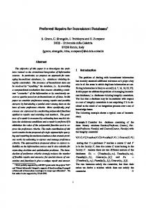
Holistic
Block-wise
Vertex Cover
350
600
300
500
Running Time (sec)
Running Time (sec)
other cells during the partitioning step (i.e., they belong to singleton blocks). Singleton blocks are already clean and do not have to be processed by Algorithm ModGenRepair. This significantly reduces the overhead of inserting clean cells into CleanCells and evaluating whether CleanCells is still clean. Note that limiting the values that can be assigned to t[A] in line 11 to those represented by a new variable comes naturally if Dom(A) is infinite and all values in Dom(A) have equal probability of being the correct replacement of t[A]. The reason is that ignored values (i.e., constants in DomI (A) and variables that have been already used in I 0 ) represent a finite number of values in Dom(A), while a new variable vjA represents an infinite number of values in Dom(A).
250 200 150 400 350 300 250 200 150 50 0 100 100 0
50
20000
40000
0
Greedy
400 300 200 100 0
0
20000
Data Size (tuples)
40000
(a)
0%
10%
20%
30%
Probability of Perturbation
(b)
Figure 7: The Running Time of Generating a Repair.
5.
USER-DEFINED HARD CONSTRAINTS
In this section, we describe a simple modification to Algorithm 2 that generates random repairs with user-defined hard constraints. We consider constraints that specify a set of immutable cells T . Since the algorithm cannot change an immutable cell when generating a repair, we must first ensure that T itself is clean. For this, we build the equivalence relationship E over T using Algorithm 1 and invoke Theorem 1. Here is the modification to Algorithm 2. If T is not clean, we return an empty answer. Otherwise, rather than inserting a random cell into CleanCells at every iteration, we first insert all the cells in T into CleanCells. We know that these cells are clean and that they will not be changed at insertion time. Next, we insert the remaining cells into CleanCells in a random order. We claim that this modification produces repairs in which none of the cells in T are changed since Algorithm 2 always resolves conflicts by only modifying the cell currently being inserted. Figure 5 illustrates an example. Assume that T = {t1 [A], t1 [B], t2 [A], t3 [B]}. In step (a), we insert all the cells in T into CleanCells. The remaining steps show a possible order of insertions and modifications, if needed, of the remaining cells into CleanCells. The end result is a repair that satisfies the hard constraint. On the other hand, if T = {t1 [A], t1 [B], t2 [A], t2 [B]}, then we will find that T is not clean and the algorithm will return an empty answer. Another way of dealing with the case when T is not clean is to relax the hard constraint and allow changes to the cells in T . Here, it is reasonable to return random repairs that minimize the number of changed cells in T . This objective is beyond the scope of this paper and will be pursued in future work.
6.
EXPERIMENTAL STUDY
In this section, we preset an experimental evaluation of our approach. The goal of our experiments is twofold. First, we show that the proposed algorithms can efficiently generate random repairs. Second, we use our repair generator to study the correlation between the number of changes in a repair and the quality of the repair. To provide a reference point, we implemented two previous approaches that deterministically repair FD violations.
6.1
Setup
All experiments were conducted on a SunFire X4100 server with a Dual Core 2.2GHz processor, and 8GB of RAM. All computations are executed in memory. We use synthetic data that is generated by a modified version of the UIS Database generator [1]. This program produces a mailing list that has the following schema: RecordID, SSN, FirstName, MiddleInit, LastName, StNumber, StAddr, Apt,
City, State, ZIP. The following FDs are defined: • SSN → FirstName, MiddleInit, LastName, StNumber, StAddr, Apt, City, State, ZIP • FirstName, MiddleInit, LastName → SSN, StNumber, StAddr, Apt, City, State, ZIP • ZIP → City, State The UIS data generator was originally created to construct mailing lists that have duplicate records. We modified it to generate two instances: a clean instance Ic and another instance Id that is obtained by marking random perturbations to cells in Ic . These perturbations include modifying characters in attributes, swapping the first and last names, and replacing SSNs with all-zeros to indicate missing values. To control the amount of perturbation, we use a parameter Ppert that represents the probability of modifying one or more attributes of each tuple t ∈ Ic . We use four approaches to clean the instance Id that are described as follows. • Holistic: This approach implements Algorithm 2. We tested two versions of the algorithm that execute line 11 in different ways. In the first version, we only allow changing a cell to a new variable (i.e., similar to Algorithm ModGenRepair described in Section 4.2). In the second version, we assume that the three alternatives described in line 11 in Algorithm 2 are equiprobable. • Block-wise: This approach uses Algorithm 3 to partition the input instance into disjoint blocks, followed by Algorithm ModGenRepair to repair individual blocks. • Vertex Cover [12]: This approach is based on modeling FD violations as hyper-edges and using an approximate minimum vertex cover of the resulting hyper-graph to find a repair with a small number of changes. • Greedy RHS [6]: This approach repeatedly picks the violation with the minimum cost to repair and fixes it by changing one or more cells. Modifications are only performed to the right-hand side attributes of the violated FDs.
6.2
Performance Analysis
In Figure 7(a), we show the running time for generating one repair for various data sizes. We only show the running time of the first version of Algorithm Holistic, which is less than or equal to the running time of the second version. We report the average runtime for generating five repairs. For Algorithm Block-wise,
the cost of the initial partitioning of the input instance is amortized over the generated repairs. Algorithm Greedy RHS provides the best scalability, however, at the cost of providing poor output quality. Algorithm Block-wise is ranked second and it outperforms the holistic version of the algorithm by orders of magnitude. For example, repairing 10000 tuples by Algorithm Block-wise took 11 seconds, while Algorithm Holistic took 1450 seconds. Algorithm Vertex Cover is ranked third. We noticed that memory requirements of Algorithm Vertex Cover grow quickly as the number of violations increases due to the large number of the hyper-edges in the initial hyper-graph (e.g., 2.2 million hyper-edges when the input instance contains 15000 tuple). The running times of Algorithms Holistic and Block-wise are almost linear in the number of generated repairs (i.e., the sample size) because the running time for generating a random repair has very low discrepancy. We omit this experiment due to space constraints. Figure 7(b) depicts the running time of the four algorithms for various levels of errors in the input instance, which is captured by the parameter Ppert . Note that Algorithm Holistic incurs a large overhead even when the input database is clean. This is because the algorithm inserts the database cells one-by-one into the set CleanCells and check whether CleanCells is clean upon each insertion. On the other hand, Algorithm Block-wise eliminates such overhead by splitting the input instance into a large number of blocks that can be repaired more efficiently.
6.3
The Relation between the Number of Changes and Quality
In this section, we use our repair sampling algorithm to study the correlation between the number of changes in a repair and the quality of the repair, given that the ground truth is available. Such a study allows for verifying the concept of minimality of changes. For completeness, we also show the characteristics of the repairs generated by other deterministic approaches. We use the precision and recall of the performed changes with respect to the given ground truth as quality metrics. We use the clean instance Ic as the ground truth to assess the quality of a given repair Ir . First, we show how to count the number of correct changes in Ir . We denote by CC(Ir ) the set of cells that are corrected in Ir . CC(Ir ) = {C ∈ ∆(Id , Ir ) : Ir (C) = Ic (C) ∧ Id (C) 6= Ic (C)}
Replacing an incorrect value of a cell in Id (w.r.t. Ic ) with a variable can be considered as a partially correct change. We denote by CV C(Ir ) the set of cells that are partially corrected. CV C(Ir ) = {C ∈ ∆(Id , Ir ) : Ir (C) is a variable ∧ Id (C) 6= Ic (C)}
We define the number of correct changes as the sum of the cardinality of CC(Ir ), and a fraction (0.5 in our experiments) of the cardinality of CV C(Ir ). We assess the quality of Ir using the precision and recall of changes in Ir . We define the precision of a repair Ir as the ratio between the number of correct changes in Ir to the total number of changes in Ir . We define the recall of a repair Ir as the ratio between the number of correct changes in Ir to the number of cells with different values in Ic and Id . In Figure 8, we show the quality of the repairs generated by three algorithms: Block-wise, Vertex Cover, and Greedy RHS. The quality of the repairs generated by Algorithm Holistic is not shown due to space constraints. The input instance consists of 2000 tuples and the parameter Ppert is set to 5%.
Algorithm Block-wise is executed 500 times (due to the randomness of the generating process) , while Algorithms Vertex Cover and Greedy RHS are executed once. The recall of all the algorithms is very low (less than 0.02). The reason is that many errors in Id are not violations of FDs (e.g., errors in the attributes StNumber, StAddr, Apt), and thus they cannot be detected by the cleaning algorithms. Note that we use the entire set of errors in Id to compute the recall (instead of errors that directly contribute to violations of FDs) because there is no unique subset of errors that can be fixed in order to provide a valid repair. Figures 8(a) and 8(b) show the relationship between the number of changes and the precision/recall of the resulting repair. Both precision and recall have strong correlation with the number of changes (-0.95 and -0.68, respectively), which suggests that repairs with fewer changes have superior quality. The first version of Algorithm Holistic provides the same range of precision and recall as Algorithm Block-wise because both algorithms are based on the same repairing semantic (i.e., both are based on Algorithm ModGenRepair). The second version of Algorithm Holistic provides very poor precision and recall (on average 0.05 and 0.006, respectively). The reason is that most of the time, the constants selected at line 11 are different from the correct constant in Ic . This result implies that replacing a cell at line 11 by a variable is safer than picking a random constant that resolves the violation. Note that in Figure 8(c), Algorithm Greedy RHS provides very low precision, compared to the other algorithms. The main reason is that this algorithm performs changes only to the right-hand side attributes of FDs. Thus, errors in left-hand side attributes of FDs are always fixed in the wrong way. For example, missing SSNs are usually replaced by all-zeros. Algorithm Greedy RHS changes all attributes of tuples with missing SSNs to the same value instead of replacing missing SSNs by variables. Algorithm Vertex Cover provides a relatively high precision and recall compared to other approaches (Figure 8(c)). However, a large number of repairs (around 50% of the repairs) generated by Algorithm Block-wise have better quality than those generated by Algorithm Vertex Cover. The reason is that Algorithm Vertex Cover uses an approximate minimum vertex cover to decide which cells are changed (finding an exact minimum vertex cover is NP-hard). We also emphasize that even obtaining a single repair that has the fewest number of changes is not enough because there are several possible repairs that have the same number of changes.
7.
RELATED WORK
In the context of repairing the violations of FDs and other integrity constraints, the most popular approach has been to obtain a single repair via the fewest modifications to the input database (e.g., [6, 12]). Both of these works find a repair whose distance to the input database is close to the optimal distance. The main drawback of single-repair approaches is that there is usually no unique optimal repair. In our work, we address this problem by generating a sample of possible repairs of the input database. Approaches that provide consistent query answers (i.e., answers that are true in every possible repair) perform query rewriting (e.g., [9, 4]), or construct a condensed representation of all repairs that allows obtaining consistent answers [15, 16]. Usually, a restricted class of queries can be answered efficiently while harder classes are answered using approximate methods (e.g., [13]). Our approach overcomes multiple shortcomings of consistent query answering such as returning empty query results when no common query an-
0.02
0.3
0.015
0.1 0
0.015
0.01 0.005
500
Number of Changes
1000
0.025 0.02 0.015 0 015 0.01 0.005 0
0.01 0.005
0 Precision 0.2 0.4
0 0
Greedy RHS
0.02
Recall
0.2
Vertex Cover
Recall call
0.4
Recall call
Precision ision
Block-wise Cleaning
0
500
Number of Changes
((a))
1000
0 0
(b) ( )
0.2
Precision
0.4
(c) ( )
Figure 8: The Quality of the Generated Repairs. swers are found. In [10], the authors proposed a model of possible repairs of inconsistent databases. The proposed model imposes a strong constraint on the defined FDs. Specifically, any attribute that appears in the right-hand side of an FD cannot appear in the left-hand side of another FD. In this setting, FD violations can be repaired independently and cardinality-minimal repairs can be obtained in PTIME. Our solutions apply to arbitrary sets of FDs. A related problem is checking whether a given instance is a repair of the input instance. For example, in [3], authors studied the complexity of deciding whether a specific instance is a minimal repair (under several semantics of minimality) for larger classes of integrity constraints. New definitions of minimality are also proposed in [3] such as component cardinality repairs, which generalize cardinality-minimal repairs of database instances that consist of multiple relations (i.e., components) in the sense that repairs that are Pareto-optimal w.r.t. the number of changes in each component are considered as possible repairs, even if the total number of changes is not minimal. Such generalization is not useful in the class of FDs because individual relations are repaired independently and thus component cardinality repairs are equivalent to cardinality-minimal repairs. A related topic to or work is answering queries over uncertain data. Many works have addressed the problem of modeling data uncertainty in a compact way to allow efficient query answering (e.g., [5, 14]). One of the related works is the Monte-Carlo Database (MCDB) [11], which allows answering user queries efficiently using a sample of possible realizations (i.e., possible worlds) of a database by avoiding redundant computations. For example, query planning is performed only once for the entire set of possible repairs. We envision integrating our repair-generating algorithms with MCDB to facilitate efficient query answering.
8.
CONCLUSION
In this paper, we presented a new technique for constraint-based database repair, in which we generate a random sample of the possible repairs. We described a realization of this technique in the context of Functional Dependencies, given a novel repair space that combines the features of two well-known existing spaces: set and cardinality minimal. We also extended our sampling algorithm to allow user-defined hard constraints that specify a set of cells that must remain unchanged during the repairing process. Our experimental study indicates that partitioning the input instance into blocks that can be repaired independently results in orders of magnitude performance gain. An important direction for future work is to design new repair sampling algorithms for other types of integrity constraints and data quality rules, and understand the corresponding repair spaces.
9.
REFERENCES
[1] UIS data generator, http://www.cs.utexas.edu/users/ml/riddle/data.html. [2] S. Abiteboul, R. Hull, and V. Vianu. Foundations of Databases. Addison-Wesley, 1995. [3] F. N. Afrati and P. G. Kolaitis. Repair checking in inconsistent databases: algorithms and complexity. In ICDT, pages 31–41, 2009. [4] M. Arenas, L. E. Bertossi, and J. Chomicki. Consistent query answers in inconsistent databases. In PODS, pages 68–79, 1999. [5] O. Benjelloun, A. D. Sarma, A. Y. Halevy, and J. Widom. ULDBs: Databases with uncertainty and lineage. In VLDB, pages 953–964, 2006. [6] P. Bohannon, M. Flaster, W. Fan, and R. Rastogi. A cost-based model and effective heuristic for repairing constraints by value modification. In SIGMOD, pages 143–154, 2005. [7] J. Chomicki and J. Marcinkowski. Minimal-change integrity maintenance using tuple deletions. Information and Computation, 197(1/2):90–121, 2005. [8] J. Chomicki, J. Marcinkowski, and S. Staworko. Computing consistent query answers using conflict hypergraphs. In CIKM, pages 417–426, 2004. [9] A. Fuxman and R. J. Miller. First-order query rewriting for inconsistent databases. Journal of Computer and System Sciences, 73(4):610–635, 2007. [10] S. Greco and C. Molinaro. Approximate probabilistic query answering over inconsistent databases. In ER, pages 311–325, 2008. [11] R. Jampani, F. Xu, M. Wu, L. L. Perez, C. M. Jermaine, and P. J. Haas. MCDB: a monte carlo approach to managing uncertain data. In SIGMOD, pages 687–700, 2008. [12] S. Kolahi and L. V. S. Lakshmanan. On approximating optimum repairs for functional dependency violations. In ICDT, pages 53–62, 2009. [13] A. Lopatenko and L. E. Bertossi. Complexity of consistent query answering in databases under cardinality-based and incremental repair semantics. In ICDT, pages 179–193, 2007. [14] P. Sen and A. Deshpande. Representing and querying correlated tuples in probabilistic databases. In ICDE, pages 596–605, 2007. [15] J. Wijsen. Condensed representation of database repairs for consistent query answering. In ICDT, pages 375–390, 2003. [16] J. Wijsen. Database repairing using updates. ACM Trans. Database Syst., 30(3):722–768, 2005.
I
APPENDIX A.
RANDOMIZATION OF PREVIOUS APPROACHES
In this section, we give counterexamples to illustrate why previous approaches that produce a single repair (e.g., [6, 12]) are not suitable for generating a random sample of repairs.
I A
B
C
D
E
t1
1
1
2
3
6
7
t2
1
1
1
4
7
8
t3
2
2
1
5
8
A
B
C
D
E
t1
1
1
2
3
6
t2
1
1
1
4
t3
2
2
1
5
Initial a doub double e co conflicts cs
Σ= {AÆB, BÆC, CÆD, DÆE}
Initial a triple p e co conflicts cs
(a)
I’
I t1 t2 t3
A 1 1 2
B 4 1 1
C 2 2 3
t1 t2 t3
A 1 1 2
B 4 1 1
C 2 2 2
t1 t2 t3
A 1 1 2
B 4 4 1
I’
C 2 2 2
Σ= {AÆB , BÆC} Σ
C
D
E
t1
1
1
2
3
6
t2
1
1
2
3
6
t3
2
2
1
5
8
(b) Figure 10: An Example of a Cardinality-minimal Repair that Cannot Be Generated by the Algorithm in [12].
B.
COMPLEXITY ANALYSIS OF ALGORITHM 2
Let n be the number of tuples in the input instance I, and m be the number of attributes in I. In Algorithm 1, the maximum number of merges of equivalence classes is less than or equal to the number of distinct tuples that appear in C multiplied by the number of distinct attributes in C. Therefore, the complexity of Algorithm 1 is in O(n · m). Evaluating IsClean can be done in O(m · n log n) by sorting the cells of each attribute based on their equivalence classes and ensuring that cells in each equivalence class have the same value. In Algorithm 2, the number of iterations is equal to the number of cells in I 0 (i.e., n · m). In each iteration, Algorithm 1 is invoked to build the equivalence classes of cells in CleanCells. Additionally, in line 11, Algorithm 1 and the condition IsClean can be evaluated for all possible constants and variables that appear in the attribute A in I 0 (in worst case). Hence, the complexity of each iteration is O(m · n2 log n) and the overall complexity of Algorithm 2 is O(m2 · n3 log n).
C. We show that some cardinality-minimal repairs cannot be generated by the approach presented in [12]. We illustrate such a fact using the example in Figure 10. In Figure 10(a), we show the hyperedges (also called double and triple conflicts) that exist in the initial conflict graph. We note that the algorithm in [12] can only change a cell t[Ai ] if it appears in the initial conflict graph, or there exists an FD X → Aj ∈ Σ such that Ai ∈ X and t[Aj ] appears in the initial conflict graph. It follows that the cell t2 [E] in Figure 10 can never be changed by the algorithm. Therefore, the cardinality-minimal repair I 0 that is shown in Figure 10(b) cannot be generated by the algorithm in [12]. Some cardinality-minimal repairs cannot be generated by the algorithm in [12] because the algorithm is biased towards replacing the cells that belong to the left-hand side attributes of FDs with new variables (step 2 of the algorithm presented in [12]). In our algorithm, we consider all possible values when changing a given cell that is involved in a violation as we describe in Section 4.
B
A Cardinality-minimal Repair
Figure 9: An Example of a Repair Generated by the Algorithm in [6] that is Not Set-minimal. First, we show that the algorithm introduced in [6] may generate repairs that are not set-minimal (i.e., contain unnecessary changes). The algorithm repairs an input instance by repeatedly searching for tuples that violate a certain FD X → A ∈ Σ and modify the attribute A of the violating tuples to have the same value. For example, in Figure 9, we show a possible repair I 0 of the input instance I that can be generated by the algorithm in [6]. Modified cells are shaded in the figure. The fist step repairs a violation of B → C by associating the cells t2 [C] and t3 [C] to the same equivalence class and changing the cell t3 [C] to 2. In the second step, a violation of A → B is fixed by changing t2 [B] to 4. The resulting repair I 0 is not set-minimal because the cell t3 [C] can be reverted to its value in I without violating any FD. Repairs that are not set-minimal can be generated by the algorithm in [6] due to the fact that the generated repairs can involve contradicting assumptions. For example, the cell t2 [B] is used in the first step for changing t3 [C] to 2 (i.e., t2 [B] is assumed to be a correct cell). In the second step, t2 [B] is modified to 4, which implies that t2 [B] is incorrect (i.e., unclean). We avoid such contradictions in our algorithm that is presented in Section 4. That is, once a cell Ci is used for modifying another cell Cj , Ci cannot be modified any further. We enforce this constraint by avoiding changing cells that are already in the set CleanCells and only changing the cell currently being inserted (refer to Algorithm 2).
A
PROOFS
C.1
Proof of Lemma 1
For any two repairs I 0 and I 00 of I, ∆(I, I 00 ) ⊂ ∆(I, I 0 ) → |∆(I, I 00 )| < |∆(I, I 0 )| This implies that for any repair I 0 of I, @I 00 ∈ Repairs(I) (|∆(I, I 00 )| < |∆(I, I 0 )|) → @I 00 ∈ Repairs(I) (∆(I, I 00 ) ⊂ ∆(I, I 0 )) Therefore, if I 0 is a cardinality-minimal repair, I 0 is cardinalityset-minimal. Similarly, for any two repairs I 0 and I 00 of I, ∆(I, I 00 ) ⊂ ∆(I, I 0 ) ∧ ∀C ∈ ∆(I, I 00 ) (I 00 (C) = I 0 (C)) → ∆(I, I 00 ) ⊂ ∆(I, I 0 )
Therefore, if I 0 is a cardinality-set-minimal repair, I 0 is setminimal.
C.2
Proof of Theorem 1
We prove the “only if” direction as follows. Let I be a subset of repairs of I such that ∀I 0 ∈ I (∀C ∈ C, I 0 (C) = I(C)). We first prove that whenever two cells belong to the same equivalence class, they must have equal values in every I 0 ∈ I. We provide a recursive proof as follows. If two cells t[A] and t0 [A] belong to the same equivalence class, then either I(t[A]) = I(t0 [A]) and thus I 0 (t[A]) = I 0 (t0 [A]), or there exists an FD X → A ∈ Σ such that for all B ∈ X, t[B] and t0 [B] belong to the same equivalence class. Recursively, we can prove that for all B ∈ X, I 0 (t[B]) = I 0 (t0 [B]). Furthermore, I 0 |= X → A implies that I 0 (t[A]) = I 0 (t0 [A]). If there exist two cells Ci and Cj in C that belong to the same equivalence class while having different values in I, no repair I 0 can satisfy I 0 (Ci ) = I 0 (Cj ) and I 0 (Ci ) 6= I 0 (Cj ) simultaneously. Thus, the set I is empty in this case (i.e., cells in C are unclean). We prove the “if” direction as follows. Consider the case where @Ci , Cj ∈ C (ec(E, Ci ) = ec(E, Cj ) ∧ I(Ci ) 6= I(Cj )). We need to prove that the set I is not empty. Let I 0 be an instance where ∀C ∈ C, I 0 (C) = I(C) and the values of cells in CIDs(I 0 )\C are set as follows. Each cell in a non-singleton equivalence class is set to the value of the other cells in the equivalence class. Each cell that belong to a singleton equivalence class, or is not associated with an equivalence class is set to a distinct variable. In other words, I 0 is constructed such that cells that have equal values in I 0 must belong to the same equivalence class, and vice versa. For every two tuples t, t0 ∈ I 0 and for every FD X → A ∈ Σ, t[X] = t0 [X] implies that for all B ∈ X, t[B] and t0 [B] belong to the same equivalence class. Therefore, t[A] and t0 [A] must belong to the same equivalence class as well (based on Algorithm 1, lines 8-10), and thus I 0 (t[A]) = I 0 (t0 [A]). This proves that I 0 |= Σ and thus I is not empty (i.e., cells in C are clean).
C.3
Proof of Theorem 2
We need to prove the following points: 1. Every generated instance I 0 is a repair of I w.r.t Σ. 2. Every generated repair I 0 is set-minimal. 3. All cardinality-set-minimal repairs can be generated by the algorithm. To prove the first point, we show that all the cells of the generated instance I 0 are clean. We prove this point by induction. In the base case, CleanCells contains one cell, and thus the set of cells CleanCells in the instance I 0 are clean. We need to prove in the induction step that if the cells CleanCells in I 0 are clean, CleanCells ∪ {t[A]} in I 0 are clean as well, for any cell t[A] 6∈ CleanCells that is possibly changed to another value according to the lines 6-13 in Algorithm 2. That is, either the set CleanCells ∪ {t[A]} is clean for I 0 (t[A]) = I(t[A]), or I 0 (t[A]) is changed in a way that makes the set CleanCells ∪ {t[A]} clean. We concentrate on the latter case. Let Ep be the set of equivalence classes that is constructed based on the set CleanCells, and E be the set of equivalence classes that is constructed based on the set CleanCells ∪ {t[A]} after changing t[A] based on lines 6-13 in the algorithm. There are two possible scenarios, which we describe as follows. • t[A] belongs to a non-singleton equivalence class E ∈ E such that E contains other cells previously inserted in CleanCells. In this case, setting t[A] in I 0 to the values
of other cells in E does not violate the constraints imposed by Ep . Also, such change implies that E = Ep . It follows that CleanCells ∪ {t[A]} is clean. • t[A] belongs to a non-singleton equivalence class that only contains t[A], or t[A] belongs to a singleton class. In this case, we set t[A] to a constant or a variable that appears in I 0 such that CleanCells ∪{t[A]} is clean. Alternatively, we set t[A] to a new variable vjA . In the latter case, the constraints imposed by Ep are not violated because vjA cannot be in the same equivalence class of any other cell in CleanCells. Moreover, setting vjA does not result in merging the equivalence class ec(Ep , t[A]) with any other classes (i.e., E = Ep ). Thus, CleanCells ∪ {t[A]} is clean. Upon termination of the algorithm, the set CleanCells contains all cells of I 0 . Therefore, I 0 is a repair of I. To prove the second point, we need to show that any subset of the changed cells ∆(I, I 0 ) cannot be reverted to their values in I without violating Σ. We say that a cell C in ∆(I, I 0 ) represents a necessary change in a repair I 0 if we cannot revert any subset of ∆(I, I 0 ) that contains C without violating Σ. A repair I 0 is setminimal if every cell in ∆(I, I 0 ) represents a necessary change. Let C1 , C2 , . . . , Cβ be the order in which cells are inserted into CleanCells in Algorithm 2, where β = |CIDs(I)|. We prove by strong induction that every cell Ci , 1 ≤ i ≤ β is either an unchanged cell or a changed cell that represents a necessary change. • The base case: The set {C1 } is a clean set of cells, and thus C1 remains unchanged. • The induction step: We show that if every cell in {C1 , . . . , Ci } is either an unchanged cell or a necessarily changed cell, Ci+1 is either unchanged or a necessarily changed cell. If Ci+1 is unchanged, the induction step is correct. Otherwise, Ci+1 is changed and we need to show that changing Ci+1 is necessary. We prove this fact by contradiction. Assume that ∃S ⊆ ∆(I, I 0 ) such that Ci+1 ∈ S and we can revert cells in S to the their original values in I without violating Σ. All changed cells in {C1 , . . . , Ci } represent necessary changes, and thus S ∩ {C1 , . . . , Ci } = φ. It follows that for I 0 (Ci+1 ) = I(Ci+1 ) (i.e., Ci+1 is unchanged), the set {C1 , . . . , Ci+1 } in I 0 is not conflicting. However, in this case, Algorithm 2 would not change Ci+1 , a contradiction. It follows that every cell in ∆(I, I 0 ) represents a necessary change, which implies that I 0 is set-minimal. In the third point, we show that Algorithm 2 can generate all cardinality-set-minimal repairs. Algorithm 2 involves two types of randomness: the order in which cells are inserted into the set CleanCells (line 4), and the values that are assigned to unclean cells in line 11. In the following, we show that for every cardinalityset-minimal repair I 0 , there exist an order of cells and a set of new values of unclean cells that are considered by Algorithm 2 in order to generate I 0 . Let C1 , . . . , Cα be any arbitrary order of the unchanged cells in I 0 , where α = |CIDs(I)| − |∆(I, I 0 )|. Let Cα+1 , . . . , Cβ be an arbitrary order of the changed cells in I 0 , where β = |CIDs(I)|. Let I be the set of repairs that can be generated by Algorithm 2 when inserting the cells into CleanCells in the order C1 , . . . , Cα , Cα+1 , . . . , Cβ . We show that I 0 ∈ I by contradiction. Assume that I 0 6∈ I. For each I 00 ∈ I, let δ(I 00 ) be the index of the first cell that has different values in I 0 and I 00 . That is, δ(I 00 ) = min({i : I 0 (Ci ) 6=
I 00 (Ci )}). For all I 00 ∈ I, δ(I 00 ) > α because C1 , . . . , Cα are clean (i.e., there exist at least one repair of I, which is I 0 , such that C1 , . . . , Cα are unchanged). Thus, Algorithm 2 will not change any cell in C1 , . . . , Cα . Also, for all I 00 ∈ I, δ(I 00 ) ≤ β because no repair I 00 ∈ I can be identical to I 0 (based on our assumption). Let Im be the repair in I with the maximum δ(.), i.e., Im = maxarg I 00 ∈I δ(I 00 ). Because I 0 is cardinality-set-minimal and the cells {C1 , . . . , Cα } are unchanged in I 0 as well as all repairs in I, the cells {Cα+1 , . . . , Cβ } must be changed in every repair in I. Therefore, the cell Cδ(Im ) must have been changed in Im by the algorithm, i.e., Im (Cδ(Im ) ) 6= I(Cδ(Im ) ). This implies that C1 , . . . , Cδ(Im ) in Im are not clean when Cδ(Im ) is unchanged (i.e., Im (Cδ(Im ) ) = I(Cδ(Im ) )). The value I 0 (Cδ(Im ) ) is a possible assignment to Cδ(Im ) that is considered by Algorithm 2 at either line 9 or line 11 in order to make C1 , . . . , Cδ(Im ) clean. Therefore, there must exist Ip ∈ I such that Ip (Ci ) = Im (Ci ) for 1 ≤ i < δ(Im ) and Ip (Cδ(Im ) ) = I 0 (Cδ(Im ) ). This implies that δ(Ip ) > δ(Im ), which contradicts the fact that Im = maxarg I 00 ∈I δ(I 00 ). It follows that our initial assumption is incorrect (i.e., every cardinality-set-minimal repair I 0 can be generated by Algorithm 2).
C.4
Proof of Theorem 3
We first prove that for any repair I 0 generated by Algorithm ModGenRepair(I, Σ), every equivalence class in E 0 = BuildEquivRel(CIDs(I 0 ), I 0 , Σ) is contained in another equivalence class in E = BuildEquivRel(CIDs(I), I, Σ). We approach our proof by induction. We denote by CleanCellsi the value of the set CleanCells at iteration i of the algorithm, and denote by Ei the equivalence relation returned by the procedure BuildEquivRel(CleanCellsi , I 0 , Σ). Initially, the set CleanCells1 contains one unchanged cell. Therefore, E1 contains one singleton equivalence class that is contained in an equivalence class in E. At iteration i in the algorithm, assume that for each E 0 ∈ Ei−1 , ∃E ∈ E such that E 0 ⊆ E. An additional cell C is added to CleanCellsi−1 , resulting in the set CleanCellsi . If C is unchanged during the current iteration, C will be either associated to the same equivalence class in Ei−1 , or be associated to another class E 00 ∈ Ei−1 . In the former case, Ei = Ei−1 and thus the relationship between Ei and E is similar to the relationship between Ei−1 and E. In the latter case, the class E 00 is contained in some class E in E. Additionally, the first cell that is inserted into CleanCells and belongs to E 00 is unchanged and its value is equal to I(C). Thus, the cell C must belong to E after executing BuildEquivRel(CIDs(I), I, Σ), which implies that E 00 ∪ {C} ⊆ E. Now, we consider the case where C is changed. Algorithm ModGenRepair can only change C such that Ei = Ei−1 . At the final iteration, Ei = E 0 , which proves that ∀E 0 ∈ E 0 (∃E ∈ E, E 0 ⊆ E). A direct result is that the possible constant values of a cell t[A] in any randomly generated repair I 0 of I, denoted P VI (t[A]), are values of the cells in the equivalence class ec(E, t[A]) in the input instance I. Therefore, for two cells t[A] and t0 [A] that belong to different equivalence classes in E, P VI (t[A]) ∩ P VI (t0 [A]) = φ. Based on Algorithm 3, for every FD X → A and for every two tuples t, t0 such that t[X] and t0 [X] belong to different blocks, P VI (t[X]) ∩ P VI (t0 [X]) = φ. Assume that I is partitioned into multiple blocks P1 , P2 , . . . using Algorithm 3 and that Pi0 is a repair of Pi . Denote by P VP (t[X]) the possible values of attributes X of a tuple t in a randomly generated repair P 0 of a block P . P VP (t[X]) ⊆ P VI (t[X]) because repairing P can be considered as an initial
step of repairing I, where all cells in P are inserted first into CleanCells. Therefore, for every FD X → A and for every two sets t[X] ∈ Pi and t0 [X] ∈ Pj for i 6= j, P VPi (t[X]) ∩ P VPj (t0 [X]) = φ. Hence, P10 ∪ P20 ∪ . . . satisfies all FDs in Σ (i.e., the instance resulting from merging P10 , P20 , . . . represents a repair of I).