In this research paper, we discuss Sapa, a domain-independent heuristic ..... which the fact/action can be achieved/executed, and the lowest cost incurred to ...
Sapa: A Scalable Multi-objective Heuristic Metric Temporal Planner Minh B. Do, Subbarao Kambhampati ∗ Department of Computer Science and Engineering Arizona State University, Tempe AZ 85287-5406 {binhminh,rao}@asu.edu
Abstract In this research paper, we discuss Sapa, a domain-independent heuristic forward chaining planner that can handle durative actions, metric resource constraints, and deadline goals. It is designed to be capable of handling the multi-objective nature of the metric temporal planning. Our technical contributions include discussion of (i) various objective functions for planning and the multi-objective search framework (ii) a planning-graph based method for deriving heuristics that are sensitive to both cost and makespan (iii) an easy way of adjusting the heuristic estimates to take the metric resource limitations into account and (iv) a linear time greedy post-processing technique to improve the solution’s execution flexibility and quality according to given criteria. An implementation of Sapa using a subset of the techniques presented in this paper was one of the best domain independent planners for domains with metric and temporal constraints in the third International Planning Competition, held at AIPS-02. We describe the technical details of extracting the heuristics and present an empirical evaluation of the current implementation of Sapa.
1 Introduction The success of the Deep Space Remote Agent experiment has demonstrated the promise and importance of scalable metric temporal planning for NASA applications. HSTS/RAX, the planner used in the remote agent experiment, was predicated on the availability of domain- and planner-dependent control knowledge, the collection and maintenance of which is admittedly a laborious and error-prone activity. An obvious question of course is whether it will be possible to develop domain-independent metric temporal planners that are capable of scaling up to such domains. The past experience has not particularly been encouraging. Although there have been some ambitious attempts–including IxTeT [18] and Zeno [32], their performance has not been particularly satisfactory. Some encouraging signs however are the recent successes of domain-independent heuristic planning techniques in classical planning (c.f. AltAlt [29] HSP [4] and FF [20]). Our research is ∗
We thank Daniel Bryce for developing the GUI for Sapa. This research is supported in part by the NSF grant IRI-9801676, and the NASA grants NAG2-1461 and NCC-1225.
1
aimed at building on these successes to develop a scalable metric temporal planner. At first blush search control for metric temporal planners would seem to be a very simple matter of adapting the work in heuristic planners in classical planning [4, 29, 20]. The adaptation however does pose several challenges: • Metric temporal planners tend to have significantly larger search spaces than classical planners. After all, the problem of planning in the presence of durative actions and metric resources subsumes both the classical planning and scheduling problems. • Compared to classical planners, which only have to handle the logical constraints between actions, metric temporal planners have to deal with many additional types of constraints that involve time and continuous functions representing different aspects of resource. • In contrast to classical planning, where the only objective is to find shortest length plans, metric temporal planning is multi-objective. The user may be interested in improving either temporal quality of the plan (e.g. makespan) or its cost (e.g. cumulative action cost, cost of resources consumed etc.), or more generally, a combination there of. Consequently, effective plan synthesis requires heuristics that are able to track both these aspects in an evolving plan. Things are further complicated by the fact that these aspects are often interdependent. For example, it is often possible to find a “cheaper” plan for achieving goals, if we are allowed more time to achieve them. In this paper, we present Sapa, a heuristic metric temporal planner that we are currently developing, to overcome these challenges. Sapa is a forward chaining metric temporal planner, which searches in the space of time-stamped states (see below [1]). Sapa handles durative actions as well as actions consuming continuous resources. Our main focus has been on the development of heuristics for focusing Sapa’s multi-objective search. These heuristics are derived from the optimistic reachability information encoded in the planning graphs. Unlike classical planning heuristics (c.f. AltAlt [29]), which need only estimate the “length” of the plan needed to achieve a set of goals, Sapa’s heuristics need to be sensitive to both the cost and length (“makespan”) of the plans for achieving the goals. Our contributions include: • We present a novel framework for tracking the cost of literals (goals) as a function of time. These “cost functions” are then used to derive heuristics that are capable of driving the search towards plans that satisfy any type of cost-makespan tradeoffs. • Sapa generalizes the notion of “phased” relaxation used in deriving heuristics in planners such as AltAlt and FF [29, 20]. Specifically, the heuristics are first derived from a relaxation that ignores the delete effects and metric resource constraints, and are then adjusted subsequently to better account for both negative interactions and resource constraints. • While Sapa’s forward-chaining search in the time-stamped states results in position-constrained plans, it improves the temporal flexibility of the solution plans by post-processing the position-constrained plans to produce equivalent “precedence-constrained” plans. This way, Sapa is able to exploit both the ease of resource reasoning offered by the positionconstrained plans and the execution flexibility offered by the precedence-constrained plans. 2
We discuss and implement the linear time greedy approach to generate an o.c plan of better or equal makespan value compare to the original p.c plan. This approach can be thought of as a specific variable and value ordering for the CSOP encoding discussed in [10]. A version of Sapa using a subset of the techniques discussed in this paper was one of the best domain independent planners for domains with metric and temporal constraints in the third International Planning Competition, held at AIPS 2002[13]. In fact, it is the best planner in terms of solution quality and number of problems solved in the highest level of PDDL2.1 used in the competition for the domains Satellite and Rovers. These domains are both inspired by NASA applications. The paper is organized as follows: in Section 2 we discuss the forward state space search algorithm to produce concurrent metric temporal plans with durative actions. In that section, Section 2.1 is used to describe the action representation and constraints; and Section 2.2 concentrates on the forward chaining algorithm. Next, in Section 3, we discuss the problem of how to build a temporal planning graph and use it to propagate the time and cost information (time-sensitive cost functions). Section 4 shows how the propagated information can be used to estimate the cost of achieving the goals from a given state. We also discuss in that section how the ignored mutual exclusion relations and resource information help improve the heuristic estimation. To improve the quality of the solution, Section 5 discusses our greedy approach of building the order constrained plan (aka. partial order plan) from parallel position constrained plans returned by Sapa. Section 6 discusses the implementation of Sapa, presents some empirical results of Sapa in producing plans with tradeoff for cost and makespan, and analyzes its performance in the international planning competition. We conclude the paper with a discussion on related work in Section 7 and on the conclusion in Section 8.
2 Handling concurrent actions in a forward state space planner Sapa addresses planning problems that involve durative actions, metric resources, and deadline goals. In this section, we describe how such planning problems are represented and solved in Sapa. We first describe the action representation, and will then present the forward chaining state search algorithm used by Sapa.
2.1 Action Representation & Constraints Planning is the problem of finding a set of actions and their respective execution times to satisfy all causal, metric, and resource constraints. Therefore, action representation has influences on the representation of the plans and on the planning algorithm. In this section, we will briefly describe the PDDL2.1 Level 3 action representation, which is the highest level (in terms of the expressiveness of temporal and metric resource constraints) used in the third international competition. Sapa is able to solve problems in PDDL2.1 Level 3 and was one of the best of such planners in the competition.1 1 The original action representation used in Sapa is slightly different from the PDDL2.1 Level 3. However, we will commit to the standard action representation from now on.
3
Train Las Vegas LA
Tucson Car1 Car2
Phoenix Airplane
Figure 1: The travel example Unlike actions in classical planning, in planning problems with temporal and resource constraints, actions are not instantaneous but have durations. Each action A has a duration DA , starting time SA , and end time (EA = SA + DA ). The value of DA can be statically defined for a domain, statically defined for a particular planning problem, or can be dynamically decided at the time of execution.2 An action A can have preconditions P re(A) that may be required either to be instantaneously true at the time point SA , or required to be true starting at SA and remain true for some duration d ≤ DA . The logical effects Eff(A) of A will be divided into two sets Es (A), and Ee (A) containing, respectively, the instantaneous effects at time points SA , and EA . Actions can also consume or produce metric resources and their preconditions may also depend on the value of the corresponding resource. For resource related preconditions, we allow several types of equality or inequality checking including ==, , =. For resourcerelated effects, we allow the following types of change (update): assignment(=), increment(+=), decrement(-=), multiplication(*=), and division(/=). We shall now illustrate the action representation in a simple temporal planning problem. This problem will be used as the running example through out the rest of the paper. Figure 1 shows graphically the problem description. In this problem, a group of students in Tucson need to go to Los Angeles (LA). Between two options of renting a car, if the students rent a faster but more expensive car (Car1), they can only go to Phoenix (PHX) or Las Vegas (LV). However, if they decide to rent a slower but cheaper Car2, then they can use it to drive to Phoenix or directly to LA. Moreover, to reach LA, the students can also take a train from LV or a flight from PHX. In total, there are 6 movement actions in the domain: drive-car1-tucson-phoenix c1 c1 , Dur = 1.0, Cost = 2.0), drive-car1-tucson-lv (Dt→lv , Dur = 3.5, Cost = 3.0), drive(Dt→p c2 c2 ),Dur = 7.0, car2-tucson-phoenix (Dt→p , Dur = 1.5, Cost = 1.5), drive-car2-tucson-la (Dt→la Cost = 6.0, fly-airplane-phoenix-la (Fp→la , Dur = 1.5, Cost = 6.0), and use-train-lv-la (Tlv→la , Dur = 2.5, Cost = 2.5). Each move (by car/airplane/train) action A between two cities X and Y requires the precondition that the students be at X (at(X))at the beginning of A. There are 2
For example, in the traveling domain discussed in this section, we can decide that boarding a passenger always takes 10 minutes for all problems in this domain. Duration of the action of flying an airplane between two cities will depend on the distance between these two cities and the speed of the airplane. Because the distance between two cities will not change over time, the duration of a particular flying action will be totally specified once we parse the planning problem. However, refueling an airplane may have a duration that depends on the current fuel level of that airplane. We may only be able to calculate the duration of a given refueling action according to the fuel level at the exact time instant when we execute that action.
4
also two temporal effects: ¬at(X) occurs at the starting time point of A and at(Y ) at the end time point of A. Driving and flying actions also consume different types of resource (e.g fuel) at different rates depending on the specific car or airplane used. In addition, there are refueling actions for cars and airplanes. The durations of the refueling actions depend on the amount of fuel remaining in the vehicle and the refueling rate. The summaries of action specifications for this example are shown on the right side of Figure 1. In this example, the costs of moving by train or airplane are the respective ticket prices, and the costs of moving by rental cars include the rental fees and gas (resource) costs.
2.2 A Forward Chaining Search Algorithm for metric temporal planning Even though variations of the action representation scheme described in the previous section have been used in the partial order temporal planners such as IxTeT[18] and Zeno[32] before, Bacchus and Ady [1] are the first to propose a forward chaining algorithm capable of using this type of action representation allowing concurrent execution of actions in the plan. We adapt their search algorithm in Sapa. Sapa’s search is conducted through the space of time stamped states. We define a time stamped state S as a tuple S = (P, M, Π, Q, t) consisting of the following structure: • P = (�pi , ti � | ti < t) is a set of predicates pi that are true at t and the last time instant ti at which they are achieved. • M is a set of values for all continuous functions, which may change over the course of planning. Functions are used to represent the metric-resources and other continuous values. Examples of functions are the fuel levels of vehicles. • Π is a set of persistent conditions, such as durative preconditions, that need to be protected during a specific period of time. • Q is an event queue containing a set of updates each scheduled to occur at a specified time in the future. An event e can do one of three things: (1) change the True/False value of some predicate, (2) update the value of some function representing a metric-resource, or (3) end the persistence of some condition. • t is the time stamp of S In this paper, unless noted otherwise, when we say “state” we mean a time stamped state. It should be obvious that time stamped states do not just describe world states (or snap shots of the world at a given point of time) as done in classical progression planners, but rather describe both the current state of the world and the state of the planner’s search (set of events/changes that are guaranteed to occur given the actions in the current plan). The initial state Sinit is stamped at time 0 and has an empty event queue and empty set of persistent conditions. It is completely specified in terms of function and predicate values. The goals are represented by a set of 2-tuples G = (�p1 , t1 �...�pn , tn �) where pi is the ith goal and ti is the time instant by which pi needs to be achieved. Note that PDDL2.1 still does not
5
allow the specification of goal deadline constraints. Therefore, we currently use our original representation for problems requiring goal deadline constraints. We intend to extend PDDL2.1 in the near future to include goal deadlines and other types of temporal constraints. Goal Satisfaction: The state S = (P, M, Π, Q, t) subsumes (entails) the goal G if for each �pi , ti � ∈ G either: 1. ∃�pi , tj � ∈ P , tj < ti and there is no event in Q that deletes pi . 2. ∃e ∈ Q that adds pi at time instant te < ti . Action Application: An action A is applicable in state S = (P, M, Π, Q, t) if: 1. All logical (pre)conditions of A are satisfied by P. 2. All metric resource conditions of A are satisfied by M.3 3. A’s effects do not interfere with any persistent condition in Π and any event in Q. 4. � ∃e ∈ Q interferes with persistent preconditions of A. The interference relation between action A’s effects, event queue Q, and the persistent condition Π follow the interference rules defined in PDDL2.1. In short, they are: • If A deletes a proposition p and there is an event e in Q that adds p, then A can not delete P at the same time instant at which that event occurs (epsilon or higher duration should separate two events). • If A deletes p and p is protected in Π until time point tp , then A should not delete p before tp . • If A has a persistent precondition p, and there is an event that gives ¬p, then that event should occur after A terminates. • A should not change the value of any function (representing a resource) which is used to satisfy a (pre)condition of another unterminated action4 . Moreover, if A has a precondition that depends on the value of some function that is changed as an effect of an unterminated action A� , then A also interferes with that action (and is not applicable at the current state). When we apply an action A to a state S = (P, M, Π, Q, t), all instantaneous effects of A will be immediately used to update the predicate list P and metric resources database M of S. A’s persistent preconditions and delayed effects will be put into the persistent condition set Π and event queue Q of S. For example, if the condition to execute an action A = move(truck, A, B) is f uel(truck) > 500 then A is executable in S if the value v of f uel(truck) in M satisfy v > 500. 4 Unterminated actions are the ones that started before the time point t of the current state S but have not yet finished at t. 3
6
State Queue: SQ={Sinit } while SQ�={} S:= Dequeue(SQ) Nondeterministically select A applicable in S S’ := Apply(A,S) if S’ satisfies G then PrintSolution else Enqueue(S’,SQ) end while; Figure 2: Main search algorithm Besides the normal actions, we will have a special action called advance-time5 which we use to advance the time stamp of S to the time instant te of the earliest event e in the event queue Q of S. The advance-time action will be applicable in any state S that has a non-empty event queue. Upon applying this action, the state S gets updated according to all the events in the event queue that are scheduled to occur at te . Search algorithm: The basic algorithm for searching in the space of time stamped states is shown in Figure 2. We proceed by applying all applicable actions to the current state and put the result states into the sorted queue using the Enqueue() function. The Dequeue() function is used to take out the first state from the state queue. Currently, Sapa employs the A* search. Thus, the state queue is sorted according to some heuristic function that measures the difficulty of reaching the goals from the current state. The rest of the paper discusses the design of such heuristic functions.
3 Propagating time-sensitive cost functions using the temporal planning graphs In this section, we discuss the issue of deriving heuristics, that are sensitive to both time and cost, to guide Sapa’s search algorithm. An important challenge in finding heuristics to support multi-objective search, as illustrated by the example below, is that the cost and temporal aspects of a plan are often inter-dependent. Therefore, in this section, we introduce the approach to track the cost of achieving goals and execute actions in the plan as the functions of time. Then, the propagated cost functions can be used to derive the heuristic values to guide the search in Sapa. Example: Let’s take a simpler version of our ongoing example. Suppose that we need to go from Tucson to Los Angeles. The two common options are: (i) rent a car and drive from Tucson to Los Angeles in one day for $100 or (ii) take a shuttle to the Phoenix airport and fly to Los Angeles in 3 hours for $200. The first option takes more time (higher makespan) but less money, while the second one clearly takes less time but is more expensive. Depending on the specific weights the user gives to each criterion, she may prefer the first option over the second or vice versa. Moreover, the user’s decision may also be influenced by other constraints on time and cost that are imposed over the final plan. For example, if she needs to be in Los Angeles in six 5
Advance-time is called unqueue-event in [1]
7
hours, then she may be forced to choose the second option. However, if she has plenty of time but limited budget, then she may choose the first option. The simple example above shows that makespan and execution cost, while nominally independent of each other, are nevertheless related in terms of the overall objectives of the user and the constraints on a given planning problem. More specifically, for a given makespan threshold (e.g. to be in LA within six hours), there is a certain estimated solution cost tied to it (shuttle fee and ticket price to LA) and vice versa. Thus, in order to find plans that are good with respect to both cost and makespan, we need to develop heuristics that track cost of a set of (sub)goals as a function of time. Given that the planning graph is an excellent structure to represent the relation between facts and actions, we will use the temporal planning graph structure (TGP[35]) as a substrate for propagating the cost information. For the rest of this section, we start with a brief discussion of the data structures used for the cost propagation process in Section 3.1. We then continue with the details of the propagation process in Section 3.2, and the criteria used to terminate the propagation in Section 3.3.
3.1 The Temporal Planning Graph Structure We now adapt the notion of temporal planning graphs, introduced in [35] to our action representation. The temporal planning graph for a given problem is a bi-level graph, with one level containing all facts, and the other containing all actions in the planning problem. Each fact links to all actions supporting it, and each action links to all facts that belong to its precondition and effect lists.6 Actions are durative and their effects are represented as events that occur at some time between the action’s start and end time points. As we will see in more detail in the later parts of this section, we build the temporal planning graph by incrementally increasing the time (makespan value) of the graph. At a given time point t, an action A is activated if all preconditions of A can be achieved at t. To support the delayed effects of the activated actions (i.e., effects that occur at the future time points beyond t), for the whole graph, we also maintain an event queue Q = {e1 , e2 , ...en } sorted in the increasing order of event time. The event queue discussed in this section is slightly different from the one discussed in the previous section. In short, the event queue: • Is associated with the whole planning graph (rather than single actions). • Only contains the positive events (add predicate) • Has an event cost associated with it. Each event is a 4-tuple e = �f, t, c, A� in which: (1) f is the fact that e will add; (2) t is the time point at which the event will occur; and (3) c is the cost incurred to enable the execution of action A which causes e. For each action A, we introduce a cost function C(A, t) = v to 6
The bi-level representation has been used in the classical planning to save time and space, but as Smith & Weld[35] showed, it makes even more sense in the temporal planning domains because there is actually no notion of level. All we have are a set of facts/action nodes, each one encoding information such as the earliest time point at which the fact/action can be achieved/executed, and the lowest cost incurred to achieve them etc.
8
specify the estimated cost v that we incur to enable A’s execution at time point t. In other words, C(A, t) is the estimate of the cost incurred to achieve all of A’s preconditions at time point t. Moreover, each action will also have an execution cost (Cexec (A)), which is the cost incurred in executing A (e.g ticket price for fly action, gas cost for driving a car). For each fact f , a similar cost function C(f, t) = v specifies the estimated cost v incurred to achieve f at time point t. We also need one additional function SA(f, t) = Af to specify the action Af that can be used to support f with cost v at time point t. Due to the fact that actions have different durations, we will show later that the values of the cost functions C(A, t), C(f, t) monotonically decrease over time. The temporal planning graph of the ongoing example, with each action is at its earliest starting time, is shown in the left side of Figure 4. In the original Graphplan algorithm[3], there is a process of propagating mutex information, which captures the negative interactions between different propositions and actions occurring at the same time (level). To simplify the discussion, in this paper we will neglect the mutex propagation and will discuss the propagation process in the context of the relaxed problem in which the delete effects of actions, which cause the mutex relations, are ignored. In Section 4.2.1, we will discuss how the temporal mutex relations such as the ones discussed in TGP[35] can be used to improve the cost propagation and heuristic estimation processes.
3.2 Cost propagation procedure As mentioned above, our general approach is to propagate the estimated costs incurred to achieve facts and actions from the initial state. As a first step, we need to initialize the cost functions C(A, t) and C(f, t) for all facts and actions. For a given initial state Sinit , let F = {f1 , f2 ...fn } � , t )}, 7 be a set of outbe the set of facts that are true at time point tinit and {(f1� , t1 ), ...(fm m � standing positive events which specify the addition of facts fi at time points ti > tinit . We introduce a dummy action Ainit to represent Sinit where Ainit (i) requires no preconditions; (ii) has cost Cexec (Ainit ) = 0 and (iii) causes the events of adding all fi at tinit and fi� at time points ti . At the beginning (t = 0), the event queue Q is empty, the cost functions for all facts and actions are initialized as: C(A, t) = ∞, C(f, t) = ∞, ∀0 ≤ t < ∞, and Ainit is the only action that is applicable. Figure 3 summarizes the steps in the cost propagation algorithm. The main algorithm contains two interleaved parts: one for applying an action and the other for activating an event representing the action’s effect. Applying an action: When an action A is applied, we (1) augment the event queue Q with events corresponding to all of A’s effects, and (2) update the cost function C(A, t) of A. Activating an event: When an event e = �fe , te , Ce , Ae �, which represents an effect of Ae occurring at time point te and adding a fact fe with cost Ce is activated, the cost function of the fact fe is updated if Ce < C(fe , te ). Moreover, if the newly improved cost of fe leads to a reduction in the cost functions of an action A that fe supports (as decided by function CostAggregate(A, t) in line 11 of Figure 3) then we will (re)apply A to propagate fe ’s new cost of achievement to the cost functions of A and its effects. 7
In temporal planning, because actions may have non-uniform duration, at any given time point, the state may not only consist of facts which are true, but also events representing delayed effects of a selected action that occurs in the future.
9
Function Propagate Cost Current time: tc = 0; Apply(Ainit , 0); while Termination-Criteria �= true Get earliest event e = �fe , te , ce , Ae � from Q; tc = t e ; if ce < C(f, tc ) then Update: C(f, t) = ce for all action A: f ∈ P recondition(A) N ewCostA = CostAggregate(A, tc ); if N ewCostA < C(A, tc ) then Update: C(A, t) = N ewCost(A), tc ≤ t < ∞; Apply(A, tc ); End Propagate Cost; Function Apply(A, t) For all A’s effect that add f at S A + d do � Q = Q {e = �f, t + d, C(A, t) + Cexec (A), A�}; End Apply(A, t);
Figure 3: Main cost propagation algorithm At any given time point t, C(A, t) is an aggregated cost (returned by function CostAggregate(A, t)) to achieve all of its preconditions. The aggregation can be done in different ways: 1. Max-propagation: C(A, t) = M ax{C(f, t) : f ∈ P recond(A)} or 2. Sum-propagation: � C(A, t) = {C(f, t) : f ∈ P recond(A)} or 3. Combo: � C(A, t) = 0.5 ∗ (M ax{C(f, t) : f ∈ P recond(A)}) + 0.5 ∗ ( {C(f, t) : f ∈ P recond(A)}) The first method assumes that all preconditions of an action depend on each other and the cost to achieve all of them is equal to the cost to achieve the costliest one. This rule leads to the underestimation of C(A, t) and the value of C(A, t) is admissible. The second method (sum-propagation) assumes that all facts are independent. Although clearly inadmissible, it has been shown (c.f.[29, 4]) to be more effective than the max-propagation for the case of makespan propagation. The last method combines the two and basically tries to account for the dependency between different facts in the sum-propagation. When the cost function of one of the preconditions of a given action is updated (lowered), the CostAggregate(A, t) function is called and it uses one of the methods described above
10
Figure 4: Cost functions for facts and actions in the travel example. to calculate if the cost required to execute an action has improved (reduced).8 If C(A, t) has improved, then we will re-apply A (line 12-14 in Figure 3) to propagate the improved cost C(A, t) to the cost functions C(f, t) of its effects. Notice that the way we update the cost functions of facts and actions in the planning domains described above shows the challenges in heuristic estimation in temporal planning domains. Because action’s effects do not occur instantaneously at the action’s starting time, concurrent actions overlap in many possible ways and thus the cost functions, which represent the difficulty of achieving facts and actions are time-sensitive. Finally, the only remaining issue in the main algorithm illustrated in Figure 3 is the termination criteria for the propagation, which will be discussed in detail in Section 3.3. Before demonstrating the cost propagation process in our ongoing example, following are some observations of our propagated cost function discussed in this section: Observation 1: The propagated cost functions of facts and actions are non-increasing over time. Observation 2: Because we increase time in step jump by going through events in the event queue, the cost functions for all facts and actions will appear as step-functions, even though time is measured continuously. Due to the first observation, the estimated cheapest cost of achieving a given goal g at time point tg is C(g, tg ). Thus, we do not need to look at the value of C(g, t) at time point t < tg . Moreover, to evaluate the heuristic value for an objective function f involving both time and cost, the second observation helps us to concentrate on computing f at only time points at which the cost function of some fact or action changes. We will comeback to the details of the heuristic estimation routines in the next section (Section 4). Coming back to our running example, the left side of Figure 4 shows graphically the time points at which each action can be applied (C(A, t) < ∞) and the right side shows how the cost function of facts/actions change as the time increases. Here is an outline of the update process in this example: at time point t = 0, four actions can be applied. They are c1 c2 c1 c2 , Dt→p , Dt→lv , Dt→la . These actions add 4 events into the event queue Q = {e1 = Dt→p c1 c2 c1 �, e2 = �at phx, 1.5, 1.5, Dt→p �, e3 = �at lv, 3.5, 3.0, Dt→lv �, �at phx, t = 1.0, c = 2.0, Dt→p c2 e4 = �at la, 7.0, 6.0, Dt→la �}. After we advance the time to t = 1.0, the first event e1 is activated and C(at phx, t) is updated. Moreover, because at phx is a precondition of Fp→la , we 8
Propagation rule (2) and (3) will improve (lower) the value of C(A, t) when the cost function of one of A’s preconditions is improved. However, for rule (1), the value of C(A, t) is improved only when the cost function of its costliest precondition is updated.
11
also update C(Fp→la , t) at te = 1.0 from ∞ to 2.0 and put an event e = �at la, 2.5, 8.0, Fp→la �, c2 which represents Fp→la ’s effect, into Q. We then go on with the second event �at phx, 1.5, 1.5, Dt→p � and lower the cost of the fact at phx and action Fp→la . Event e = �at la, 3.0, 7.5, Fp→la � is added as a result of the newly improved cost of Fp→la . Continuing the process, we update the cost function of at la once at time point t = 2.5, and again at t = 3.0 as the delayed effects of actions Fp→la occur. At time point t = 3.5, we update the cost value of at lv and action Tlv→la and introduce the event e = �at la, 6.0, 5.5, Tlv→la �. Notice that the final event c2 c2 � representing a delayed effect of action Dt→la applied at t = 0 e� = �at la, 7.0, 6.0, Dt→la will not cause any update. This is because the cost function of at la has been updated to value c = 5.5 < ce� at time t = 6.0 < te� = 7.0. Besides the values of the cost functions, Figure 4 also shows the supporting actions (SA(f, t)) for the fact (goal) at la. We can see that action Tlv→la gives the best cost of C(at la, t) = 5.5 for t ≥ 6.0 and action Fp→la gives best cost C(at la, t) = 7.5 for 3.0 ≤ t < 5.5 and C(at la, t) = 8.0 for 2.5 ≤ t < 3.0. The right most graph in Figure 4 shows similar cost functions for the actions in this example. We only show the cost functions of actions Tlv→la and Fp→la because the other four actions are already applicable at time point tinit = 0 and thus their cost functions stabilize at 0.
3.3 Termination criteria for the cost propagation process In this section, we discuss the issue of when we should terminate the cost propagation process. The first thing to note is that cost propagation is in some ways inherently more complex than makespan propagation. For example, once a set of literals enter the planning graph (and are not mutually exclusive), the estimate of the makespan of the shortest plan for achieving them does not change as we continue to expand the planning graph. In contrast, the estimate of the cost of the cheapest plan for achieving them can change until the planning graph levels off. This is why we need to carefully consider the effect of different criteria for stopping the expansion of the planning graph on the accuracy of the cost estimates. The first intuition is that we should not stop the propagation when there exist top level goals for which the cost of achievement is still infinite (unreached goal). On the other hand, given our objective function of finding the cheapest way to achieve the goals, we need not continue the propagation when there is no chance that we can improve the cost of achieving the goals. From those intuitions, following are several rules that constrain the termination: Deadline termination: The propagation should stop at time point t if: (1) ∀ goal G : Deadline(G) ≤ t, or (2) ∃ goal G : (Deadline(G) < t) ∧ (C(G, t) = ∞). The first rule governs the hard constraints on the goal deadlines. It implies that we should not propagate beyond the latest goal deadline (because any cost estimation beyond that point is useless), or we can not achieve some goal by its deadline. With the observation that the propagated costs can change only if we still have some events left in the queue that can possibly change the cost functions of a specific propositions, we have the second general termination rule regarding the propagation: Fix-point termination: The propagation should stop when there are no more events that can decrease the cost of any proposition.
12
The second rule is a qualification for reaching the fix-point in which there is no gain on the cost function of any fact or action. It is analogous to the idea of growing the planning graph until it levels-off in classical planning. Stopping the propagation according to the two general rules above leads us to the best (lowest value) achievable cost estimation for all propositions given a specific initial state. However, there are several situations in which we may want to stop the propagation process earlier. First, propagation until the fix-point, where there is no gain on the cost function of any fact or action, may be costly.9 Second, the cost functions of the goals may reach the fix-point long before the full propagation process is terminated according to the general rules discussed above, where the costs of all propositions and actions stabilize. Given the above motivations, we introduce several different criteria to stop the propagation earlier than is entailed by the fix-point computation: Zero-lookahead approximation: Stop the propagation at the earliest time point t where all the goals are reachable (C(G, t) < ∞). One-lookahead approximation: At the earliest time point t where all the goals are reachable, execute all the remaining events in the event queue and stop the propagation. One-lookahead approximation looks ahead one step in the (future) event queues when one path to achieve all the goals under the relaxed assumption is guaranteed and hopes that executing all those events would explicate some cheaper path to achieve all goals.10 Zero and one-lookahead are examples of a more general k-lookahead approximation, in which extracting the heuristic value as soon as all the goals are reachable corresponds to zerolookahead and continuing to propagate until the fix-point corresponds to the infinite (full) lookahead. The rationale behind the k-lookahead approximation is that when all the goals appear, which is an indication that there exists at least one (relaxed) solution, then we will look ahead one or more steps to see if we can achieve some extra improvement in the cost of achieving the goals (and thus lead to lower cost solution).11 Coming back to our travel example, zero-lookahead stops the propagation process at the time point t = 2.5 and the goal cost is C(in la, 2.5) = 8.0. The action chain giving that cost c1 , Fp→la }. With one-lookahead, we find the lowest cost for achieving the goal in la is is {(Dt→p c2 ). With two-lookahead approximation, C(in la, 7.0) = 6.0 and it is given by the action (Dt→la the lowest cost for in la is C(in la, 6.0) = 5.5 and it is achieved by cost propagation through c1 , Tlv→la )}. In this example, two-lookahead has the same effect as the the action set {(Dt→lv fix-point propagation (infinite lookahead) if the deadline to achieve in la is later than t = 6.0. If it is earlier, say Deadline(in la) = 5.5, then the one-lookahead will have the same effect as the infinite-lookahead option and gives the cost of C(in la, 3.0) = 7.5 for the action chain c2 , Fphx→la }. {Dt→phx 9
It has been pointed out in AltAlt[29] that growing the classical planning graph until it levels-off is very costly in many problems. 10 Note that even if none of those events is directly related to the goals, their executions can still lead to better (cheaper) path to reach all the goals. 11 For backward planners where we only need to run the propagation one time, infinite-lookahead or higher levels of lookahead may pay off, while in forward planners where we need to evaluate the cost of goals for each single search state, lower values of k may be more appropriate.
13
4 Heuristics based on propagated cost functions Once the propagation process terminates, the time-sensitive cost functions contain sufficient information to estimate the heuristic value of any given state. Specifically, suppose the planning graph is grown from a state S. Then the cost functions for the set of goals G = {(g1 , t1 ), (g2 , t2 )...(gn , tn )}, ti = Deadline(gi ) can be used to derive the following estimates: • The minimum makespan estimate for a plan starting from S, T (PS ) is given by the earliest time point τ0 at which all goals are reached with finite cost C(g, t) < ∞. • The minimum/maximum/summation estimate of slack(s) for a plan starting from S, Slack(PS ) is given by the minimum/maximum/summation of the distance between the time point at which a goal appears in the temporal planning graph and the deadline of that goal. • The minimum cost estimate of a plan starting from S and achieving a set of goals G, C(PS , τ∞ ), can be computed by aggregating the cost estimates for achieving each of the individual goals at their respective deadlines (C(g, deadline(g))).12 Notice that we use τ∞ to denote the time point at which the cost propagation process stops. Thus, τ∞ is the time point at which the cost functions for all individual goals C(f, τ∞ ) have lowest value. • For each value t : τ0 < t < τ∞ , the cost estimate of a plan C(PS , t), which can achieve goals within a given makespan limit of t, is the aggregation of the values C(gi , t) of goals gi . The makespan and the cost estimates of a state can be used as the basis for deriving heuristics. The specific way these estimates are combined to compute the heuristic values does of course depend on what the user’s ultimate objective function is. In the general case, the objective would be a function f (C(PS ), T (PS )) involving both the cost (C(PS )) and makespan (T (PS )) values of the plan. Suppose that the objective function is a linear combination of cost and makespan: h(S) = f (C(PS ), T (PS )) = α.C(PS ) + (1 − α).T (PS ) If the user only cares about the makespan value (α = 0), then h(S) = T (PS ) = τ0 . Similarly, if the user only cares about the plan cost (α = 1), then h(S) = C(PS , τ∞ ). In the more general case, where 0 < α < 1, then we have to find the time point t, τ0 ≤ t ≤ τ∞ , such that ht (S) = f (C(PS , t), t) = α.C(PS , t) + (1 − α).t has minimum value.13 In our ongoing example, given our goal of being in Los Angeles (at la), if α = 0, the heuristic value is h(S) = τ0 = 2.5 which is the earliest time point at which C(at la, t) < ∞. c1 , Fp→la ). If α = The heuristic value corresponds to the propagation through action chain (Dt→p 12
If we consider G as the set of preconditions for a dummy action that represents the goal state, then we can use any of the propagation rules (max/sum/combo) discussed in Section 3.2 to directly estimate the total cost of achieving the goals from the given initial state. 13 Because f (C(PS , t), t) estimates the cost of the (cheapest) plan that achieves all goals with the makespan value T (PS ) = t, the minimum of f (C(PS , t) (τ0 ≤ t ≤ τ∞ ) estimates the plan P that achieve the goals from state S and P has a smallest value of f (C(PS ), T (PS )). That value would be the heuristic estimation for our objective function of minimizing f (C(PS ), T (PS )).
14
1 and Deadline(AtLA ) ≥ 6.0, then h(S) = 5.5, which is the cheapest cost we can get at time c1 point τ∞ = 6.0. This heuristic value represents another solution (Dt→lv , Tlv→la ). Finally, if 0 < α < 1, say α = 0.55, then the lowest heuristic value h(S) = α.C(PS , t) + (1 − α).t is h(S) = 0.55 ∗ 7.5 + 0.45 ∗ 3.0 = 5.47 at time point 2.5 < t = 3.0 < 6.0. For α = 0.55, this c2 , Fp→la ). heuristic value h(S) = 5.47 corresponds to yet another solution (Dt→p Notice that in the general case where 0 < α < 1, even though time is measured continuously, we do not need to check every time point t: τ0 < t < τ∞ to find the value where h(S) = f (C(PS , t), t) is minimal. This is due to the fact that the cost functions for all facts (including goals) are step functions. Thus, we only need to compute h(S) at the time points where one of the cost functions C(gi , t) changes value. In our example above, we only need to calculate values of h(S) at τ0 = 2.5, t = 3.0 and τ∞ = 6.0 to realize that h(S) has minimum value at time point t = 3.0 for α = 0.55. Before we end this section, we have to note that when there are multiple goals there are several possible ways of computing C(PS ) from the cost functions of the individual goals. This is a consequence of the fact that there are multiple rules to propagate the cost, and there are also interactions between the goals/subgoals. Broadly, there are two different ways to extract the plan costs. We can either directly use the cost functions of the goals to compute C(PS ), or first extract a relaxed plan from the temporal planning graph using the cost functions, and then measure C(PS ) based on the relaxed plan. We discuss these two approaches below.
4.1 Directly using cost functions to estimate C(PS ) After we terminate the propagation using any of the criteria discussed in Section 3.3, let G = {(g1 , t1 ), (g2 , t2 )...(gn , tn )}, ti = Deadline(gi ) be a set of goals and CG = {c1 , ...cn |ci = C(gi , Deadline(gi )} be their best possible achievement costs. If we consider G as the set of preconditions for a dummy action that represents the goal state, then we can use any of the propagation rules (max/sum/combo) discussed in Section 3.2 to directly estimate the total cost of achieving the goals from the given initial state. Among all the different combinations of the propagation rules and the aggregation rules to compute the total cost of the set of goals G, only the max-max (max-propagation to update C(gi , t), and cost of G is the maximum of the values of C(gi , Deadline(gi )) is admissible. The sum-sum rule, which assumes the total independence between all facts, and the other seven combinations are different options to reflect the dependencies between facts in the planning problem. The tradeoffs between them can only be evaluated empirically.
4.2 Computing Cost from the relaxed plan To take into account the positive interactions between facts in planning problems, we can do a backtrack-free search from the goals to find a relaxed plan. Then, the total execution cost of actions in the relaxed plan and its makespan can be used for the heuristic estimation. Besides providing a possibly better heuristic estimate, work on FF[20] shows that actions in the relaxed plan can also be used, leading to effectively focusing the search on the branches surrounding the relaxed solution. Moreover, extracting the relaxed solution allows us to use the resource adjustment techniques discussed in Section 4.2.2 to improve the heuristic estimations. The challenge 15
Goals: G = {(g1 , t1 ), (g2 , t2 )...(gn , tn )} Actions in the relaxed-plan: RP = {} Supported facts: SF = {f : f ∈ InitialStateS} While G �= ∅ Select the best action A that support g 1 RP = RP + A tA = t1 − Dur(A) Update makespan value T (RP ) if t A < T (RP ) For all f ∈ Ef f ect(A) added by A after duration tf from starting point of A do � SF = SF {(f, tA + tf )} For all f ∈ P recondition(A) s.t C(f, tA ) > 0 do � G = G {(f, tA )} If ∃(gi , ti ) ∈ G, (gi , tj ) ∈ SF : tj < ti Then G = G \ {(gi , ti )} End while;
Figure 5: Procedure to extract the relaxed plan here is how to use the cost functions to guide the search for the best relaxed plan and we address this below. The basic idea is to go backward finding actions to achieve the goals. When an action is selected, we add its preconditions to the goal list and remove the goals that are achieved by that action. The partial relaxed plan is the plan containing the selected actions and the causal structure between them. When all the remaining goals are satisfied by the initial state S, we have the complete relaxed plan and the extraction process is finished. At each stage, an action is selected so that the complete relaxed plan that contains the selected actions is likely to have the lowest estimated objective value f (PS , TS ). For a given initial state S and the objective function h(S) = f (C(PS ), T (PS )), Figure 5 describes a greedy procedure to find a relaxed plan given the temporal planning graph. First, let RP be the set of actions in the relaxed plan, SF be the set of time-stamped facts (fi , ti ) that are currently supported , and G be the set of current goals. Thus, at the beginning, SF is the collection of facts supported by the initial state S and the effects of actions in RP , and G is the conjunction of top level goals and the set of preconditions of actions in RP that are not currently supported by facts in SF . The estimated heuristic value for the current (partial) relaxed plan and the current goal set is computed as follows: h(S) = h(RP ) + h(G) in which h(RP ) = f (C(RP ), T (RP )). For the given set of goals G, h(G) = min f (C(G, t), t) : τ0 < t < τ∞ is calculated � according to the approach discussed in the previous section (Section 4). Finally, C(RP ) = A∈RP Cexec (A) and T (RP ) is the makespan of RP , where actions in RP are aligned according to their causal relationship. We will elaborate on this in the example at the later part of this section. In the beginning, G is the set of top level goals, RP is empty and SF contains facts in the initial state. Thus C(RP ) = 0, T (RP ) = 0 and h(S) = h(G). We start the extraction process by going backward searching for the least expensive action A supporting the first goal
16
g1 . By least expensive, we mean that A contributes the smallest amount to the objective function h(S) = h(RP ) + h(G) if A is added to the current relaxed plan. Specifically,�for each action A that supports g1 , we calculate the value hA (S) = h(RP + A) + h((G \ g1 ) P recond(A)) which estimates the heuristic value if we add A to the relaxed plan. We then choose the action A that has the smallest hA (S) value. 14 When an action A is chosen, we put its preconditions into the current goal list G, and its effects into the set of supported facts SF . Moreover, we order A to be executed and finished before the action that has g1 as its precondition. Using those ordering relations between actions in RP , we can update the makespan value T (RP ) of the current (partial) relaxed plan. In our ongoing example, suppose that our objective function is h(S) = f (C(PS ), T (PS )) = α.C(PS ) + (1 − α).T (PS ), α = 0.55 and the infinite-lookahead criterion is used to stop the cost propagation process. When we start extracting the relaxed plan, the initial setting is G = c2 , Tlv→la and Fp→la {at la}, RP = ∅ and RF = {at tucson}. Among the three actions Dt→la that support the goal at la, we choose action A = Fp→la because if we add � it to the relaxed plan RP , then the estimated value hA (S) = h(RP + A) + h((G \ at la) at phx) = (α ∗ Cexec (Fp→la ) + (1 − α) ∗ Dur(Fp→la )) + mint (f (C(at phx), t)) = (0.55*6.0 + 0.45*1.5) + (0.55*1.5 + 0.45*1.5) = 5.475. This is the smallest among the three actions. After we add Fp→la , c2 we update the goal set to G = {at phx}. It is then easy to compare between two actions Dt→phx c1 c2 and Dt→phx to see that Dt→phx is cheaper to achieve at-phx given the value α = 0.55. The final cost C(PS ) = 6.0 + 1.5 = 7.5 and makespan of T (PS ) = 1.5 + 1.5 = 3 of the final relaxed plan can be used as the final heuristic estimation h(S) = 0.55 ∗ 7.5 + 0.45 ∗ 3 = 5.475 for the given planning problem. 15 Notice that in the relaxed-plan extraction procedure, we set the time points for the goal set to be the goal deadlines, instead of the latest time points, where the cost functions for the goals stabilized. The reason is that the cost values of facts and actions monotonically decrease and the costs are time-sensitive. Therefore, the later we set the time points for goals to start searching for the relaxed plan, the better chance we have of getting the low-cost plan, especially when we use the k-lookahead approximation approach with k �= ∞. In our ongoing example, if we use the zero-lookahead algorithm to stop the propagation and found out that the smallest cost is C(in la) = 8.0 at t = 2.5. If we search back for the relaxed plan with the combination c1 , Fp→la ). However, if we search from the (in la, 2.5) then we would find a plan P1 = (Dt→p goal deadline, say t = 7.0, then we would realize that the lowest cost for the precondition in phx c2 at time point t = 2.0) of Fp→la at t = 7.0− 1.5 = 5.5 is C(in phx, 5.5) = 1.5 (caused by Dt→p c2 and thus the final plan is P2 = (Dt→p , Fp→la ) which is cheaper than P1 . 14
P recond(A) is the set of preconditions of action A. Notice that because we extract the relaxed plan starting from the goal deadlines, the makespan value is equal to the latest time point at which one of the cost function of a top level goal is updated. That value is decided by the level of lookahead that we use to terminate the propagation. Specifically, zero-lookahead guarantees a smallest makespan for the relaxed plan extracted, and higher levels of lookahead lead to longer makespan values. Nevertheless, regardless of which termination criterion is used, if we want to extract a relaxed plan with the makespan value smaller or equal to a specific value T , then we only need to replace all original goal deadlines by T and use the same extraction process illustrated in Figure 5. 15
17
Relaxed solution with mutex:
B
move(package1,airplane1,A,B)
package 1
move(package2,airplane1,A,C)
Plane 1 Plane 2
Relaxed solution with no mutex:
A move(package1,airplane1,A,B) package 1 package 2
move(package2,airplane2,A,C)
C package 2
Figure 6: Example of mutex in the relaxed plan 4.2.1
Improving the relaxed plan heuristic estimation with static mutex relation
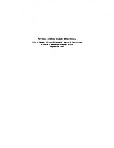
When building the relaxed temporal planning graph (RTPG), we ignored the negative interactions between concurrent actions. We now discuss a way of using the static mutex relations to help improve the heuristic estimation when extracting the relaxed plan. Specifically, our approach involves the following steps: 1. Find the set of static mutex relations between the ground actions in the planning problem based on their negative interactions. 2. When extracting the relaxed plan (Section 4.2), besides the orderings between actions that have causal-effect relationship (i.e one action gives the effect that supports the other action’s preconditions), we also establish the orderings according to the mutex relations. Specifically, when a new action is added to the relaxed plan, we use the pre-calculated static mutexes to establish ordering between mutually exclusive action pairs so that they can not be executed concurrently. The orderings are selected in such a way that they violate least number of existing causal links in the relaxed plan. By using the mutex relations, we can improve the makespan estimation of the relaxed plan, and thus the heuristic estimation. Moreover, in many cases, the mutex relations can also help us detect that the relaxed plan is in fact a valid plan, and thus can lead to the early termination of the search. Let’s take an example of the Logistics domain that is illustrated in Figure 6. In this example, we need to move two packages from cityA to cityB and cityC and there are two airplanes (plane1 , plane2 ) at cityA that can be used to move them. Moreover, we assume that plane1 is 1.5 times faster than plane2 and uses the same amount of resources to fly between two cities. There are two relaxed plans P1 = {move(package1 , plane1 , cityA, cityB), move(package2 , plane1 , cityA, cityC)} P2 = {move(package1 , plane1 , cityA, cityB), move(package2 , plane2 , cityA, cityC)} that both contain two actions. The first one has shorter makespan if mutexes are ignored. However, if we consider the mutex constraints, then we know that two actions in P1 can not be executed concurrently and thus the makespan of P1 is actually longer than P2 . Moreover, the static mutex relations also show that even if we order the two actions in P1 to be executed sequentially, there is a violation because the first action cuts off the causal link between the initial state and the second one. Thus, the mutex information helps us in this simple case to find a better quality (and consistent) relaxed plan to be used as a heuristic estimation. Here is a sketch of how the relaxed 18
plan P2 can be found. After the first action A1 = move(package1 , plane1 , cityA, cityB) is selected to support the goal at(package1 , cityB), the relaxed plan is RP = A1 and the two potential actions to support the second goal at(package2 , cityC) are A2 = move(package2 , plane1 , cityA, cityC) and A�2 = move(package2 , plane2 , cityA, cityC). With mutex information, we will be able to choose A�2 over A2 to include in the final relaxed plan. 4.2.2
Using the resource information to adjust the cost estimates
The heuristics discussed in the last two sections have used the knowledge about durations of actions and deadline goals but not resource consumption. By ignoring the resource related effects when building the relaxed plan, we may miss counting actions whose only purpose is to provide sufficient resource-related conditions to other actions.16 Consequently, ignoring resource constraints may reduce the quality of heuristic estimate based on the relaxed plan. We are thus interested in adjusting the heuristic values discussed in the last two sections to account for the resource constraints. In real-world problems, most actions consume resources, while there are special actions that increase the levels of resources. Since checking whether the level of a resource is sufficient for allowing the execution of an action is similar to checking the predicate preconditions, one obvious approach to adjust the relaxed plan would be to add actions that provide that resourcerelated condition to the relaxed plan. However, for many reasons, it turns out to be too difficult to decide which actions should be added to the relaxed plan to satisfy the given resource conditions (for a more elaborate discussion, see [9]). Therefore, we introduce an indirect way of readjusting the cost of the relaxed plan to take into account the resource constraints as follows: We first preprocess the problem specifications and find for each resource R an action AR that can increase the amount of R maximally. Let ∆R be the amount by which AR increases R, and let C(AR ) be the cost value of AR . Let Init(R) be the level of resource R at the state S for which we want to compute the relaxed plan, and Con(R), P ro(R) be the total consumption and production of R by all actions in the relaxed plan. If Con(R) > Init(R) + P ro(R), we use the following formula to adjust the cost component of the heuristic values according to the resource consumption: � � (Con(R) − (Init(R) + P ro(R))) � ∗ C(AR ) C←C+ ∆R R
We will call the newly adjusted heuristic adjusted cost. The basic idea is that even though we do not know if an individual resource-consuming action in the relaxed plan needs another action to support its resource-related preconditions, we can still adjust the number of actions in the relaxed plan by reasoning about the total resource consumption of all the actions in the plan. If we know how much excess amount of a resource R the relaxed plan consumes and what is the maximum increment of R that is allowed by any individual action in the domain, then we can infer the minimum number of resource-increasing actions that we need to add to the relaxed plan to balance the resource consumption. 16
In our ongoing example, if we want to drive a car from Tucson to LA and the gas level is low, by totally ignoring the resource related conditions, we will not realize that we need to refuel the car before drive it.
19
{Q}
{G} A1:
{G}
G
R
R
~R
S
A3:
T1
R
Q G
R S
T3
{Q}
A2:
R
Q
S ~R
A4:
T4
R S
T2
Figure 7: Examples of p.c. and o.c. plans
5 Post-processing to improve Temporal Flexibility To improve the makespan and execution flexibility of the plans generated by Sapa, we postprocess and convert them into partially ordered plans. We discuss the details of this process in this section. Position and Order constrained plans: A position constrained plan (p.c.) is a plan where the execution time of each action is fixed to a specific time point. An order constrained (o.c.) plan is a plan where only the relative orderings between the actions are specified. Sapa produces position constrained plans and the aim of post-processing is to convert them into order constrained ones. Figure 7 shows a valid parallel p.c. plan consisting of four actions A1 , A2 , A3 , A4 with their starting time points fixed to T1 , T2 , T3 , T4 and an o.c plan consisting of the same set of actions and achieving the same goals. For each action, the shaded regions show the durations in which each precondition or effect should hold during each action’s execution time. The darker ones represent the effect and the lighter ones represent preconditions. For example, action A1 has a precondition Q and effect R; action A3 has no precondition and two effects ¬R and S. The arrows show the relative orderings between actions. Those ordering relations represent the o.c plan and thus any execution trace that does not violate those orderings will be a consistent p.c plan. While generating a p.c. plan consistent with an o.c. plan is easy enough, we are interested in the reverse problem–that of generating an o.c. plan given a p.c. plan. Given a p.c plan Ppc , we discuss a strategy that finds a corresponding o.c plan Poc biased to have a reasonably good makespan. Specifically, we extend the explanation-based order generation method outlined in [23] to first compute a causal explanation for the p.c plan and then construct an o.c plan that has just the number of orderings needed to satisfy that explanation. This strategy depends heavily on the positions of all the actions in the original p.c. plan. Thus, it works based on the fact that the alignment of actions in the original p.c. plan guarantees that causation and preservation constraints are satisfied. To facilitate the discussion below, we use the following notations: • For each (pre)condition p of action A, we use [stpA , etpA ] to represent the duration in which p should hold (stpA = etpA if p is an instant precondition). • For each effect e of action A, we use eteA to represent the time point at which e occurs. • For each resource r that is checked for preconditions or used by some action A, we use [strA , etrA ] to represent the duration over which r is accessed by A. • The initial and goal states are represented by two new actions AI and AG . AI starts before 20
all other actions in the Ppc , it has no precondition and has effects representing the initial state. AG starts after all other actions in Ppc , has no effect, and has top-level goals as its preconditions. • The symbol �� ≺�� is used through out this section to denote the relative precedence orderings between two time points. Note that the values of stpA , etpA , eteA , strA , etrA are fixed in the p.c plan but are only partially ordered in the o.c plan. The o.c plan Poc is built from a p.c plan Ppc as follows: Supporting Actions: For each precondition p of action A, we choose action A� in the p.c plan to support p such that: 1. p ∈ Ef f ect(A� ) and etpA� < stpA in the p.c. plan Ppc . p 2. There is no action B such that: ¬p ∈ Ef f ect(B) and etpA� < et¬p B < stA in Ppc .
3. There is no other action C that also satisfies the two conditions above and etpC < etpA� . p
When A� is selected to support p to A, we add the causal link A� − → A between two time points etpA� and stpA to the o.c plan. Thus, the ordering etpA� ≺ stpA is added to Poc . Interference relations: For each pair of actions A, A� that interfere with each other, we order them as follows: � p ¬p 1. If ∃p ∈ Delete(A� ) Add(A), then add the ordering etpA ≺ et¬p A� to Poc if etA < stA� in ¬p p Ppc . Otherwise add etA� ≺ etA to Poc . � p 2. If ∃p ∈ Delete(A� ) P recond(A), then add the ordering etpA ≺ et¬p A� to Poc if etA < ¬p ¬p p etA in Ppc . Otherwise, if etA� < stA in the original plan Ppc then we add the ordering p et¬p A� ≺ stA to the final plan Poc . Resource relations: For each resource r that is checked as (pre)condition for action A and used by action A� , based on those action’s fixed starting times in the original p.c plan Ppc , we add the following orderings to the resulted Poc plan as follows: • If etrA < strA� in Ppc , then the ordering relation etrA ≺ strA� is added to Poc . • If etrA� < strA in Ppc , then the ordering relation etrA� ≺ strA is added to Poc . This strategy is backtrack-free due to the fact that the original p.c. plan is correct. All (pre)conditions of all actions in Ppc are satisfied and thus for any precondition p of an action A, we can always find an action A� that satisfies the three constraints listed above to support p. Moreover, one of the temporal constraints that lead to the consistent ordering between two interfered actions (logical or resource interference) will always be satisfied because the p.c. plan is consistent and no pair of interfered actions overlap each other in Ppc . Thus, the search is backtrack-free and we are guaranteed to find an o.c. plan due to the existence of one legal dispatch of the final o.c. plan Poc (which is the starting p.c. plan Ppc ). The final o.c. plan is valid because there is a causal-link for every action’s precondition, all causal links are safe, no interfering actions can overlap, and all the resource-related (pre)conditions are satisfied. Moreover, 21
this strategy ensures that the orderings on Poc are consistent with the original Ppc . Therefore, because the p.c plan Ppc is one among multiple p.c plans that are consistent with the o.c plan Poc , the makespan of Poc is guaranteed to be equal or better than the makespan of Ppc . The algorithm discussed in this section is a special case of the partialization problem in metric temporal planning. In [10], we do a systematic study of the general partialization problem and give CSOP (Constraint Satisfaction Optimization Problem) encodings for solving them. The current algorithm can be seen as a particular greedy variable/value ordering strategy for the CSOP encoding.
6 Implementation of Sapa Sapa system with all the techniques described in this paper has been fully implemented in JAVA. The search algorithm for metric temporal planning and other techniques have been incorporated in the current version. Specifically, they include: 1. The forward chaining algorithm (Section 2). 2. The cost sensitive temporal planning graph and the routines to propagate the cost information and extract the heuristic value from it (Section 3). 3. The routines to extract and adjust the relaxed plan with neglected mutex and resource information (Section 4.2). 4. Greedy post-processing routines to extract the causal structure between actions in the plan (Section 5). The default options for Sapa are sum-propagation rule, infinite lookahead termination, resourceadjusted heuristics, and solutions are greedily postprocessed. Beside the techniques described in this paper, we also wrote a JAVA-based parser for PDDL 2.1 Level 3, which is the highest level used in the Third International Planning Competition (IPC3). To visualize the plans returned by Sapa and the relations between actions in the plan (such as causal links, mutual exclusions, and resource relations), we have developed a Graphical User Interface (GUI)17 for Sapa. Figure 8 shows the screen shots of the current GUI. It displays the the time line of the final plan with each action shown with its actual duration and starting time in the final plan. There are options to display the causal relations between actions (found using the greedy approach discussed in Section 5), and logical and resource mutexes between actions. Annotations about the specific times at which individual goals are achieved are also displayed. Our implementation is publicly available through Sapa homepage (http://rakaposhi.eas.asu.edu/sapa.html). Given that the planer as well as the GUI are in JAVA, we also provide a web-based interactive access to the planner. 17
The GUI was developed by Dan Bryce
22
Figure 8: Screen Shots of Sapa’s GUI
6.1 Empirical evaluation We have subjected the individual components of the Sapa implementation to systematic empirical evaluation (c.f. [9, 11, 10]). In this section, we will describe the experiments that we conducted to show that Sapa [9] is capable of satisfying a variety of cost/makespan tradeoffs. Moreover, we also provide results to show the effectiveness of the heuristic adjustment techniques, the utility of different termination criteria, and the utility of the post-processing. The experiments in this section were run on the Unix SunBlade machine with 256MB of RAM. The evaluation of Sapa compared with other systems in the International Planning Competition, with data provided by the competition committee, are provided in the next section. Our first test suite for the experiments, which show the ability to produce solutions with tradeoffs between time and cost quality, consisted of a set of randomly generated temporal logistics problems provided by Haslum and Geffner [19]. In this set of problems, we need to move packages between locations in different cities. There are multiple ways to move packages, and each option has different time and cost requirements. Airplanes are used to move packages between airports in different cities. Moving by airplanes takes only 3.0 time units, but is expensive, and costs us 15.0 cost units. Moving packages by trucks between locations in different cities costs only 4.0 cost units, but takes longer time of 12.0 time units. We can also move packages between locations inside the same city (e.g. between offices and airports). Driving between locations in one city will cost us 2.0 units and takes 2.0 time units. Load/unload packages into truck or airplane takes 1.0 unit of time and cost 1.0 unit. We tested with the first 20 problems in the set with the objective function specified as a linear combination of both total execution cost and makespan values of the plan. Specifically, the objective function is set to O = α.C(P lan) + (1 − α).T (P lan) We tested with different values of α : 0 ≤ α ≤ 1. Among the techniques discussed in this paper, we used the sum-propagation rule, infinite look-ahead, and relax-plan extraction using static mutex relation. Figure 9 shows how the average cost and makespan values of the solution change according to the variation of the α value. The results show that the total execution cost of the solution decreases as we increase the α value (thus, giving more weight to the execution cost 23
Makespan Variation 31
50
29
Average solving time 50 40
30 20 10
time (secs)
27
40
Makespan
Total Cost
Cost variation 60
25 23 21 19
30 20 10
17
0
0
15
0.1
0.2
0.3
0.4
0.5
0.6
0
0.8
0.9
0.95
1
0.1
0.2
0.3
0.4
0.5
Alpha
0.6
0
0.8
0.9
0.95
0.1
1
0.2
0.3
0.4
0.5
0.6
0.7
0.8
0.9 0.95
1
Alpha
Alpha
Figure 9: Cost, makespan, and solving time variations according to different weights given to them in the objective function. Each point in the graph corresponds to an average value over 20 problems.
Relaxed Plan Prob
time(s)
node
#act
Relaxed Plan with Adjustment makespan
time(s)
node
#act
makespan
zeno1
0.272
14/48
5
320
0.317
14/48
5
320
zeno2
92.055
304/1951
23
1020
61.66
188/1303
23
950
zeno3
23.407
200/996
22
890
38.225
250/1221
13
430
zeno4
-
-
-
-
37.656
250/1221
13
430
zeno5
83.122
575/3451
20
640
71.759
494/2506
20
590
zeno6
64.286
659/3787
16
670
27.449
271/1291
15
590
zeno7
1.34
19/95
10
370
1.718
19/95
10
370
zeno8
1.11
27/87
8
320
1.383
27/87
8
320
zeno9
52.82
564/3033
14
560
16.310
151/793
13
590
log-p1
2.215
27/159
16
10.0
2.175
27/157
16
10.0
log-p2
165.350
199/1593
22
18.875
164.613
199/1592
22
18.875
log-p3
-
-
-
-
20.545
30/215
12
11.75
log-p4
13.631
21/144
12
7.125
12.837
21/133
12
7.125
log-p5
-
-
-
-
28.983
37/300
16
14.425
log-p6
-
-
-
-
37.300
47/366
21
18.55
log-p7
-
-
-
-
115.368
62/531
27
24.15
log-p8
-
-
-
-
470.356
76/788
27
19.9
log-p9
-
-
-
-
220.917
91/830
32
26.25
Table 1: Solution times, explored/generated nodes, number of actions, and makespan values of the solutions generated by Sapa in the zeno-flying and logistic domains with/without resource adjustment technique.
24
in the overall objective function). In contrast, when α decreases, thus giving more weight to the makespan, the final cost of the solution increases and the makespan value decreases. The results show that our approach indeed produces solutions that are sensitive to the objective functions that involve both time and cost. The right most graph in the Figure 9 shows the average solution time for this set of experiments. For all the combinations of {problem, α}, 79% (173/220) are solvable within our limit cutoff time of 300 seconds. The average solution time is 19.99 seconds and 78.61% of the instances can be solved within 10 seconds. The solid line shows the average solution time for different α values. The dashed line shows the average solving time if we take out the 20 (11%) combinations where the solving time is more than 40 seconds (more than two times the average value). We can see that while we generally have larger deviations, solving the multi-objective problems is not significantly costlier than single-objective problems (which corresponds to the end points of the plots). Utility of resource adjustment technique: In the second set of experiments, we test the utility of the resource adjustment technique discussed in Section 4.2.2 for heuristics discussed in Section 4. We evaluate the performance of Sapa on problems from two metric temporal planning domains. The first one is the zeno-flying domain discussed in [32]. The second is our version of the temporal and metric resource version of the logistics domain. In this domain, trucks move packages between locations within one city, and planes carry them from one city to another. Different airplanes and trucks move with different speeds, have different fuel capacities, different fuel-consumption-rates, and different fuel-fill-rates when refueling. The temporal logistics domain is more complicated than the zeno-flying domain because it has more types of resource-consuming actions. Moreover, the refuel action in this domain has a dynamic duration, which is not the case for any action in the zeno-flying domain. Specifically, the duration of this action depends on the fuel level of the vehicle and can only be decided at the time we execute that action. Table 1 shows the running times of Sapa for the relaxed-plan heuristic with and without metric resource constraint adjustment technique (refer to Section 4.2.2) in the two planning domains discussed above. We tested with 9 problems from each domain. Most of the problems require plans of 10-30 actions, which are quite big compared to problems solved by previous domain-independent temporal planners reported in the literature. The results show that most of the problems are solved within a reasonable time (e.g under 500 seconds). More importantly, the number of nodes (time-stamped states) explored, which is the main criterion used to decide how well a heuristic does in guiding the search, is quite small compared to the size of the problems. In many cases, the number of nodes explored by the best heuristic is only about 2-3 times the size of the plan. Table 1 also shows the number of actions in the solution and the duration (makespan) of the solutions. These categories can be seen as indicative of the problem’s difficulty, and the quality of the solutions. By closely examining the solutions returned, we found that the solutions returned by Sapa have quite good quality in the sense that they rarely have many irrelevant actions. The absence of irrelevant actions is critical in the metric temporal planners as it will both save resource consumption and reduce execution time. It is interesting to note here that the temporal TLPlan[1], whose search algorithm Sapa adapts, usually outputs plans with irrelevant actions. Interestingly, Bacchus & Ady mention that their solutions are still better than the ones
25
solving time (secs)
makespan
la ∞
la 0
0.15
0.16
320
38.40
0.78
-
0.31
0.38
650
0.32
0.36
-
9.05
2.99
670
0.27
0.33
330
333
0.27
0.24
zeno 8
177
0.17
zeno 9
216
0.21
log 1
424
log 2 log 3 log 4
4.28
log 5
-
log 6
2.43
log 7
3.64
log 8
6.53
log 9
3.60
cost la ∞
la 0
320
320
5
5
5
990
880
-
22
15
420
420
17
13
13
420
420
-
13
13
690
660
19
20
18
330
330
10
10
10
450
370
340
10
10
10
0.20
200
200
200
6
6
6
0.24
330
300
300
8
8
8
0.42
0.45
10
10
10
16
16
16
2.21
171.16
159.12
16.02
19.37
19.37
21
21
21
-
-
0.99
-
-
10.82
-
-
13
0.55
0.62
7.42
7.12
7.12
16
12
12
1.93
2.23
-
12.42
12.42
-
16
16
2.28
2.59
16.42
16.42
16.42
21
21
21
2.71
34.61
19.32
17.32
26.29
29
27
30
3.88
-
17.32
15.32
-
29
27
-
3.55
4.01
20.42
20.42
20.42
31
31
31
problem
la 0
zeno 1
157
zeno 2
-
zeno 3
1.69
zeno 4
-
zeno 5
3.25
zeno 6
238
zeno 7
la 1
la 1
la 1
la ∞
Table 2: Quality and solving time comparison for different termination criteria. returned by LPSAT[37], which makes our solutions that much more impressive compared to LPSAT. Evaluation of different termination criteria: For the same test suite discussed above (i.e. metric temporal zeno-flying and logistics domains), one and infinite lookahead options work similarly and are generally better than zero-lookahead. Table 2 shows the comparison results for zero, one, and infinite lookahead for the set of metric temporal planning problems discussed above. For the objective function, we set α = 1, actions costs are 1 unit and action durations are dependent on the distances between locations. In this test suite, the results show that while one and infinite lookahead work similar, they are generally better than zero-lookahead, both in term of solving time and solution quality. Utility of post-processing: Figure 10 shows the utility of the greedy post-processing technique discussed in Section 5. The test suite contains the same set of problems discussed earlier (i.e. random generated temporal logistics problem provided with TP4[19], and the metric temporal logistics problem). These graphs show the comparisons of makespan values of original parallel position-constrained (p.c) plans and the order-constrained (o.c) plans returned after post-processed. In the left side of Figure 10, we show the comparison between four different makespans for 20 largest problems among the 80 random temporal logistics problems provided 26
Logistics with Resources 120 30
100
25
20
Sum Dur
Makespan
makespan
80
Sapa's MS
60
After PP Opt. MS 40
20
Total Durs Sapa's MS
15
After PP 10
5
0
0
1
2
3
4
5
6
7
8
1
9 10 11 12 13 14 15 16 17 18 19 20
2
3
4
5
6
7
8
9
10
Problems
problems
Figure 10: Utility of the greedy post-processing approach for (left) random temporal logistics problem, and (right) metric temporal logistic problems. with TP4[19] planner. The makespan values are: (1) the optimal makespan (as returned by TGP [35]); (2) the makespan of the plan returned by Sapa; (3) the makespan of the o.c. resulting from the greedy algorithm for partialization discussed in the last section; and (4) the total duration of all actions, which would be the makespan value returned by several serial temporal planners such as AltAlt [29] or GRT [33] if they produce the same solution as Sapa. Notice that the makespan value of zero for the optimal makespan indicates that the problem is not solvable by TGP. Compared to the optimal makespan, on the average, the makespan of the serial p.c. plans (i.e, cumulative action duration) is about 4.34 times larger, the makespan of the plans output by Sapa is about 3.23 times larger and the Sapa plans after post processing are about 2.61 times longer (over the set of 75 solvable problems; TGP failed to solve the other 5). The graph on the right side of Figure 10 shows the utility of the greedy post-processing approach for the set of 10 metric temporal logistics problem discussed earlier in this section. Currently, there is no planner that can handle resources and output optimal makespan. Therefore, we compare only the total duration, the makespan of parallel plans output by Sapa, and the makespan values after partialization. The results show that on average, the backtrack-free value ordering strategy improves the makespan value by 22%.
6.2 Sapa in the 2002 International Planning Competition We entered an implementation of Sapa, using several of the techniques discussed in this paper, in the recent International Planning Competition. The specific techniques used in the competition version of Sapa are infinite look-ahead termination of cost propagation (Section 3.3), resource adjustment (Section 4.2.2), and greedy post-processing (Section 5). In the competition, we focused solely on the metric/temporal domains. Even though action cost is not part of the standard PDDL 2.1 language used in the competition, infinite-lookahead unit-cost propagation employed in Sapa helped it achieve very good performance in problems involving both metric and temporal constraints. The competition results were collected and distributed by the IPC3’s organizers and can be found at [13]. Detailed descriptions of domains used in the competition are also available at the same place.
27
The temporal planning domains in the competition come in two sets, one contains two domains Satellite and Rovers, provided by NASA, representing the applications investigated by them. Figures 11, 12, and 13 show the comparison results in the highest level of PDDL2.1 setting (in terms of the complexities of temporal and metric constraints involved) for the two domains Satellite and Rovers. Figure 11 and 12 show that five planners (Sapa, LPG, MIPS, TP4, and TPSYS) submitted results for the timed setting and only three (Sapa, MIPS, TP4) were able to handle the complex setting of the Satellite domain. In the timed setting, action durations depend on the setting of instruments aboard a particular satellite and the directions it needs to turn to. The “complex” setting is further complicated by the fact that each satellite has a different capacity limitation to store only a certain amount of image data. Goals involve taking images of different planets and stars located at different coordinate directions. To achieve the goals, the satellite equipped with the right set of equipment should turn to the right direction, calibrate and take the image. For the timed setting of this Satellite domain, Figure 11 shows that among five planners, Sapa, LPG and MIPS were able to solve 19 of 20 problems while TP4 and TPSYS were able to solve 2 and 3 problems respectively. For quality comparison, LPG with quality setting was able to return solutions with the best quality, Sapa was slightly better than LPG with speed setting and was much better than MIPS. LPG with speed setting is generally fastest, followed by MIPS and then Sapa and LPG with quality setting. For the complex setting, Figure 12 shows that, among the three planners, Sapa was able to solve the most number of problems (16), and generated plans with better quality than MIPS. TP4 produced the best quality solutions, but was able to solve only three smallest problems. The solving times of Sapa are slightly higher than MIPS, but are much better than TP4. The “timed” version of the Rover domain18 requires a set of scientific analysis to be done using a number of rovers. Each rover carries different set of equipment, and has a different energy capacity. Moreover, each rover can only recharge its battery at certain points (which may be unreachable) that are under the sun. Figure 13 shows that only Sapa and MIPS were able to handle the constraints involved with this problem set. Sapa again solved more problems (11 vs. 9) than MIPS and also returned better or equal quality solutions in all but one case. The solving time of MIPS is better than Sapa in 6 of 9 problems that it returns the solutions. In the second set of problems which come with temporal constraints, there are three domains: Depots, DriverLogistics and Zeno Travel. Sapa participated at the highest level, which is the “timed” settings for these three domains. Figure 14 shows the comparison between Sapa and three other planners (LPG, MIPS, and TP4) that submitted the results. In this domain, we need to move crates (packages) between different places, the loading actions that place the crates into each truck is complicated by the fact that they need an empty hoist. Thus, the Depot domain looks like a combination of the original logistics and blockworlds domains. Drive action durations depend on the distances between locations and the speed of the trucks, time for loading the crates depends on the power of the hoist that we use. There is no resource consumption in this highest level. In this domain, Sapa was only able to solve 5 problems, compared to 11 by MIPS and 18 by LPG. TP4 solved only one problem. For the problem that Sapa was able to solve, the 18
In the planning competition, each domain had multiple versions–depending on whether or not the actions had durations and whether actions use continuous resource.
28
Satellite-Time
Satellite-Time
700
1e+07 Sapa (19 solved) LPG (Quality) (19 solved) LPG (Speed) (19 solved) MIPS (Plain setting) (19 solved) TP4 (2 solved) TPSYS (3 solved)
600
Sapa (19 solved) LPG (Quality) (19 solved) LPG (Speed) (19 solved) MIPS (Plain setting) (19 solved) TP4 (2 solved) TPSYS (3 solved)
1e+06
500
Milliseconds
100000
Quality
400
300
10000
1000 200
100
100
0
10 0
2
4
6
8
10 12 Problem number
14
16
18
20
0
2
4
6
8
10 12 Problem number
14
16
18
20
Figure 11: Results for the time setting of the Satellite domain (from IPC3 results).
Satellite-Complex
Satellite-Complex
700
1e+07 Sapa (16 solved) MIPS (Plain setting) (10 solved) TP4 (3 solved)
Sapa (16 solved) MIPS (Plain setting) (10 solved) TP4 (3 solved)
600
1e+06
500
Milliseconds
100000
Quality
400
300
10000
1000 200
100
100
0
10 0
2
4
6
8
10
12
14
16
18
20
0
2
4
6
8
Problem number
10
12
14
16
18
20
Problem number
Figure 12: Results for the complex setting of the Satellite domain (from IPC3 results).
Rovers-Time
Rovers-Time
260
1e+06 Sapa (11 solved) MIPS (Plain setting) (9 solved)
240
Sapa (11 solved) MIPS (Plain setting) (9 solved)
220
100000
200
Milliseconds
Quality
180 160 140
10000
1000
120 100 100
80 60 40
10 0
2
4
6
8
10
12
14
16
0
Problem number
2
4
6
8
10
12
Problem number
Figure 13: Results for the time setting of the Rover domain (from IPC3 results).
29
14
16
Depots-Time
Depots-Time
1800
1e+07 Sapa (5 solved) LPG (Quality) (18 solved) LPG (Speed) (18 solved) MIPS (Plain setting) (11 solved) TP4 (1 solved)
1600
Sapa (5 solved) LPG (Quality) (18 solved) LPG (Speed) (18 solved) MIPS (Plain setting) (11 solved) TP4 (1 solved)
1e+06
1400 100000 Milliseconds
Quality
1200 1000 800 600
10000
1000
400 100 200 0
10 0
5
10
15
20
25
0
5
10
Problem number
15
20
25
Problem number
Figure 14: Results for the time setting of the Depots domain (from IPC3 results).
DriverLog-Time
DriverLog-Time
7000
1e+07 Sapa (14 solved) LPG (Quality) (20 solved) LPG (Speed) (20 solved) MIPS (Plain setting) (16 solved) TP4 (2 solved) TPSYS (1 solved)
6000
Sapa (14 solved) LPG (Quality) (20 solved) LPG (Speed) (20 solved) MIPS (Plain setting) (16 solved) TP4 (2 solved) TPSYS (1 solved)
1e+06
5000
Milliseconds
100000
Quality
4000
3000
10000
1000 2000
100
1000
0
10 0
2
4
6
8
10
12
14
16
18
20
0
2
4
6
8
Problem number
10
12
14
16
18
20
Problem number
Figure 15: Results for the time setting of the DriverLog domain (from IPC3 results).
ZenoTravel-Time
ZenoTravel-Time
1600
1e+06 Sapa (15 solved) LPG (Quality) (16 solved) LPG (Speed) (16 solved) MIPS (Plain setting) (20 solved)
1400
Sapa (15 solved) LPG (Quality) (16 solved) LPG (Speed) (16 solved) MIPS (Plain setting) (20 solved) 100000
1200
Milliseconds
Quality
1000
800
600
10000
1000
400 100 200
0
10 0
2
4
6
8
10
12
14
16
18
20
0
Problem number
2
4
6
8
10
12
14
16
18
Problem number
Figure 16: Results for the time setting of the ZenoTravel domain (from IPC3 results).
30
20
solution quality is as good as other planners. For the speed comparison, LPG with speed setting is clearly faster than other planners. Figure 15 shows how Sapa performance compares with other planners in the competition on the time setting of the DriveLog domain. This is a variation of the original Logistics domain in which we do not fly airplanes between different cities but only have to drive trucks between different locations. However, the driver needs to walk between different locations before he can board the truck. Like the Depot domain, there is no resource consumption. The durations for walking and driving depend on the specified time-to-walk and time-to-drive between them. In this domain, Sapa solved 14 problems compared to 20 by LPG, 16 by MIPS and 1 by TP4. The quality of the solutions by different planners are very similar. For the speed comparison, LPG with speed setting is fastest, then MIPS, then Sapa and LPG with quality setting. Finally, Figure 16 shows the performance of Sapa in the ZenoTravel domain with time setting. In this domain, passengers travel between different cities by airplanes. The airplanes can choose to fly with different speeds (fast/slow), which consuming different amount of fuel for each trip. Airplanes have different fuel capacity and need to refuel if they do not have enough in the tank for each trip. In this domain, Sapa and LPG solved 16 problems while MIPS solved 20. The solution quality of Sapa and MIPS are similar and in general better than LPG with either speed or quality setting. LPG with speed setting and MIPS solved problems in this domain faster than Sapa which in turn faster than LPG with quality setting. In summary, the competition results showed that Sapa is one of the best planners in IPC3 in solving problems involving both metric and temporal constraints.
7 Related Work and Discussion Although there have been several recent domain-independent heuristic planners aimed at temporal domains, most of them have been aimed at makespan optimization, ignoring the cost aspects. For example, both TGP [35] as well as TP4 [19] focus on makespan optimization and ignore the cost aspects of the plan. As we have argued in this paper, ultimately metric temporal planners have to deal with objective functions that are based on both makespan and cost. One recent research effort that recognizes the multi-objective nature of planning is Refanidis’ MO-GRT system [34]. On one hand, the MO-GRT approach is more general than our approach in the sense that it deals with the set of non-combinable quality metrics. MO-GRT approach however treats time similar to other consumable resources (with infinite capacity). Temporal constraints on the planning problems (such as when an effect should occur during the course of action), goal deadlines, or the concurrency between actions are ignored to scale down the problem to the classical planning assumptions. Like GRT, Metric-FF[22] and MIPS[12] are other forward state space planner that can handle resource constraints. Both of them generate sequential plan. MIPS can then handle durative actions by putting in the action duration and post-process the sequential p.c plans. Multi-Pegg [38] is another recent planner that considers cost-time tradeoffs in plan generation. Multi-Pegg is based on Graphplan approach, and focuses on classical planning problems with non-uniform cost actions. ASPEN [6] is another planner that recognizes the multi-attribute nature of plan quality. ASPEN advocates an iterative repair approach for planning, that assumes the availability of a variety of hand-coded plan repair strategies and their characterization in 31
terms of their effects on the various dimensions of plan quality. Along the lines of ASPEN, LPG[14] is another planner that employs the local search technique over the action-graph. LPG can handle objective functions that involve cost. Although we evaluated our cost-sensitive heuristics in the context of Sapa, a forward chaining planner, the heuristics themselves can also be used in other types of planning algorithms. For example, TGP can be made cost-sensitive by making it propagate the cost functions as part of planning graph expansion. These cost functions can then be used as a basis for variable and value ordering heuristics to guide its backward branch-and-bound search. A similar approach in classical planning has been shown to be successful in [24]. Besides Graphplan-based approaches, our framework can also be used in both forward and backward (state-space, and partial order planners (POP)) to guide the planning search. It is possible due to the fact that directional searches (forward/backward) all need to evaluate the distances between an initial state to the set of temporal goals. In classical planning, works by Nguyen & Kambhampati in [29, 30] have shown that heuristics derived from the classical planning graph can help guiding backward state space and partial order classical planners effectively. Even though the heuristics based on the level information in [29, 30] can not directly be extended to use in the temporal planning due to the fact that they assume all goals appear at the same time, our approach is more flexible and does not make such an assumption. The cost functions for facts and actions are based on the continuous time model and are independent of each other. Thus, they can be readily used in the backward planners, especially POP planners, where goals/subgoals are required at different time points. Our work is also related to other approaches that use planning graphs as the basis for deriving heuristic estimate such as Graphplan-HSP[24], AltAlt[29], RePOP[30], and FF[20]. In the context of these efforts, our contribution can be seen as providing a way to track cost as a function of time on planning graphs. An interesting observation is that cost propagation is in some ways inherently more complex than makespan propagation. For example, once a set of literals enter the planning graph (and are not mutually exclusive), the estimate of the makespan of the shortest plan for achieving them does not change as we continue to expand the planning graph. In contrast, the estimate of the cost of the cheapest plan for achieving them can change until the planning graph levels off. This is why we had to carefully consider the effect of different criteria for stopping the expansion of the planning graph on the accuracy of the cost estimates (Section 3.3). Another interesting observation is that within classical planning, there was often a confusion between the notions of cost and makespan. For example, the “length of a plan in terms of number of actions” can either be seen as a cost measure (if we assume that actions have unit costs), or a makespan measure (if we assume that the actions have unit durations). These notions get teased apart naturally in metric temporal domains. In this paper, we concentrated on developing heuristics that can be sensitive to multiple dimensions of plan quality (specifically, makespan and cost). An orthogonal issue in planning with multiple criteria, that we did not explicitly address here, is how the various dimensions of plan quality should be combined during optimization. The particular approach we adopted in our empirical evaluation–viz., considering a linear combination of cost and coverage–is by no means the only reasonable way. Other approaches involve non-linear combinations of the
32
quality criteria, as well as “tiered” objective functions (e.g. rank plans in terms of makespan, breaking ties using cost). A related issue is how to help the user decide the “weights” or “tiers” of the different criteria. Often the users may not be able to articulate their preferences between the various quality dimensions in terms of precise weights. A more standard approach out of this dilemma involves generating all non-dominated plans19 (the so-called “pareto-set” [7, 31]), and presenting them to the user (unfortunately, often the set of non-dominated plans can be exponential (c.f. [31])). The user is then expected to pick the plan that is most palatable to them. Further, the users may not actually be able to judge the relative desirability of plans when the problems are complex and the plans are long. Thus, a more practicable approach may involve resorting to other indirect methods such as preference elicitation techniques (c.f. [5]).
8 Conclusion In this paper, we presented Sapa, a domain-independent heuristic forward chaining planner that can handle durative actions, metric resource constraints, and deadline goals. Sapa is a forwardchaining planner that searches in the space of time-stamped states. It is designed to be capable of handling the multi-objective nature of the metric temporal planning. Our technical contributions included (i) a planning-graph based method for deriving heuristics that are sensitive to both cost and makespan (ii) an easy way of adjusting the heuristic estimates to take the metric resource limitations into account and (iii) a way of post-processing the solution plans to improve their execution flexibility. We described the technical details of extracting the heuristics and presented an empirical evaluation of the current implementation of Sapa. An implementation of Sapa using a subset of the techniques presented in this paper was one of the best domain independent planners for domains with metric and temporal constraints in the third International Planning Competition, held at AIPS-02. In the future, we intend to extend Sapa in several different directions. First, we want to make it more expressive in term of handling a richer set of temporal and resource constraints, such as exogenous events (e.g a rover can not recharge the battery after sunset). Another direction involves extending our multi-objective search to involve other quality metrics. While we considered cost of a plan in terms of a single monetary cost associated with each action, in more complex domains, the cost may be better defined as a vector comprising the different types of resource consumption. Further, in addition to cost and makespan, we may also be interested in other measures of plan quality such as robustness and execution flexibility of the plan. Our longer term goal is to support plan generation that is sensitive to these extended set of tradeoffs. To this end, we plan to extend our methodology to derive heuristics sensitive to a larger variety of quality measures. Finally, we also plan to consider the issues of planner-scheduler interactions in the context of Sapa. A plan P is said to be dominated by P � if the quality of P � is strictly superior to that of P in at least one dimension, and is better or equal in all other dimensions. 19
33
References [1] Bacchus, F. & Ady, M. 2001. Planning with Resources and Concurrency: A Forward Chaining Approach. In Proc. of Seventeenth International Joint Conference on Artificial Intelligence. [2] Backstrom, C. 1998. Computational Aspects of Reordering Plans. In Journal of Artificial Intelligence Research 9, 99-137. [3] Blum, A. and Furst, M. 1995. Fast planning throught planning graph analysis. In Proc. of Fourteenth International Joint Conference on Artificial Intelligence (IJCAI). [4] Bonet, B., Loerincs, G., and Geffner, H. 1997. A robust and fast action selection mechanism for planning. In Proc. of Fourteenth National Conference on Artificial Intelligence (AAAI) [5] U. Chajewska, L. Getoor, J. Norman and Y. Shahar. 1998. Utility Elicitation as a Classification Problem. In Proc. of Fourteenth Uncertainty in Artificial Intelligence Conference. [6] S. Chien, G. Rabideau, R. Knight, R. Sherwood, B. Engelhardt, D.Mutz, T. Estlin, B. Smith, F. Fisher, T. Barrett, G. Stebbins, D.Tran 2000. ASPEN - Automating Space Mission Operations using Automated Planning and Scheduling. In Proc. of SpaceOps-2000 [7] P. Dasgupta, P.P. Chakrabarti, and S.C. DeSarkar. Multiobjective Heuristic Search. Vieweg & Son/Morgan Kaufmann, 2001. [8] Dechter, R., Meiri, I., and Pearl, J. 1990. Temporal Constraint Network. In Artificial Intelligence Journal 49. [9] Do, M. and Kambhampati, S. 2001. Sapa: A domain independent heuristic metric temporal planner. In Proc. of Sixth European Conference on Planning [10] Do, M. and Kambhampati, S. 2002. Improving the Temporal Flexibility of Position Constrained Metric Temporal Planning. In Temporal Planning Workshop, AIPS-02 [11] Do, M., and Kambhampati, S. 2002. Planning graph-based heuristics for cost-sensitive temporal planning. In Proc. of Sixth International Conference on Artificial Intelligence Planning and Scheduling. [12] Edelkamp, S. 2001. First Solutions to PDDL+ Planning Problems In PlanSIG Workshop. [13] Fox, M. and Long, D. 2002. Third International Planning Competition. http://www.dur.ac.uk/d.p.long/competition.html [14] Gerevini, A. and Serina, I. 2002. LPG: A Planner Based on Local Search for Planning Graphs. In Proc. of Sixth International Conference on Artificial Planning and Scheduling (AIPS-02) [15] Long, D. and Fox, M. 1998 Efficient Implementation of the Plan Graph in STAN. In Journal of AI Research (JAIR), Volume 10, pages 87-115. 34
[16] Fox, M. and Long, D. 2001. PDDL2.1: An Extension to PDDL for Expressing Temporal Planning Domains. Technical Report. [17] Garrido, A., Onaindia, E., and Barber, F. 2001. Time-optimal planning in temporal problems. In Proc. of European Conference on Planning (ECP-01). [18] Ghallab, M. and Laruelle, H. 1994. Representation and control in IxTeT, a temporal planner. In Proc. of Second International Conference on Artificial Intelligence Planning and Scheduling [19] Haslum, P. and Geffner, H. 2001. Heuristic Planning with Time and Resources In Proc. of Sixth European Conference on Planning [20] Hoffmann, J. & Nebel, B. 2001. The FF Planning System: Fast Plan Generation through Heuristic Search. In Journal of Artificial Intelligence Research 14:253-302. [21] Hoffman, J. and Nebel, B. 2001. RIFO Revisited: Detecting Relaxed Irrelevance. In Proc. of 6th European Conference on Planning. [22] Hoffmann, J. 2002. Extending FF to Numerical State Variables. In Proc. of 15th European Conference on Artificial Intelligence. [23] Kambhampati, S. & Kedar, S. 1994. An unified framework for explanation-based generalization of partially ordered and partially instantiated plans. In Artificial Intelligence Journal 67, 29-70. [24] Kambhampati, S. and Nigenda, R. 2000. Distance based goal ordering heuristics for Graphplan. In Proc. of Fifth International Conference on Artificial Intelligence Planning and Scheduling. [25] Koehler, J. 1998. Planning under Resource Constraints. In Proc. of Eleventh European Conference on Artificial Intelligence [26] J. Koehler, B. Nebel, J. Hoffmann, Y. Dimopoulos. Extending Planning Graphs to an ADL Subset In Proc. of European Conference in Planning. [27] Laborie, P. and Ghallab, M. Planning with sharable resource constraints. In Proc. of Fourteenth International Joint Conference on Artificial Intelligence (IJCAI). [28] Muscettola, N. 1994. Integrating planning and scheduling. Intelligent Scheduling. [29] Nguyen, X., Kambhampati, S., and Nigenda, R. 2001. Planning Graph as the Basis for deriving Heuristics for Plan Synthesis by State Space and CSP Search. In Artificial Intelligence Journal. [30] Nguyen, X., and Kambhampati, S., 2001. Reviving Partial Order Plan In Proc. of Seventeenth International Joint Conference on Artificial Intelligence (IJCAI).
35
[31] Papadimitriou C. H. and Yannakakis M. Multiobjective Qury Optimization. ACM Conference on Principles of Database Systems (PODS) 2001. [32] Penberthy, S. and Well, D. 1994. Temporal Planning with Continuous Change. In Proc. of 11th National Conference on Artificial Intelligence (AAAI). [33] Refanidis, I. and Vlahavas, I. 2001. The GRT Planner: Backward Heuristic Construction in Forward State Space Planning. Journal of Artificial Intelligence Research, 15.p:115-161. [34] Refanidis, I. and Vlahavas, I. 2001. A Framework for Multi-Criteria Plan Evaluation in Heuristic State-Space Planning Workshop on Planning with Resources, IJCAI-01. [35] Smith, D. and Weld, D. 1999. Temporal Planning with Mutual Exclusion Reasoning. In Proc. of 16th International Joint Conference on Artificial Intelligence (IJCAI) [36] Tsamardinos, I., Muscettola, N. and Morris, P. Fast Transformation of Temporal Plans for Efficient Execution. In Proc. 15th National Conference on Artificial Intelligence (AAAI). [37] Wolfman, S. and Weld, D. 1999. The LPSAT system and its Application to Resource Planning. In Proc. of 16th International Joint Conference on Artificial Intelligence. [38] Zimmerman, T. 2002. Generating parallel plans satisfying multiple criteria in anytime fashion. In Workshop on Planning and Scheduling with Multiple criteria, AIPS-2002
36