the notion of optimally reachable belief spaces to improve com- putational .... It is known that V â, the value function associated with the optimal policy Ïâ, can ...
IN
Proc. Robotics: Science & Systems, 2008
SARSOP: Efficient Point-Based POMDP Planning by Approximating Optimally Reachable Belief Spaces Hanna Kurniawati
David Hsu
Wee Sun Lee
Department of Computer Science, National University of Singapore Singapore 117590, Singapore Abstract— Motion planning in uncertain and dynamic environments is an essential capability for autonomous robots. Partially observable Markov decision processes (POMDPs) provide a principled mathematical framework for solving such problems, but they are often avoided in robotics due to high computational complexity. Our goal is to create practical POMDP algorithms and software for common robotic tasks. To this end, we have developed a new point-based POMDP algorithm that exploits the notion of optimally reachable belief spaces to improve computational efficiency. In simulation, we successfully applied the algorithm to a set of common robotic tasks, including instances of coastal navigation, grasping, mobile robot exploration, and target tracking, all modeled as POMDPs with a large number of states. In most of the instances studied, our algorithm substantially outperformed one of the fastest existing point-based algorithms. A software package implementing our algorithm will soon be released at http://motion.comp.nus.edu.sg/ projects/pomdp/pomdp.html.
I. I NTRODUCTION Partially observable Markov decision processes (POMDPs) [17] provide a principled mathematical framework for planning under uncertainty, an essential capability for robots operating in uncertain and dynamic environments. However, POMDPs are often avoided in robotics, because solving POMDPs exactly is computationally intractable [9]. Not long ago, the best algorithms could spend hours computing exact solutions to POMDPs with only a dozen states, which are woefully inadequate for modeling realistic robotic tasks. In recent years, point-based POMDP algorithms [5, 10, 16, 19, 20] have made impressive progress by computing good approximate solutions: POMDPs with hundreds of states have been solved in a matter of seconds (e.g., [5, 16, 19]). These algorithms have the potential to make POMDPs practical for many applications in robotics and beyond. Our goal is to create practical POMDP algorithms and software for common robotic tasks. To this end, we have developed a new point-based POMDP algorithm that exploits the notion of optimally reachable belief spaces to improve computational efficiency. In simulation, we successfully applied our algorithm to a set of common robotic tasks, including coastal navigation, grasping, mobile robot exploration, and target tracking, all modeled as POMDPs with a large number of states. POMDP algorithms typically operate in a robot’s belief space. A belief is a probability distribution over all possible robot states, and the set of all beliefs form the belief space. Intuitively, the difficulty of solving POMDPs is due to the “curse of dimensionality”: in a discrete POMDP, the belief space B has dimensionality equal to |S|, the number of robot
B R(b0 ) b0
R∗ (b0 )
Fig. 1. Belief space B, reachable space R(b0 ), and optimally reachable space R∗ (b0 ). Note that R∗ (b0 ) ⊆ R(b0 ) ⊆ B.
states. The size of B thus grows exponentially with |S|. Consider, for example, robot navigation in a simple planar environment modeled as a 10 × 10 grid. The resulting belief space is 100-dimensional! To overcome this difficulty, one key idea of point-based POMDP algorithms is to sample a set of points from B and use it as an approximate representation of B, instead of representing B exactly. Some early POMDP algorithms sample the entire belief space B, using a uniform sampling distribution, such as a grid. However, it is difficult to sample a representative set of points from B, due to its large size. More recent point-based algorithms sample only R(b0 ), the subset of belief points reachable from a given initial point b0 ∈ B, under arbitrary sequences of actions (Fig. 1). It is generally believed that R(b0 ) is much smaller than B. Indeed, focusing on R(b0 ) allows point-based algorithms to scale up to larger problems. To push further in this direction, we would like to sample near R∗ (b0 ), the subset of belief points reachable from b0 under optimal sequences of actions, as R∗ (b0 ) is usually much smaller than R(b0 ). Of course, the optimal sequences of actions constitute exactly the POMDP solution, which is unknown in advance. In fact, knowing R∗ (b0 ) is in some sense “equivalent” to knowing the POMDP solution (see Section IIIA). So we need to approximate R∗ (b0 ). The main idea of our algorithm is to compute successive approximations of R∗ (b0 ) and converge to it iteratively. Since R∗ (b0 ) is unknown in advance, the algorithm relies on heuristic exploration to sample R(b0 ) and improves sampling over time through a simple on-line learning technique. It then uses a bounding technique to avoid sampling in regions that are unlikely to be optimal and focus sampling on the region near R∗ (b0 ), the subset of B most relevant to the POMDP solution. This leads to substantial gain in computational efficiency. Focusing on R∗ (b0 ) also brings an indirect benefit. Under fairly general conditions, the solution to a POMDP can be represented as a convex, piecewise-linear value function [17].
We represent the value function as a set Γ of hyperplanes, each of which must dominate the rest at some sampled point. By pruning away sampled points that are suboptimal, i.e., outside R∗ (b0 ), we can reduce the size of Γ, thus further improving computational efficiency. II. BACKGROUND A. POMDPs A POMDP models an agent taking a sequence of actions under uncertainty to maximize its reward. Formally it is specified as a tuple (S, A, O, T , Z, R, γ), where S is a set of states, A is a set of actions, and O is a set of observations. In each time step, the agent lies in some state s ∈ S; it takes some action a ∈ A and moves from s to a new state s0 . Due to the uncertainty in action, the end state s0 is modeled as a conditional probability function T (s, a, s0 ) = p(s0 |s, a), which gives the probability that the agent lies in s0 , after taking action a in state s. The agent then makes an observation to gather information on its state. Due to the uncertainty in observation, the observation result o ∈ O is again modeled as a conditional probability function Z(s, a, o) = p(o|s, a). In each step, the agent receives a real-valued reward R(s, a), if it takes action a in state s, and the goal of the agent is to maximize its expected total reward by choosing a suitable sequence of actions. For infinite-horizon POMDPs, the sequence of actions has infinite length. We specify a discount factor γ ∈ [0, 1) so that the total reward is finite and the problem is well defined. P∞ In this case, the expected total reward is given by E [ t=0 γ t R(st , at )], where st and at denote the agent’s state and action at time t. The solution to a POMDP is an optimal policy that maximizes the expected total reward. Normally, a policy is a mapping from the agent’s state to a prescribed action. However, in a POMDP, the agent’s state is partially observable and not known exactly. So we rely on the concept of beliefs. As described earlier, a belief is a probability distribution over S. A POMDP policy π: B → A maps a belief b ∈ B to a prescribed action a ∈ A. A policy π induces a value function V π (b) that specifies the expected total reward of executing policy π starting from b. It is known that V ∗ , the value function associated with the optimal policy π ∗ , can be approximated arbitrarily closely by a convex, piecewise-linear function V (b) = max(α · b), α∈Γ
where Γ is a finite set of vectors called α-vectors, b is the discrete vector representation of a belief, and α · b is the inner product of vectors α-vector and b. Each α-vector is associated with an action. The policy can be executed by selecting the action corresponding to the best α-vector at the current belief. So a policy can be represented as a set of α-vectors. B. Related Work POMDPs are a principled approach for planning and decision making under uncertainty [6, 17], but they are notoriously hard to solve [7, 9]. There have been significant efforts in
developing approximation algorithms. See [1] for a recent survey. Point-based algorithms have been particularly successful in computing approximate solutions to large POMDPs [2, 5, 10, 16, 19, 20]. Most of them use value iteration [13]. Exploiting the fact that the optimal value function must satisfy the Bellman equation [13], value iteration algorithms start with an initial policy represented as a value function V and perform backup operations on V by iterating on the Bellman equation until the iteration converges. One important idea shared by the point-based algorithms is to sample a representative set of points from the belief space B and compute an approximately optimal value function by performing backup operations over the sampled points rather than the entire B. They differ in how they sample the belief space and perform backup operations. To improve computational efficiency, recent pointbased algorithms sample only the reachable space R(b0 ) from an initial belief point b0 . PBVI [10] is the first point-based algorithm that demonstrated good performance on a large POMDP called Tag, which has 870 states. Later point-based algorithms improved the performance significantly on this and other larger POMDPs. To our knowledge, HSVI2 [19] so far has the best performance in general. HSVI2 uses heuristics to guide the sampling towards regions that help cut down the gap between the upper and lower bounds on the optimal value function. FSVI [16] is another point-based algorithm, which uses a Markov decision process (MDP) to guide the sampling. MDP-guided sampling is effective for some problems, but the performance degrades when uncertainty is high and long sequences of information-gathering actions are required. Our algorithm is related to HSVI2 and FSVI, but it explicitly attempts to sample the optimally reachable space R∗ (b0 ) through learning-enhanced exploration and a bounding technique. Experimental results show that focusing on R∗ (b0 ) is a promising idea. An early version of our algorithm [5] exploits bounding in a limited way: bounds are compared locally at individual belief points to prune suboptimal actions. In contrast, the current algorithm sets up the bounds to reach a specified value function approximation level at b0 , thereby leveraging information globally to reduce the number of poor samples—those that are in R(b0 ) but not in R∗ (b0 ). One crucial reason for the computational intractability of POMDPs is the high dimensionality of B. Low-dimensional approximations of B therefore improve computational efficiency greatly (e.g., [12, 14]). These approaches are important, but beyond the scope of this paper. III. SARSOP We now describe our algorithm, SARSOP, which stands for Successive Approximations of the Reachable Space under Optimal Policies. A. Optimally Reachable Spaces A key idea of point-based POMDP algorithms is to sample a representative set of points from the belief space and
Algorithm 1 SARSOP. 1: Initialize the set Γ of α-vectors, representing the lower bound V on the optimal value function V ∗ . Initialize the upper bound V on V ∗ . 2: Insert the initial belief point b0 as the root of the tree TR . 3: repeat 4: SAMPLE (TR , Γ). 5: Choose a subset of nodes from TR . For each chosen node b, BACKUP(TR , Γ, b). 6: PRUNE (TR , Γ). 7: until termination conditions are satisfied. 8: return Γ. use it as an approximate representation of the space. For efficiency, most recent algorithms sample from R(b0 ), the set of points reachable from a given point b0 ∈ B under arbitrary sequences of actions. Theoretical analysis shows that approximate POMDPs solutions can be computed efficiently, when R(b0 ) has a small covering number [4]. Informally, the δ-covering number C(δ) of a set S is the minimum number of balls of radius δ needed to cover S. So it is a measure of the “volume” of S. Theorem 1: For any b0 ∈ B, let C(δ) be the δ-covering number of R(b0 ). Given any constant � > 0, an approximation V (b0 ) of V ∗ (b0 ), with error |V ∗ (b0 ) − V (b0 )| ≤ �, can be found in time ! �2 � (1 − γ)� (1 − γ)2 � . logγ O C 4γRmax 2Rmax However, for many realistic robotics tasks, the assumption of small R(b0 ) may not hold. We would like our algorithm to do well when R(b0 ) may be large, but Rπ∗ (b0 ), the space reachable under an optimal policy π ∗ , is small. As Rπ∗ (b0 ) is often much smaller than R(b0 ), the assumption of small Rπ∗ (b0 ) is more likely to hold. Unfortunately, this relaxed assumption is too weak, and the problem of computing approximate POMDP solutions remains hard, despite the assumption [4]. Theorem 2: Let b0 be any point in B and π ∗ be an optimal policy. Given a constant � > 0, computing an approximation V (b0 ) of V ∗ (b0 ), with error |V (b0 ) − V ∗ (b0 )| ≤ �|V ∗ (b0 )|, is NP-hard, even if the covering number of Rπ∗ (b0 ) is polynomial-sized. On the other hand, if we are given a set of balls of radius δ that covers Rπ∗ (b0 ), the problem becomes much easier [4]. We call the set C, which contains the centers of this set of balls, a δ-cover of Rπ∗ (b0 ). Theorem 3: For any b0 ∈ B and any optimal policy π ∗ , 2 � given a proper δ-cover C of Rπ∗ (b0 ) with δ = (1−γ) 2γRmax , an ∗ ∗ approximation V (b0 ) of V (b0 ), with error |V (b0 )−V (b0 )| ≤ �, can be found in time � � (1 − γ)� 2 , O |C| + |C| logγ 2Rmax where |C| is the size of C and Rmax = maxs,a |R(s, a)| is the maximum one-step reward.
b0 a1 a 2
o1 o2
Fig. 2.
The belief tree TR rooted at b0 .
Together, Theorems 2 and 3 say that computing approximate POMDP solutions is hard, but the problem becomes much easier, if a proper δ-cover of Rπ∗ (b0 ) is given. It follows that the key difficulty must lie in computing such a cover. Once the cover is obtained, we can find an approximate POMDP solution in time polynomial in the cover size. So, instead of following the common approaches of directly approximating V ∗ or searching for π ∗ , our SARSOP algorithm focuses on finding an approximate cover of Rπ∗ (b0 ) through sampling. Since there may beS multiple optimal policies, SARSOP aims to sample R∗ (b0 ) = π∗ Rπ∗ (b0 ), the union of all optimally reachable spaces. In the following, to simplify the notations, we omit the argument b0 in R(b0 ) and R∗ (b0 ). It is understood that R and R∗ are reachable from a given initial point b0 . B. Overview of the Algorithm SARSOP iterates over three main functions, SAMPLE, and PRUNE. A sketch is shown in Algorithm 1. Like all point-based algorithm, SARSOP samples a set of points from the belief space. The sampled points form a tree TR (Fig. 2). Each node of TR represents a sampled point. As there is no confusion, we use the same symbol b to denote both a sampled point and its corresponding node in TR . The root of TR is the initial belief point b0 . To sample a new point b0 , we pick a node b from TR as well as an action a ∈ A and an observation o ∈ O according to suitable probability distributions or heuristics. We then compute b0 using the formula X b0 (s0 ) = τ (b, a, o) = ηZ(s0 , a, o) T (s, a, s0 )b(s), BACKUP ,
s
where η is a normalization constant, and insert b0 into TR as a child of b. Clearly, every point sampled this way is reachable from b0 . If we apply all possible sequences of actions and observations, the set of nodes in TR is exactly R. The key is, of course, to avoid doing so and focus the sampling, instead, on R∗ . To achieve this, SARSOP maintains both a lower bound V and an upper bound V on the optimal value function V ∗ . The set Γ of α-vectors represents a piecewise-linear approximation to V ∗ (Section II-A), and is also a lower bound when suitably initialized, using, e.g., a fixed-action policy [1]. For the upper bound V , SARSOP uses the sawtooth approximation [1]. The upper bound can be initialized in various ways, using the MDP or the Fast Informed Bound technique [1]. SARSOP uses the
Algorithm 2 Perform α-vector backup at a node b of TR . BACKUP(TR , Γ, b) 1: For all a ∈ A, o ∈ O, αa,o ← argmaxα∈Γ (α · τ (b, a, o)). 2: For all a ∈ A, s ∈ S, P αa (s) ← R(s, a) + γ o,s0 T (s, a, s0 )Z(s0 , a, o)αa,o (s0 ). 3: α0 ← argmaxa∈A (αa · b) 4: Insert α0 into Γ. upper and the lower bounds to bias sampling towards R∗ ( (see Section III-C). Next, we perform backup at selected nodes in TR . A backup operation at a node b collates the information in the children of b and propagates it back to b. We perform the standard αvector backup (Algorithm 2), with the value function approximation represented as a set Γ of α-vectors. The value function approximation at b, obtained from the α-vector backup, is the same as that from the Bellman backup. However, the Bellman backup propagates only the value, while the α-vector backup propagates the gradient of the value function approximation along with the value to obtain a global approximation over the entire belief space rather than a local approximation at b. Invocation of SAMPLE and BACKUP generates new sampled points and α-vectors. However, not all of them are useful for constructing an optimal policy and are pruned to improve computational efficiency (see Section III-D). SARSOP is an anytime algorithm that returns the best policy found within a pre-specified amount of time. It gradually reduces the gap � between the upper and lower bounds on the value function at b0 , until it reaches either a pre-specified gap size or the time limit. C. Sampling The NP-hardness result described in Section III-A suggests that sampling from R∗ is hard. We use heuristics and information gathered from earlier samples to guide the sampling and improve the sampling distribution over time. Furthermore, by using value function bounds, we try to avoid sampling in regions that are unlikely to be reachable under any optimal policy, i.e., outside of R∗ . See Algorithm 3 for the pseudocode. To sample new belief points, SARSOP sets a target gap size � between the upper and lower bound at the root b0 of TR and traverses a single path down TR by choosing at each node the action with the highest upper bound and the observation that makes the largest contribution to the gap at the root of TR . This is the same action and observation selection strategy used in HSVI2 [19]. The sampling path is terminated under suitable conditions. Together, the strategies for action and observation selection and the choice of termination conditions control the resulting sampling distribution. One termination condition is to stop when the sampling path reaches a node whose gap between the upper and lower bounds is smaller than γ −t �, where t is the depth of the node in TR [19]. If each leaf of TR has a gap smaller than γ −t �, the gap at the root is guaranteed to be smaller than �. This condition, although reasonable, is inadequate. As the target gap � at the root gets smaller, the sampling path must traverse
deeper down the tree. As we go down the tree, the set of points in R increases much faster than the set of points in R∗ , and it becomes increasingly difficult to sample from R∗ . To focus sampling near R∗ and minimize sampling in R\R∗ , we would like to make the sampling path as shallow as possible while still achieving the target gap � at the root of TR . A potential dilemma here is that some nodes with high expected rewards lie deep in the tree, and we must allow the sampling path to go deep enough in order to reach them. a) Selective deep sampling: As each backup operation chooses the action that maximizes the expected reward, improvements in lower bounds are quickly propagated to the root when nodes with high expected rewards are found. This not only directly improves the policy but also provides information to stop sampling more quickly in regions that are likely outside R∗ . In contrast, upper bounds cannot be propagated beyond a node until the upper bounds for all the actions at the node are sufficiently improved. Finding the best action is not enough. Thus we give preference to lower bound improvements and continue down a sampling path beyond the node with a gap of γ −t �, if we predict that doing so likely leads to improvement in the lower bound at the root. To make such a predication, conceptually we predict the optimum value V ∗ (b) at a node b and propagate the predicted value Vˆ up towards the root. If Vˆ improves the lower bound at the root, we expand b and then repeat the procedure at the next selected node down the sampling path. Otherwise, we proceed to check the gap termination criterion described in the next subsection. To predict the optimal value V ∗ (b), we use a simple learning technique. We cluster beliefs according to suitable features and use previously computed values of beliefs in the same cluster as b to predict the value of b. This allows us to learn which parts of the belief space is worth exploring. Currently, we use the initial upper bound and the entropy of b as the features and discretize the belief space into a finite number of bins according to these two features. The average value of beliefs in a bin is used as the prediction for the value of any new belief falling into the bin. If a bin is empty, the initial upper bound of the new belief is used as its predicted value. To implement this idea efficiently, we do not actually propagate the predicted value Vˆ back to the root. Instead, we pass a lower-bound target level L down the sampling path. The predicted value Vˆ is checked against L. If Vˆ fails to meet the target L at a node b, the lower bound at b will not be propagated further up towards the root of TR . Let us now consider how to pass the target L at a node b to a child node b0 = τ (b, a, o). First, observe that value function information is propagated up from b0 to b only if the action a that takes b to b0 has higher value than all other actions at b. We thus calculate an intermediate target level L0 for a, which is set to the maximum over L and the values of all the actions at b (Algorithm 3, lines 7–8). Next, observe that the lower bound on the value of action a is X X R(s, a)b(s) + γ p(o|b, a)V (b0 ). Q(b, a) = s
o
Algorithm 3 Sampling near R∗ . S AMPLE(TR , Γ) 1: Set L to the current lower bound on the value function at the root b0 of TR . Set U to L + �, where � is the current target gap size at b0 . 2: S AMPLE P OINTS (TR , Γ, b0 , L, U , �, 1). S AMPLE P OINTS(TR , Γ, b, L, U , �, t). ˆ be the predicted value of V ∗ (b). 3: Let V ˆ 4: if V ≤ L and V (b) ≤ max{U, V (b) + �γ −t } then 5: return 6: else 7: Q ← maxa Q(b, a). 8: L0 ← max{L, Q}. 9: U 0 ← max{U, Q + γ −t �}. 10: 11: 12:
13:
14: 15: 16:
a0 ← arg maxa Q(b, a). o0 ← arg maxo p(o|b, a0 ) V (τ (b, a0 , o))− V (τ (b, a0 , o))). P 0 Calculate Lt so that L0 = s R(s, a )b(s) � � + P 0 0 0 0 γ p(o |b, a )Lt + o6=o0 p(o|b, a )V (τ (b, a , o)) . P 0 Calculate Ut so that U 0 = s R(s, a )b(s) � + � P 0 0 0 0 γ p(o |b, a )Ut + o6=o0 p(o|b, a )V (τ (b, a , o)) . b0 ← τ (b, a0 , o0 ). Insert b0 into TR as a child of b. S AMPLE P OINTS (TR , Γ, b0 , Lt , Ut , �, t + 1).
Hence the target level for b0 is the value needed for Q(b, a) to achieve its target L0 (Algorithm 3, line 12). To guard against misleading predictions that result in unnecessarily deep samplings paths, we only continue down a sampling path until the gap between the upper and lower bounds is κγ −t � for some κ < 1. The κ value is set to 0.5 in our current implementation. b) The gap termination criterion: If our prediction shows no improvement of the lower bound at the root, we use the target gap size � at the root to decide whether to terminate the sampling path and avoid sampling in regions unlikely to be in R∗ . As mentioned earlier, the straightforward way of achieving the target gap size � between the upper and lower bounds at the root of TR is to require a gap size γ −t � for all leaves of TR . However, it is in fact sufficient to ensure that the condition is satisfied somewhere along all the paths from the root to the leaves, rather than at the leaves themselves. This has the advantage of leveraging information globally from the other parts of TR to terminate a sampling path as early as possible and thus improving computational efficiency. To do this, we pass an upper-bound target level U down the sampling path as well. For a node b at depth t, we can terminate sampling if its upper bound is lower than V (b) + �γ −t or the upper-bound target U passed down from parent of b. This termination criterion has the same effect as requiring all leaves to have a gap of no more than �γ −t : if all leaves in TR meet this termination criterion, the root b0 achieves the
target gap size of �. The upper-bound target level U can be passed down a sampling path in a way similar to that for the lower-bound target level L. See Algorithm 3, lines 9 and 13. The combination of selective deep sampling and the gap termination criterion leads to an effective sampling strategy that goes deep into TR when need. This avoids unnecessarily sampling in R\R∗ and gives a better approximation to R∗ . D. Pruning The efficiency of backup operations, which take up a significant fraction of the total computation time, depends significantly on the size of the set Γ of α-vectors. To improve computational efficiency, existing point-based algorithms usually prune an α-vector from Γ if it is dominated by others over the entire belief space B. The notion of optimally reachable space suggests an alternative and more aggressive pruning technique: ideally, we want to prune an α-vector if it is dominated by other α-vectors over R∗ , rather than B. Since R∗ is potentially much smaller than B, this may substantially reduce the size of Γ and improve the efficiency of the backup operations and thus the overall algorithm. As R∗ is not known in advance, we use B, the set of all sampled belief points contained in TR , as an approximation. To improve this approximation and to keep the size of B small, we prune from B those points that are provably suboptimal and do not lie in R∗ . For a node b in TR , if Q(b, a) < Q(b, a0 ) for two actions a and a0 , then we prune all the sampled points in the subtree resulting from taking action a at b, as an optimal policy will never take the action a at b and traverse the subtree underneath. It is possible that some pruned points may turn out to lie in R∗ , as there are other paths in TR to reach them under an optimal policy. However, the benefits of keeping B small usually outweighs the loss in the approximation quality due to over-pruning. These points can also be eventually recovered from the other paths in TR . Belief point pruning in turn enables more aggressive αvector pruning. In SARSOP, an α-vector is pruned if it is dominated by others over B. A simple criterion for dominance is to say that for two α-vectors α1 and α2 , α1 dominates α2 at a belief point b if α1 · b ≥ α2 · b. However, this is not robust. The set B is a finitely sampled approximation of R∗ . Since SARSOP computes an approximately optimal policy over B only, the computed policy may choose an action that causes it to slightly veer off R∗ and get into a region in which the value function approximation is poor. To address this issue, we impose the more stringent requirement of dominance over a δneighborhood: α1 dominates α2 at a belief point b if α1 · b0 ≥ α2 · b0 at every point b0 whose distance to b is less than δ, for some fixed constant δ. We call this δ-dominance. We can check δ-dominance very quickly by computing the distance d from b to the intersection of the hyperplanes represented by α1 and α2 and making sure that d ≥ δ. In the implementation, the value of δ can be set adaptively according to the effectiveness of α-vector pruning. A similar idea for α-vector pruning, but without using the δ-neighborhood, is described in [15].
(a) Underwater Navigation, an instance of coastal navigation, shown on a reduced map with a 11 × 12 grid. “S” marks the possible initial positions for the robot. The robot is equally likely to start in any of these positions. “D” marks the destinations. “R” marks the rocks. “O” marks places that the robot can fully localize itself.
(b) Grasping. A fingered robot arm grasps a stepped block. Courtesy of L.P. Kaelbling and T. Lozano-P´erez.
(c) Integrated Exploration. A robot navigates with an uncertain map. Areas shaded in black represent obstacles. Areas shaded in light gray represent (possibly damaged) bridges. “S” marks the start location for the robot. “D” marks destination locations. bathroom
target
robot
Fig. 3.
(d) Homecare. A robot follows a moving person, the target. The light blue areas indicate obstacles. The black dashed curve indicates the target’s path. The green area around the robot indicates the the robot sensor’ visibility region. The various shades of gray show the robot’s belief of the current target position.
Some common robotic tasks modeled as POMDPs.
IV. E XPERIMENTS We have successfully applied SARSOP to a set of distinct robotic tasks. In this section, we describe these tasks, the experimental setup, and the results. A. Robotic Tasks Studied Uncertainty arises in various ways in robotic systems. Suppose that the state of a robotic system is given by (xr , xe ), where xr represents the state of the robot and xe represents the state of the environment. Inaccuracies in robot control and sensing are the typical causes for uncertainty in xr . They are
almost always present to some degree. Uncertainty in xe , On the other hand, varies widely. We thus divide the robotic tasks studied here into three categories according to the uncertainty in xe . In the first category, the environment is static and known with high accuracy. So uncertainty in xe can be ignored, and we only need to consider uncertainty in xr in planning the robot’s actions. In the second category, the environment is static, but not known accurately. Thus, we must take into account the uncertainty in both xr and xe in planning. In the last category, the environment is not static and changes over time. We need a dynamic model of the environment and use it to plan actions for the robot to respond to changes in the environment. a) Underwater Navigation: We start with an instance of the well known coastal navigation problem. An autonomous underwater vehicle (AUV) navigates in an environment modeled as a 51 × 52 grid map (Fig. 3a). The AUV needs to navigate from the left border of the map to the right border. It must avoid rocks scattered near the goals, as they may cause severe damages to the vehicle. In each step, the AUV can either stay in the current position or move to any of the four adjacent positions (directly above, below, left, and right). Due to poor visibility conditions, the AUV can only localize itself along the top or bottom borders, where there are beacon signals. The environment is static and known in advance. So this problem belongs to the first category. Roughly, the optimal policy for the AUV is to move diagonally until it reaches the top or bottom border to localize itself. It can then safely pass through the rocks and get to the destinations on the right border. A feature of this problem is that heuristics assuming full observability (e.g., an MDP policy) favor shorter horizontal paths rather than diagonal paths and thus often choose the wrong action. b) Grasping: This problem was introduced in the work of Hsiao, Kaelbling, and Lozano-P´erez [3]. As a POMDP, this problem is similar to coastal navigation: the environment is static and known, but due to limited sensing capabilities, the robot has difficulty in determining its own state exactly. It needs to perform information-gathering actions to reduce the state uncertainty in order to reach the goal. However, as a robotic task, grasping has quite different physical characteristics. Here, a two-dimensional Cartesian robot arm with two fingers tries to grasp a stepped block on a table (Fig. 3b). It has only contact sensors at the tip and the sides of each finger to help determine the state. The robot performs compliant guarded moves (left, right, up, and down) and always maintains contact with the surface of the block or the boundary of the environment at the beginning and end of each move. The goal is to move the robot arm and have its two fingers straddle the block so that grasping is possible. More details on this problem can be found in [3]. c) Integrated Exploration: For some tasks, robots must traverse an area whose map is highly uncertain, for example, when robots perform SLAM tasks. In this situation, the robot must gather information to reduce map uncertainty, localize itself, and navigate to reach the goal. This is sometimes
called integrated exploration [8]. When the environment is static, integrated exploration belongs to our second category. Unfortunately, despite a static environment, uncertainty in the environment map causes the number of states for xe to grow exponentially. Recall further that increase in the number of states in turn causes the belief space size to grow exponentially. Currently, such doubly exponential growth is too difficult to manage, even for point-based POMDP algorithms. Our problem here models a similar, but simplified scenario (Fig. 3c). In one step, the robot can move from its current location to one of the eight adjacent locations horizontally, vertically, and diagonally. The result of a move is uncertain. The robot can localize itself in several locations scattered around the environment. To reach the destination, the robot may follow one of the long routes along the far left and right sides of the environment or take a shortcut through one of the bridges (shaded in light gray in Fig. 3c). Due to flood damages, at most two bridges are still functional. The robot’s goal is to reach the destination nodes as quickly as possible, using such an uncertain environment map. Even in this simplified setting, we still end up with more than 15,000 states. d) Rock Sample: The Rock Sample problem first appeared in the work on HSVI [18]. In this problem, a rover explores an area modeled as a small grid and looks for rocks with scientific value. The rover always knows its own position exactly, as well as those of the rocks. However, it does not know which rocks are valuable. The rover can take noisy longrange sensor readings to gather information on the rocks. The accuracy of the sensor depends on the distance between the rover and the rocks. The rover can also sample a rock in the immediate vicinity. It receives a reward or a penalty, depending on whether the sampled rock is valuable. In this problem, the environment is static, and a map with exact rock positions is available. However, the environment map that really matters is the one that marks the positions of valuable rocks. This map is unknown in advance. and the rover must infer this map from sensor readings. So this problem can be regarded as an instance of integrated exploration. e) Tag: The Tag problem first appeared in the work on PBVI [10]. In Tag, the robot’s goal is to follow a target that intentionally moves away. The robot and the target operate in a grid environment with 29 positions in total. In one step, they can either stay or move one of four adjacent positions (above, below, left, and right). The robot always knows its own position, but can observe the target’s position only if they are in the same position. The robot pays a cost for each move and receives a reward every time it arrives in the same position as that of the target. Here, the environment changes over time due to the target motion. Thus the problem belongs to the third category. f) Homecare: This problem models a robot following a person around at home for caretaking purposes (Fig. 3d). It is related to Tag, but involves a much larger number of states and more complex environment dynamics. Imagine that an elderly person moves around at home. His motion is nondeterministic: he follows a fixed path (marked as a black
dashed curve in Fig. 3d), but in each time step, he may pause or proceed along the path with equal probabilities. Along the path, there is special location representing a bathroom, where the person may stay for an extended duration. The person has a call button to call the robot over for help. The call button stays on for some uncertain duration and then goes off. The robot gets a reward only if it arrives in time. The robot can observe the person’s position when they are close enough. Clearly the robot should stay close to the person in order to track his position well and improve the chance of receiving rewards. At the same time, it also wants to minimize movement in order to reduce power consumption. POMDP provides a principled way to evaluate such trade-offs. B. Experimental Setup We applied SARSOP to the above tasks. For each task, we first performed long preliminary runs to determine approximately the reward level for the optimal policies and the amount of time needed to reach it. We then ran SARSOP for a maximum of two hours to reach this level and recorded the resulting policy. To estimate the expected total reward of the policy, we performed sufficiently large number of simulation runs until the variance in the estimated value was small. For comparison, we also ran HSVI2 on these tasks, following the same procedure. Both algorithms are implemented in C++. They were compiled with g++ v4.1.2. The experiments were performed on a PC with a 2.66GHz Intel processor and 2GB memory. For HSVI2, we used the newest software released by its original author, zmdp v1.1.3, which is a highly optimized implementation. For SARSOP, the δ value for α-vector pruning was set at 1 × 10⁻² for the two largest problems, Rock Sample and Homecare, and 1 × 10⁻⁴ for the rest. The performance of SARSOP is affected by the δ value, but not sensitive to it. One important consideration in the choice of δ is the dimensionality of the belief space involved, i.e., the number of states. The rough guide that we have been using is 1 × 10⁻² for POMDPs with about 10,000 states or more and 1 × 10⁻⁴ for those with substantially fewer states. We are currently implementing an adaptive technique to set δ automatically and will include it in the final software release. C. Results The results are shown in Table I. Column 2 of the table lists the estimated expected total rewards for the computed policies and the 95% confidence intervals. Column 3 lists the corresponding computation times. For all six tasks, SARSOP obtained good approximate solutions within the two-hour limit. In five out of the six tasks, SARSOP substantially outperformed HSVI2, sometimes by several times. For two tasks (Integrated Exploration and Tag), HSVI2 was unable to reach a comparable reward level as that of SARSOP within the two-hour time limit. Thus, for these two tasks, we also report the reward level that HSVI2 was able to reach at the end of two hours (Table I).
TABLE I P ERFORMANCE COMPARISON . Reward
Time (s)
Underwater Navigation, |S|=2,653,|A|=6,|O|=103
SARSOP HSVI2 Grasping
722.59 ± 1.30 721.45 ± 0.75
72 720
320.00 ± 0.16 319.88 ± 0.14
8 60
(1.58 ± 0.03) × 106 (1.41 ± 0.02) × 106 (1.43 ± 0.02) × 106
5,400 5,400 7,200
21.27 ± 0.13 21.27 ± 0.09
400 250
−6.13 ± 0.12 −7.43 ± 0.11 −6.40 ± 0.10
6 6 7,200
16.86 ± 0.45 16.88 ± 0.37
960 2,880
our results indicate that with the advances in POMDP solution algorithms, the POMDP approach is gradually becoming practical for non-trivial robotic tasks. We are currently improving the implementation of SARSOP and expect to release it soon as a software package at http://motion.comp.nus. edu.sg/projects/pomdp/pomdp.html.
|S|=1,253,|A|=6,|O|=96
SARSOP HSVI2 Integrated Exploration
Acknowledgements. We thank Yanzhu Du and Xan Huang for helping with the software implementation. This work is supported in part by the MoE AcRF grant R-252-000-327-112.
|S|=15,517,|A|=8,|O|=1,015
SARSOP HSVI2 Rock Sample (7,8) |S|=12,545,|A|=13,|O|=2
SARSOP HSVI2 Tag |S|=870,|A|=5,|O|=30
SARSOP HSVI2 Homecare |S|=5,408,|A|=9,|O|=928
SARSOP HSVI2
On Rock Sample, SARSOP did not perform as well as HSVI2 for a very specific reason. HSVI2 implements an αvector masking technique, which opportunistically computes only selected entries in the α-vectors. This technique is particularly beneficial here, because in Rock Sample, the robot position is fully observed, which substantially reduces the overall level of uncertainty involved. Furthermore, the remaining state variables that specify the status of rocks are independent, which also helps to improve the effectiveness of masking. Without masking, HSVI2 was only able reach the reward level of 18.98 ± 0.09 after 400 seconds of computation time. This is worse than that of SARSOP. The effectiveness of masking degenerates for uncertain robot movements and noisy observations, which are the more common case in practice. For this reason, we currently do not to incorporate masking in our implementation. V. C ONCLUSION Point-based algorithms have greatly improved the speed of POMDP solution by sampling from the reachable space. This paper presents a new point-based algorithm, SARSOP, which exploits the notion of optimally reachable spaces to further improve computational efficiency. We applied SARSOP to a set of distinct robotic tasks, all modeled as POMDPs with a large number of states. SARSOP computed good approximate solutions to all of them in reasonable time. Further, it outperformed one of the fastest existing point-based algorithm in most of these tasks. These results indicate that approximating optimally reachable spaces through sampling is an interesting new angle to look at the problem. It has led to the more effective sampling and pruning strategies in SARSOP. Along with other reports in literature [2, 3, 10, 11, 14, 19],
R EFERENCES [1] M. Hauskrecht, “Value-function approximations for partially observable Markov decision processes,” J. Artificial Intelligence Research, vol. 13, pp. 33–94, 2000. [2] J. Hoey, A. von Bertoldi, P. Poupart, and A. Mihailidis, “Assisting persons with dementia during handwashing using a partially observable Markov decision process,” in Proc. Int. Conf. on Vision Systems, 2007. [3] K. Hsiao, L. Kaelbling, and T. Lozano-P´erez, “Grasping POMDPs,” in Proc. IEEE Int. Conf. on Robotics & Automation, 2007, pp. 4485–4692. [4] D. Hsu, W. Lee, and N. Rong, “What makes some POMDP problems easy to approximate?” in Advances in Neural Information Processing Systems (NIPS), 2007. [5] ——, “A point-based pomdp planner for target tracking,” in Proc. IEEE Int. Conf. on Robotics & Automation, 2008, pp. 2644–2650. [6] L. Kaelbling, M. Littman, and A. Cassandra, “Planning and acting in partially observable stochastic domains,” Artificial Intelligence, vol. 101, no. 1–2, pp. 99–134, 1998. [7] O. Madani, S. Hanks, and A. Condon, “On the undecidability of probabilistic planning and infinite-horizon partially observable Markov decision problems,” in Proc. Nat. Conf. on Artificial Intelligence, 1999, pp. 541–548. [8] A. Makarenko, S. Williams, F. Bourgault, and H. Durrant-Whyte, “An experiment in integrated exploration,” in Proc. IEEE/RSJ Int. Conf. on Intelligent Robots & Systems, 2002. [9] C. Papadimitriou and J. Tsisiklis, “The complexity of Markov decision processes,” Mathematics of Operations Research, vol. 12, no. 3, pp. 441–450, 1987. [10] J. Pineau, G. Gordon, and S. Thrun, “Point-based value iteration: An anytime algorithm for POMDPs,” in Proc. Int. Jnt. Conf. on Artificial Intelligence, 2003, pp. 477–484. [11] J. Pineau, M. Montemerlo, M. Pollack, N. Roy, and S. Thrun, “Towards robotic assistants in nursing homes: Challenges and results,” Robotics & Autonomous Systems, vol. 42, no. 3–4, pp. 271–281, 2003. [12] P. Poupart and C. Boutilier, “Value-directed compression of POMDPs,” in Advances in Neural Information Processing Systems (NIPS). The MIT Press, 2003, vol. 15, pp. 1547–1554. [13] M. Puterman, Markov Decision Processes: Discrete Stochastic Dynamic Programming. John Wiley & Sons, 1994. [14] N. Roy, G. Gordon, and S. Thrun, “Finding aproximate POMDP solutions through belief compression,” J. Artificial Intelligence Research, vol. 23, pp. 1–40, 2005. [15] G. Shani, R. Brafman, and S. Shimony, “Adaptation for changing stochastic environments through online POMDP policy learning,” in Proc. Eur. Conf. on Machine Learning, 2005, pp. 61–70. [16] ——, “Forward search value iteration for POMDPs,” in Proc. Int. Jnt. Conf. on Artificial Intelligence, 2007. [17] R. Smallwood and E. Sondik, “The optimal control of partially observable Markov processes over a finite horizon,” Operations Research, vol. 21, pp. 1071–1088, 1973. [18] T. Smith and R. Simmons, “Heuristic search value iteration for POMDPs,” in Proc. Uncertainty in Artificial Intelligence, 2004, pp. 520– 527. [19] ——, “Point-based POMDP algorithms: Improved analysis and implementation,” in Proc. Uncertainty in Artificial Intelligence, 2005. [20] M. Spaan and N. Vlassis, “A point-based POMDP algorithm for robot planning,” in Proc. IEEE Int. Conf. on Robotics & Automation, 2004.