now backtracks from node m by calling backtrack on line 20 . Depending upon the. reason why there is no satisfiable rl-path with ãn0,...,nk,mã as prefix, the ...
Satisfiability Checking of Non-clausal formulas using General Matings ⋆ Himanshu Jain, Constantinos Bartzis, and Edmund Clarke School of Computer Science, Carnegie Mellon University, Pittsburgh, PA
Abstract. Most state-of-the-art SAT solvers are based on DPLL search and require the input formula to be in clausal form (cnf). However, typical formulas that arise in practice are non-clausal. We present a new non-clausal SAT-solver based on General Matings instead of DPLL search. Our technique is able to handle non-clausal formulas involving ∧, ∨, ¬ operators without destroying their structure or introducing new variables. We present techniques for performing search space pruning, learning, non-chronological backtracking in the context of a General Matings based SAT solver. Experimental results show that our SAT solver is competitive to current state-of-the-art SAT solvers on a class of non-clausal benchmarks.
1 Introduction The problem of propositional satisfiability (SAT) is of central importance in various areas of computer science, including theoretical computer science, artificial intelligence, hardware design and verification. Most state-of-the-art SAT procedures are variations of the Davis-Putnam-Logemann-Loveland (DPLL) algorithm and require the input formula to be in conjunctive normal form (cnf). Typical formulas generated by the previously mentioned applications are not necessarily in cnf. As argued by Thiffault et al. [17] converting a general formula to cnf introduces overhead and may destroy the initial structure of the formula, which can be crucial in efficient satisfiability checking. We propose a new propositional SAT-solving framework based on the General Matings technique due to Andrews [6]. It is closely related to the Connection method discovered independently by Bibel [8]. Theorem provers based on these techniques have been used successfully in higher order theorem proving [5]. To the best of our knowledge, General Matings has not been used in building SAT-solvers for satisfiability problems arising in practice. This paper presents techniques for building an efficient SATsolver based on General Matings. When applied to propositional formulas the General Matings approach can be summarized as follows [7]. The input formula is translated into a 2-dimensional format called vertical-horizontal path form (vhpform). In this form disjuncts (operands of ∨) are arranged horizontally and conjuncts (operands of ∧) are arranged vertically. The ⋆
This research was sponsored by the Gigascale Systems Research Center (GSRC), the Semiconductor Research Corporation (SRC), the Office of Naval Research (ONR), the Naval Research Laboratory (NRL), the Army Research Office (ARO), and the General Motors Collaborative Research Lab at CMU.
formula is satisfiable if and only if there exists a vertical path through this arrangement that does not contain two opposite literals ( l and ¬l). The input formula is not required to be in cnf. We have designed a SAT procedure for non-clausal formulas based on the General Matings approach. At a high level our search algorithm enumerates all possible vertical paths in the vhpform of a given formula until a vertical path is found which does not contain two opposite literals. If every vertical path contains two opposite literals, then the given formula is unsatisfiable. The number of vertical paths can be exponential in the size of a given formula. Thus, the key challenge in obtaining an efficient SAT solver is to prevent the enumeration of vertical paths as much as possible. We present several novel techniques for preventing the enumeration of vertical paths. Our contributions can be summarized as follows: • The vhpform of a given formula succinctly encodes: 1) disjunctive normal form (dnf) of a given formula as a set of vertical paths 2) conjunctive normal form (cnf) of a given formula as a set of horizontal paths. Our solver employs a combination of both vertical and horizontal path exploration for efficient SAT solving. The choice of which variable to assign next (decision making) is made using the vertical paths which are similar to the terms (conjunction of literals) in the dnf of a given formula. Conflict detection is aided by the use of horizontal paths which are similar to the clauses (disjunction of literals) in the cnf of a given formula. • We show how to adapt the techniques found in the current state-of-the-art SAT solvers in our algorithm. We describe how to perform search space pruning, conflict driven learning, non-chronological backtracking by using the vertical paths and horizontal paths in the vhpform of a given formula. • We present graph based representations of the set of vertical paths and the set of horizontal paths which makes it possible to implement our algorithms efficiently. Related Work: Many SAT solvers have been developed, most employing some combination of two main strategies: the DPLL search and heuristic local search. Heuristic local search techniques [12] are not guaranteed to be complete, that is, they are not guaranteed to find a satisfying assignment if one exists or prove unsatisfiability. As a result, complete SAT solvers (such as GRASP [11], SATO [18], zChaff [14], BerkMin [10], Siege [4], MiniSat [2]) are based almost exclusively on the DPLL search. While most DPLL based SAT solvers operate on cnf, there has been some work on applying DPLL directly to circuit [9] and non-clausal [17] representations. The key differences between existing work and our approach are as follows: - Unlike heuristic local search based techniques, we propose a complete SAT solver. - Unlike DPLL based SAT solvers (operating on either cnf, circuit or non-clausal representation), the basis of our search procedure is General Matings. There is a crucial difference between the two techniques. In DPLL the search space is the set of all possible assignments to the propositional variables, whereas in General Matings the search space is the set of all possible vertical paths in the vertical-horizontal path form of a given formula. We give an example illustrating the difference in Section 2. In contrast to current cnf SAT solvers which produce a complete satisfying assignment (all variables are assigned), our solver produces partial satisfying assignments when possible.
- The General Matings technique is designed to work on non-clausal forms. In particular, any arbitrary propositional formula involving ∧, ∨, ¬ is handled naturally, without introduction of new variables or loss of structural information. Semantic Tableaux [16] is a popular theorem proving technique. The basic idea is to expand a given formula in the form of a tree, where nodes are labeled with formulas. If all the branches in the tree lead to contradiction, then the given formula is unsatisfiable. The tableau of a given propositional formula can blowup in size due to repetition of subformulas along the various paths. In contrast, when using General Matings a verticalhorizontal path form of a given formula is built first. This representation is a directed acyclic graph (DAG) and polynomial in the size of the given formula.
2 Preliminaries A propositional formula is in negation normal form (nnf) iff it contains only the propositional connectives ∧, ∨ and ¬ and the scope of each occurrence of ¬ is a propositional variable. It is known that every propositional formula is equivalent to a formula in nnf. Furthermore, a negation normal form of a formula can be much shorter than any dnf or cnf of that formula. The internal representation in our satisfiability solver is nnf. More specifically, we use a two-dimensional format of a nnf formula, called a vertical-horizontal path form (vhpform) as described in [7]1 . In this form disjunctions are written horizontally and conjunctions are written vertically. For example Fig. 1(a) shows the formula φ = (((p ∨ q) ∧ ¬r ∧ ¬q) ∨ (¬p ∧ (r ∨ ¬s) ∧ q)) in vhpform. Vertical path: A vertical path through a vhpform is a sequence of literals in the vhpform that results by choosing either the left or the right scope for each occurrence of ∨. For the vhpform in Fig. 1(a) the set of vertical paths is {hp, ¬r, ¬qi, hq, ¬r, ¬qi, h¬p, r, qi, h¬p, ¬s, qi}. Horizontal path: A horizontal path through a vhpform is a sequence of literals in the vhpform that results by choosing either the left or the right scope for each occurrence of ∧. For the vhpform in Fig. 1(a) the set of horizontal paths is {hp, q, ¬pi, hp, q, r, ¬si, hp, q, qi, h¬r, ¬pi, h¬r, r, ¬si, h¬r, qi, h¬q, ¬pi, h¬q, r, ¬si, h¬q, qi}. The following are two important results regarding satisfiability of negation normal formulas from [7]. Let F be a formula in negation normal form and let σ be an assignment (σ can be a partial truth assignment). Theorem 1. σ satisfies F iff there is a vertical path P in the vhpform of F such that σ satisfies every literal in P . Theorem 2. σ falsifies F iff there is a horizontal path P in the vhpform of F such that σ falsifies every literal in P . The vhpform in Fig. 1(a) has a vertical path hp, ¬r, ¬qi whose every literal can be satisfied by an assignment σ which sets p to true and r, q to false. It follows from Theorem 1 that σ satisfies φ. Thus, φ is satisfiable. An example of a vertical path whose every literal cannot be satisfied by any assignment is hq, ¬r, ¬qi (due to opposite literals q and 1
In [7] the term vertical path form (vpform) is used in place of vertical-horizontal path form (vhpform). We use vertical-horizontal path form (vhpform) in this paper for clarity.
1 p
q
−p
−r
r
−s
q
−q
p
1
q
2
−r 3
−q
(a)
−p 5
r
4
6
−s 7
q
(b)
8
2
p
q
−r
−q
−p 5
3
r
4
6
−s
q
7
8
(c)
Fig. 1. We show the negation of a variable by a − sign. (a) vhpform for the formula (((p ∨ q) ∧ ¬r ∧ ¬q) ∨ (¬p ∧ (r ∨ ¬s) ∧ q)) (b) the corresponding vpgraph (c) the corresponding hpgraph.
¬q). An assignment σ ′ which sets p, r to true, falsifies every literal in the horizontal path h¬r, ¬pi in the vhpform of φ. Thus, from Theorem 2 it follows that σ ′ falsifies φ. Let VP(φ) and HP(φ) denote the set of vertical paths and the set of horizontal paths in the vhpform of a given formula, respectively. We use l ∈ π to denote the occurrence of a literal l in a vertical/horizontal path π. The following result from [7] states that the set of vertical paths encodes the dnf and the set of horizontal paths encodes the cnf of a given formula. W V Theorem 3. (a) φ is equivalent to the dnf formula π∈VP(φ) l∈π l. (b) φ is equivalent V W to the cnf formula π∈HP(φ) l∈π l. Theorem 1 forms the basis of a General Matings based SAT procedure. The idea is to check the satisfiability of a given nnf formula by examining the vertical paths in its vhpform. For the vhpform in Fig. 1(a) the search space is {hp, ¬r, ¬qi, hq, ¬r, ¬qi, h¬p, r, qi, h¬p, ¬s, qi}. In contrast, the search space for a DPLL-based SAT solver is the set of all possible truth assignments to the variables p, q, r, s. We use Theorem 2 for efficient Boolean constraint propagation in two ways: 1) For detecting when the current candidate for a satisfying assignment falsifies the given formula (conflict detection). 2) For obtaining a unit literal rule (Section 3) similar to the one used in cnf SAT solvers.
3 Graph representations Our SAT procedure operates on the graph based representations of the vhpform of a given formula. These graph based representations are described below. Graphical encoding of vertical paths (vpgraph): A graph containing all vertical paths present in the vhpform of a nnf formula is called a vpgraph. Given a nnf formula φ, we define the vpgraph Gv (φ) as a tuple (V, R, L, E, Lit), where V is the set of nodes corresponding to all occurrences of literals in φ, R ⊆ V is a set of root nodes, L ⊆ V is a set of leaf nodes, E ⊆ V × V is the set of edges, and Lit(n) denotes the literal associated with node n ∈ V . A node n ∈ R has no incoming edges and a node n ∈ L has no outgoing edges. The vpgraph containing all vertical paths in the vhpform of Fig. 1(a) is shown in Fig. 1(b). For the vpgraph in Fig. 1(b), we have V = {1, 2, 3, 4, 5, 6, 7, 8}, R =
{1, 2, 5}, L = {4, 8}, E = {(1, 3), (2, 3), (3, 4), (5, 6), (5, 7), (6, 8), (7, 8)} and for each n ∈ V , Lit(n) is shown inside the node labeled n in Fig. 1(b). Each path in the vpgraph Gv (φ), starting from a root node and ending at a leaf node, corresponds to a vertical path in the vhpform of φ. For example, path h1, 3, 4i in Fig. 1(b) corresponds to the vertical path hp, ¬r, ¬qi in Fig. 1(a) (obtained by replacing node n on path by Lit(n)). Using this correspondence one can see that vpgraph contains all vertical paths present in the vhpform shown in Fig. 1(a). Given φ, we can construct the vpgraph Gv (φ) = (V, R, L, E, Lit) directly without constructing the vhpform of φ. This is done inductively as follows: • If φ is a literal l, then we create a graph containing just one node f v, where f v is a fresh identifier. The literal stored inside f v is set to l. Gv (φ) = ({f v}, {f v}, {f v}, ∅, Lit) and Lit(f v) = l, f v is a fresh identifier. • If φ = φ1 ∨ φ2 , then the vpgraph for φ is obtained by taking the union of the vpgraphs of φ1 and φ2 . Let Gv (φ1 ) = (V1 , R1 , L1 , E1 , Lit1 ) and Gv (φ2 ) = (V2 , R2 , L2 , E2 , Lit2 ). Then Gv (φ) is the union of Gv (φ1 ) and Gv (φ2 ). Gv (φ) = (V1 ∪ V2 , R1 ∪ R2 , L1 ∪ L2 , E1 ∪ E2 , Lit1 ∪ Lit2 ) • If φ = φ1 ∧ φ2 , then the vpgraph for φ is obtained by concatenating the vpgraph of φ1 with the vpgraph of φ2 . Let Gv (φ1 ) = (V1 , R1 , L1 , E1 , Lit1 ) and Gv (φ2 ) = (V2 , R2 , L2 , E2 , Lit2 ). Then Gv (φ) contains all the nodes and edges in Gv (φ1 ) and Gv (φ2 ). But Gv (φ) has additional edges connecting leaves of Gv (φ1 ) with the roots of Gv (φ2 ). The set of additional edges is denoted as L1 ×R2 below. The set of roots of Gv (φ) is R1 , while the set of leaves is L2 . Gv (φ) = (V1 ∪ V2 , R1 , L2 , E1 ∪ E2 ∪ (L1 × R2 ), Lit1 ∪ Lit2 ) Graphical encoding of horizontal paths (hpgraph): A graph containing all horizontal paths present in the vhpform of a nnf formula is called a hpgraph. We use Gh (φ) to denote the hpgraph of a formula φ. The procedure for constructing a hpgraph is similar to the above procedure for constructing the vpgraph. The difference is that the hpgraph for φ = φ1 ∧ φ2 is obtained by taking the union of hpgraphs for φ1 and φ2 and the hpgraph for φ = φ1 ∨ φ2 is obtained by concatenating the hpgraphs of φ1 and φ2 . The hpgraph containing all horizontal paths in the vhpform in Fig. 1(a) is shown in Fig. 1(c). For the hpgraph in Fig. 1(c), we have V = {1, 2, 3, 4, 5, 6, 7, 8}, R = {1, 3, 4}, L = {5, 7, 8}, E = {(1, 2), (2, 5), (2, 6), (2, 8), (3, 5), (3, 6), (3, 8), (4, 5), (4, 6), (4, 8), (6, 7)} and for each n ∈ V , Lit(n) is shown inside the node labeled n. Using vpgraph/hpgraph: We use G(φ) to refer to either a vpgraph or hpgraph of φ. It can be shown by induction that the vpgraph and hpgraph of a nnf formula are directed acyclic graphs (DAGs). This fact allows obtaining more efficient versions of standard graph algorithms (such as shortest path computation) for vpgraph/hpgraph. The construction of vpgraph/hpgraph takes O(k 2 ) time in the worst case where k is the size of the given formula. This is mainly due to the L1 × R2 term in the handling of φ1 ∧ φ2 (for vpgraph construction) and φ1 ∨ φ2 (for hpgraph construction). Given a vpgraph or hpgraph G(φ) = (V, R, L, E, Lit), the following definitions will be used in subsequent discussion. r-path: A path π = hn0 , . . . , nk i in G(φ) is said to be a r-path (rooted path) iff it starts with a root node (n0 ∈ R). In Fig. 1(b), h2, 3i is a r-path while h3, 4i is not a r-path.
rl-path: A path π = hn0 , . . . , nk i in G(φ) is said to be a rl-path iff it starts at a root node and ends at a leaf node (n0 ∈ R and nk ∈ L). In Fig. 1(b), both h2, 3, 4i, h5, 6, 8i are rl-paths, but h3, 4i is not a rl-path. Conflicting nodes: Two nodes n1 , n2 ∈ V are said to be conflicting iff Lit(n1 ) = ¬Lit(n2 ). In Fig. 1(b), nodes 2,4 are conflicting. - We say an assignment σ satisfies (falsifies) a node n ∈ V iff σ satisfies (falsifies) Lit(n). An assignment which sets q to true satisfies nodes 2, 8 and falsifies node 4 in Fig. 1(b). - We say an assignment σ satisfies (falsifies) a path π ∈ G(φ) iff σ satisfies (falsifies) every node on π. For example, in Fig. 1(b) path h5, 6, 8i is satisfied by an assignment which sets p to false and r, q to true. The same path is falsified by an assignment which sets p to true and r, q to false. We say that a path π ∈ G is satisfiable iff there exists an assignment which satisfies π. In Fig. 1(b), path h5, 6, 8i is satisfiable, while the path h2, 3, 4i is not satisfiable due to conflicting nodes 2,4. Recall, that an rl-path in a vpgraph Gv (φ) corresponds to a vertical path in the vhpform of φ. Similarly, an rl-path in a hpgraph Gh (φ) corresponds to a horizontal path in the vhpform of φ. The following corollaries adapt Theorem 1 and Theorem 2 to the graph representations of the vhpform of a given formula φ. Corollary 1. An assignment σ satisfies φ iff there exists a rl-path π in Gv (φ) such that σ satisfies π. Corollary 2. An assignment σ falsifies φ iff there exists a rl-path π in Gh (φ) such that σ falsifies π. The following corollary is a re-statement of corollary 1. Corollary 3. φ is satisfiable iff there exists a rl-path π in Gv (φ) which is satisfiable. The following corollary connects the notion of conflicting nodes with the satisfiability of a path. Corollary 4. A path π in G(φ) is satisfiable iff no two nodes on π are conflicting. Discovery of unit literals from hpgraph: Modern SAT solvers operating on a cnf representation employ a unit literal rule for efficient Boolean constraint propagation. The unit literal rule states that if all but one literal of a clause are set to false, then the unassigned literal in the clause must be set to true under the current assignment. In our context the input formula is not necessarily represented in cnf, however, it is still possible to obtain the unit literal rule via the use of the hpgraph of a given formula. The following claim states the unit literal rule for the non-clausal formulas. Corollary 5. Let an assignment σ falsify all but a subset of nodes Vs on an rl-path π in Gh (φ). If all nodes in Vs contain the same literal l and l is not already assigned by σ, then l must be set to true under σ in order to obtain a satisfying assignment. The above corollary follows from Theorem 3(b). Intuitively, each rl-path in the hpgraph corresponds to a clause in the cnf of a given formula. Thus, at least one literal from each rl-path in Gh (φ) must be satisfied in order to obtain a satisfying assignment. Example: Consider the hpgraph shown in Fig. 1(c) and an assignment σ which sets p, q to false and s to true. σ falsifies all but node 6 on the rl-path h1, 2, 6, 7i in the hpgraph. It follows from Corollary 5 that Lit(6) which is r must be set to true under σ.
Input: vpgraph Gv (φ) = (V, R, L, E, Lit) and hpgraph Gh (φ) = (V ′ , R′ , L′ , E ′ , Lit′ ) Output: If Gv (φ) has a satisfiable rl-path return SAT, else return UNSAT Algorithm: 1: st ← R //push all roots in Gv (φ) on stack st 2: σ ← ∅ //initial truth assignment is empty 3: ∀n ∈ V : mrk(n) ← f alse //all nodes are un-marked to start with 4: while (st 6= ∅) //stack st is not empty 5: m ← st.top() // top element of stack st 6: if (mrk(m) == f alse) //can we extend current r-path CRP with m 7: if (conflict == prune()) //check if taking m causes conflict 8: learn() //compute reason for conflict and learn 9: backtrack () //non-chronological backtracking 10: continue //goto while loop (line 4) 11: end if 12: mrk(m) ← true //extend current satisfiable r-path with m 13: σ ← σ ∪ {Lit(m)} //add Lit(m) to current assignment 14: if (m ∈ L) //node m is a leaf 15: return SAT //we found a satisfiable rl-path in Gv (φ) 16: else 17: push all children of m on st //try extending current r-path CRPhmi to reach a leaf 18: end if 19: else //backtracking mode 20: backtrack () //non-chronological backtracking 21: end if 22: end while 23: return UNSAT //no satisfiable rl-path exists in Gv (φ) Fig. 2. Searching a vpgraph for a satisfiable rl-path.
4 Top level algorithm In order to check the satisfiability of a nnf formula φ, we obtain a vpgraph Gv (φ). From Corollary 3 it follows that φ is satisfiable iff Gv (φ) has a satisfiable rl-path. At a high level our search algorithm enumerates all possible rl-paths until a satisfiable rl-path is found. If no satisfiable rl-path is found, then φ is unsatisfiable. For dnf (or dnf-like) formulas the number of rl-paths in vpgraph is small, linear in the size of the formula, and therefore the basic search algorithm is efficient. However, for formulas that are not in dnf form, the algorithm of just enumerating all rl-paths in Gv (φ) does not scale. We have adapted several techniques found in modern SAT solvers such as search space pruning, conflict driven learning, non-chronological backtracking to make the search efficient. Search space pruning and conflict driven learning will be described in detail in the following sections. We present non-chronological backtracking in the appendix of the paper. The high level description of the algorithm is given in Fig. 2. The input to the algorithm is a vpgraph Gv (φ) = (V, R, L, E, Lit) and a hpgraph Gh (φ) = (V ′ , R′ , L′ , E ′ , Lit′ ) corresponding to a formula φ. If Gv (φ) contains a satisfiable rl-path, then the algorithm returns SAT as the answer. Otherwise, φ is unsatisfiable and the algorithm returns UNSAT. The algorithm uses the hpgraph Gh (φ) in various sub-routines such as prune and learn. The following data structures are used:
CRP
CRP
CRP
? m
(a)
(b)
m
(c)
1 a
c 2
3 b
−a 4
5 −a
−c 6 (d)
Fig. 3. (a) Current r-path or CRP in a vpgraph (b) Can CRP be extended by node m? (c) Backtracking from node m. (d) vpgraph for formula (a ∨ c) ∧ (b ∨ ¬a) ∧ (¬a ∨ ¬c)
• st is a stack. It stores a subset of nodes from V that need to be explored when searching for a satisfiable rl-path in Gv (φ). Initially, the roots in Gv (φ) are pushed on the stack st (line 1). Let st.top() return the top element of st. We write st as [n0 , . . . , nk ] where the top element is nk and the bottom element is n0 . • σ stores the current truth assignment as a set. Each element of σ is a literal which is true under the current assignment. It is ensured that σ is consistent, that is, it does not contain contradictory pairs of the form l and ¬l. Initially, σ is the empty set (line 2). For example, an assignment with sets variables a, b to true and c to false will be denoted as {a, b, ¬c}. • mrk maps a node in V to a Boolean value. It identifies an r-path in Gv (φ) which is currently being considered by the algorithm to obtain a satisfiable rl-path (see Fig. 3(a)). We refer to this r-path as the current r-path (CRP for short). Intuitively, mrk(n) is true for nodes that lie on CRP (n ∈ CRP) and false for all other nodes in Gv (φ). More precisely, the CRP is obtained by removing every node n from the stack st for which mrk(n) is false. The remaining nodes constitute the CRP. Initially, mrk(n) is set to false for every node n (line 3), thus, CRP is empty. Example: The vpgraph for the formula φ = (a ∨ c) ∧ (b ∨ ¬a) ∧ (¬a ∨ ¬c) is shown in Fig. 3(d). Initially, we have st as [2, 1] where the top element of the stack is 1, σ = ∅, mrk(n) = f alse for all n ∈ {1, 2, 3, 4, 5, 6}. Suppose during the execution of the algorithm we have st as [2, 1, 4, 3, 6, 5], and mrk(1), mrk(3) are true and mrk(n) = f alse for n ∈ {2, 4, 5, 6}. Thus, CRP is h1, 3i. Observe that CRP is an r-path. Intuitively, the algorithm tries to extend CRP by one node at a time, to obtain a satisfiable rl-path. In this case CRP can be extended to obtain two rl-paths π1 = h1, 3, 5i or π2 = h1, 3, 6i. However, only π2 is satisfiable (by σ = {a, b, ¬c}) and is enough to show that φ is satisfiable. The main part of the algorithm is the while loop (lines 4-22) which executes as long as st is not empty and the algorithm has not returned SAT on line 15. The algorithm maintains the following loop invariant. Loop invariant: At the beginning of iteration number i of the while loop: let the current r-path (CRP) be hn0 , . . . , nk i. Then the assignment σ is equal to {Lit(ni )|ni ∈ CRP}. That is, σ satisfies each node on CRP and thus, σ satisfies CRP. For example, suppose CRP is h1, 3i in the vpgraph shown in Fig. 3(d), then σ will be {a, b}.
If st is not empty, then the top element of the stack (denoted by m) is considered in line 5. There are two possibilities for node m according to the if statement in line 6. • mrk(m) is f alse : In this case the algorithm checks if the current r-path CRP can be extended by node m as shown in Fig. 3(b). This check is carried out by a call to prune (line 7). If prune returns conflict, then the current r-path extended by node m cannot lead to a satisfiable rl-path. Thus, the solver needs to backtrack from node m, and if possible extend CRP by some other node. This is done by calling backtrack on line 9 and going back to while loop (line 4) by using continue (line 10). Before backtracking a call to learn (line 8) is made which summarizes the reason for the conflict when CRP is extended by m. This reason is learned in form of a clause and is used later to avoid similar conflicts. We denote CRP concatenated with m as CRPhmi. Depending upon the reason why there is no satisfiable rl-path with CRPhmi as prefix, the backtrack routine can pop several nodes from st (non-chronological backtracking) instead of just popping m from st. If a call to prune results in no-conflict (line 7), then m can extend CRP. In this case execution reaches line 12. At line 12 mrk(m) is set to true, which means that the new current r-path is CRP concatenated with m, that is, CRPhmi. The algorithm maintains the loop invariant that the assignment σ satisfies the current r-path. In order to maintain this invariant σ now needs to satisfy node m which is on the current r-path CRPhmi. This is done by adding Lit(m) to σ (line 13). If m is a leaf in the vpgraph, then CRPhmi is a satisfiable rl-path. In this case SAT is returned (lines 14-15). If m is not a leaf, then the children of m are pushed on the stack (line 17). The algorithm will next attempt to extend the current r-path CRPhmi. • mrk(m) is true : This happens when the current r-path is of the form hn0 , . . . , nk , mi. Intuitively, the algorithm has explored all possible rl-paths with hn0 , . . . , nk , mi as prefix, but none of them leads to a satisfiable rl-path as shown in Fig. 3(c). The algorithm now backtracks from node m by calling backtrack on line 20 . Depending upon the reason why there is no satisfiable rl-path with hn0 , . . . , nk , mi as prefix, the algorithm can pop several nodes from st instead of just popping m. For each node n removed from the stack during backtracking (lines 9, 20) mrk(n) is set to false again. This enables the removed nodes to be examined again on rl-paths which have not yet been explored.
5 Search space pruning This section describes the procedure prune called in the non-clausal SAT algorithm shown in Fig. 2 (line 7). A call to prune checks if the current r-path CRP can be extended by node m or not, as shown in Fig. 3(b). Intuitively, prune returns conflict if there cannot be a satisfiable rl-path in vpgraph Gv (φ) with CRPhmi as prefix. When prune is called, the current r-path CRP is satisfied by assignment σ, which is equal to {Lit(n)|n ∈ CRP} (maintained as a while loop invariant in the top level algorithm shown in Fig. 2). The three cases when conflict is returned are as follows: Case 1: When CRPhmi is not satisfiable. This happens when there is a node n on CRP such that Lit(n) = ¬Lit(m). In this case no assignment can satisfy the r-path CRPhmi (Corollary 4). For example, in the vpgraph shown in Fig. 4(a) this conflict arises when the CRP is h1, 3i and m is node 5.
1 a
c 2
1 a
c 2
1 a
c 2
1 a
c 2
3 b
d
4
3 b
d
4
3 b
d
3 b
−a 4
5 u
v 6
5 u
v 6
5 u
v 6
5 −a
−c 6
7 −a
−b 8
7 −a
−b 8
7 −a
−b 8
(a)
(b)
(c)
4
(d)
Fig. 4. (a) vpgraph for formula (a ∨ c) ∧ (b ∨ ¬a) ∧ (¬a ∨ ¬c). (b,c) vpgraph and hpgraph for formula (a ∨ c) ∧ ((b ∧ u) ∨ (d ∧ v)) ∧ (¬a ∨ ¬b), respectively (d) vpgraph for formula (a ∨ c) ∧ ((b ∧ u ∧ (¬a ∨ ¬b)) ∨ (d ∧ v))
Otherwise, CRPhmi is satisfiable and σ ′ = σ ∪ {Lit(m)} satisfies CRPhmi. However, it is still possible that there is no satisfiable rl-path in Gv (φ) with CRPhmi as prefix. These cases are described below. Case 2 (Global conflict): When σ ′ falsifies φ. In this case no satisfiable rl-path in Gv (φ) can be obtained with CRPhmi as prefix. We prove this claim by contradiction. Assume that there is an rl-path π in Gv (φ) which has CRPhmi as prefix and is satisfiable. By definition there exists an assignment σ ′′ which satisfies π. From Corollary 1 we know that σ ′′ satisfies φ. In order to satisfy π, σ ′′ must satisfy CRPhmi. That is, σ ′′ must contain Lit(n) for every n ∈ CRPhmi. Since σ ′ = {Lit(n)|n ∈ CRPhmi}, it follows that σ ′ ⊆ σ ′′ . But σ ′ falsifies φ and hence σ ′′ must falsify φ. This leads to a contradiction. Example: In Fig. 4(b) vpgraph for formula φ := (a ∨ c) ∧ ((b ∧ u) ∨ (d ∧ v)) ∧ (¬a ∨ ¬b) is given. Consider the case when CRP is h1i and σ = {a}. The algorithm checks if CRP can be extended by node 3 (m = 3). Using our notation σ ′ = {a, b}. Observe that σ ′ falsifies φ by substituting a = true, b = true in φ. There are two rl-paths π1 := h1, 3, 5, 7i, π2 := h1, 3, 5, 8i in the vpgraph shown in Fig. 4(b) which have h1, 3i as prefix. Neither of these rl-paths is satisfiable: π1 is not satisfiable due to conflicting nodes 1, 7 and π2 is not satisfiable due to conflicting nodes 3, 8. Detection of global conflict: We use Corollary 2 to check if σ ′ falsifies φ. We check if there is an rl-path π in Gh (φ) such that σ ′ falsifies π. Continuing the above example, the hpgraph corresponding to φ is shown in Fig. 4(c). Observe that σ ′ = {a, b} falsifies the rl-path h7, 8i in Fig. 4(c). Thus, using Corollary 2, it follows that σ ′ falsifies φ. If there is no global conflict, then the set of implied assignments can be found by the application of unit literal rule on Gh (φ) as described in Corollary 5. Case 3 (Local conflict): This conflict arises when every rl-path in Gv (φ) with CRPhmi as prefix contains two nodes which are conflicting and one of the conflicting nodes lies on CRPhmi. Formally, this conflict arises when for every rl-path π in Gv (φ) with CRPhmi as prefix there exist two nodes k, l ∈ π and k ∈ CRPhmi such that Lit(k) = ¬Lit(l). From Corollary 4, it follows that any rl-path π containing conflicting nodes is not satisfiable. Thus, when a local conflict occurs no rl-path in Gv (φ) with CRPhmi as
prefix is satisfiable. Whenever there is a global conflict (case 2 above) there is also a local conflict, however, the reverse need not hold as shown by the example below. Example: In Fig. 4(d) the vpgraph for formula φ := (a∨c)∧((b∧u∧(¬a∨¬b))∨(d∧v)) is shown. Consider the case when CRP is h1i and m is node 3 (m = 3). Using our earlier notation σ ′ = {a, b}. Note that σ ′ does not falsify φ, which means there is no global conflict. There are two rl-paths h1, 3, 5, 7i, h1, 3, 5, 8i in the vpgraph shown in Fig. 4(d) which have h1, 3i as prefix. Both of these rl-paths contain two conflicting nodes, nodes 1,7 are conflicting on h1, 3, 5, 7i and nodes 3,8 are conflicting on h1, 3, 5, 8i. Thus, there is a local conflict and the solver needs to backtrack from node m = 3. Detection of global and local conflicts can be done in linear time as described in the appendix. Depending upon the type of conflict (global or local) we perform global or local learning as described below.
6 Learning Learning records the cause of a conflict. This enables the preemption of similar conflicts later on in the search. In the following, a clause will refer to a disjunction of literals. A clause C is conflicting under an assignment σ iff all literals in C are falsified by σ. If a clause C is not conflicting under an assignment σ, we say C is consistent under σ. We distinguish between two types of learning: Global learning: A globally learned clause is a clause whose consistency must be maintained irrespective of the current search state, which is given by the current rpath CRP (and assignment σ = {Lit(n)|n ∈ CRP}). That is, whenever a globally learned clause becomes conflicting under σ the solver abandons the current search state and backtracks. A globally learned clause is generated from a conflicting clause. A conflicting clause C arises in two cases as described below. 1) When analyzing global conflicts as described in the previous section. When a global conflict occurs there is an rl-path π in hpgraph Gh (φ) which is falsified by the assignment σ currently under consideration. The set of literals corresponding to the nodes on W π gives us a clause C := n∈π (Lit(n)). Observe that C is a conflicting clause, that is, all literals occurring in C are set to false under the current assignment. Example: The hpgraph corresponding to φ := (a ∨ c) ∧ ((b ∧ u) ∨ (d ∧ v)) ∧ (¬a ∨ ¬b) is shown in Fig. 4(c). A global conflict occurs when the current assignment is σ = {a, b}, that is, σ falsifies φ. In this case the rl-path in the hpgraph which is falsified by σ is h7, 8i. Thus the required conflicting clause is ¬a ∨ ¬b. 2) When all literals of an existing globally learned clause C become false. Once a conflicting clause C is obtained, we perform a 1-UIP (first unique implication point) analysis [19] to obtain a learned clause C ′ . Clause C ′ is added to the database of globally learned clauses. In order to perform 1-UIP analysis we maintain a notion of a decision level. We associate a decision level dec(n) with each node n in the current r-path CRP. We also maintain a set of implied literals at each node (or decision level) along with the reason (set of variable assignments) which led to the implication. We follow the same algorithm as in [19] to perform the 1-UIP learning. Local learning: A locally learned clause is associated to a node n in the vpgraph when a local conflict occurs at n. Suppose C is a locally learned clause at node n. Then the consistency of C needs to be maintained only when n is part of the current search state,
Bench #Probs SatMate -mark Time Solved QG6 256 23266 235 QG6* 256 23266 235 Mboard 19 4316 12 Pigeon 19 5110 11
MiniSat Time Solved 49386 179 37562 211 4331 12 6114 9
BerkMin Time Solved 46625 184 15975 239 4947 11 5459 10
Siege Time Solved 46525 184 30254 225 4505 12 6174 9
zChaff Time Solved 47321 180 45557 186 5029 11 5483 11
Table 1. Comparison between SatMate, MiniSat, BerkMin, Siege, zChaff. ”Time” gives total time in seconds and ”Solved” gives #problems solved within timeout of 600 seconds/problem.
that is, n ∈ CRP. If n does not lie on CRP, then the consistency of C is irrelevant. This is in contrast to a globally learned clause whose consistency must always be maintained. Example: Consider the local conflict which occurs in the vpgraph in Fig. 4(d) when CRP is h1i and it is checked if CRP can be extended by m = 3. In this case every rl-path in vpgraph with h1, 3i as prefix contains two conflicting nodes one of which lies on h1, 3i. The rl-path h1, 3, 5, 7i has conflicting nodes 1,7 and the rl-path h1, 3, 5, 8i has conflicting nodes 3,8. In this case a clause Lit(7) ∨ Lit(8) = ¬a ∨ ¬b can be learned at node 3. Intuitively, when we consider extending the CRP with node m the (locally) learned clauses at node m must be consistent with the assignment σ = {Lit(n)|n ∈ CRPhmi}. Otherwise, a local conflict will occur at m causing the solver to backtrack. Having learned clauses at node m avoids repeating the work done in detecting the same local conflict. For the vpgraph in Fig. 4(d), when CRP is h2i and m = 3, σ = {c, b} is consistent with the learned clause ¬a ∨ ¬b at node 3, thus, the solver cannot get the same local conflict at node 3 as before (when CRP was h1i and m = 3). If a local conflict occurs when extending CRP by node m, then a clause is learned at node m as follows: For each rl-path π having CRPhmi as prefix let ω1 (π), ω2 (π) denote the pair of conflicting nodes on π. Without loss of generality W assume that ω1 (π) lies on CRPhmi. Then the learned clause C at node m is given by π Lit(ω2 (π)). Consistency of C must be maintained only when considering rl-paths passing through m.
7 Experimental results The experiments were performed on a 1.5 GHZ AMD machine with 3 GB of memory running Linux. The techniques described in the paper have been implemented in a SAT solver called SatMate [3]. The non-clausal input formula is given in EDIMACS [1] or ISCAS format. SatMate also accepts cnf inputs in DIMACS format. We compare SatMate against four state-of-the-art cnf SAT solvers MiniSat version 1.14 [2], BerkMin version 561 [10], Siege version 4 [4], and zChaff version 2004.5.13 [14]. QG6 benchmarks: The authors of [13] provided us with a benchmark set called QG6 which consists of 256 non-clausal formulas of varying difficulty. These benchmarks were generated during the construction of classification theorems for quasigroups [13]. The cnf version of these problems was also made available to us by the authors of [13]. The cnf version was obtained by directly expressing the problem of classifying quasigroups into cnf as opposed to the translation of non-clausal formulas into cnf. The non-clausal versions of these benchmarks have 300 variables and 7500 gates (AND, OR gates) on average, while the cnf versions have 1700 variables and 7500 clauses on average. We ran SatMate on the non-clausal formulas and cnf SAT solvers on the corresponding cnf formulas from QG6 suite.
Problem
SatMate Time Local confs Global confs dnd02 174 23500 15588 brn13 181 20699 20062 icl39 200 22683 14069 icl45 TO 4850 72106 q2.14 237 113 15863 cache.inv12 58 659 7131
MiniSat BerkMin Siege Time Time Time 1308 1085 1238 1441 1673 1508 TO TO 2629 TO 2320 1641 23 24 34 1 1 1
zChaff Time TO TO TO TO 88 2
Table 2. Comparison on individual benchmarks. Timeout is 1 hour per problem per solver. ”Time” sub-column gives time taken in seconds.
QG6* benchmarks: We translated the non-clausal formulas from the QG6 suite into cnf by introducing new variables [15]. The cnf formulas obtained after translation have 7500 variables and 30000 clauses on average. We ran cnf SAT solvers on the cnf formulas obtained after translation. Note that we still ran SatMate on the non-clausal formulas. Mboard benchmarks: encode the mutilated-checkerboard problem. Pigeon benchmarks: encode the pigeon hole principle with n holes and n + 1 pigeons. Both QG6 and QG6* benchmarks contain a mixture of satisfiable and unsatisfiable problems. All problems in the Mboard and Pigeon benchmarks are unsatisfiable. The experimental results are summarized in Table 1. The column ”#Probs” gives the number of problems in each benchmark set. There was a timeout of 10 minutes per problem per solver. For each solver we report two quantities: 1) ”Time” is the total time spent in seconds when solving problems in a given benchmark, including the time spent (= timeout) for each instance not solved within timeout. 2) ”Solved” gives the total number of problems that were solved within timeout. Summary of results in Table 1: On QG6 benchmarks SatMate solves around 50 more problems and it is approximately 2 times faster than the cnf SAT solvers MiniSat, BerkMin, Siege, and zChaff. On QG6* benchmarks SatMate performs better than MiniSat, zChaff, Siege. However, BerkMin outperforms SatMate on QG6* benchmarks. The difference in the performance of cnf SAT solvers on QG6 and QG6* benchmarks shows how the differences in the encoding of a given problem to cnf can significantly impact the performance of cnf SAT solvers. The performance of SatMate on Mboard and Pigeon benchmarks is slightly better than the cnf SAT solvers. Table 2 summarizes the performance of SatMate and four cnf SAT solvers on various individual problems. Problems dnd02, brn13, icl39, icl45 are from QG6 benchmark suite. Problems q2.14,cache.inv12 are generated by a verification tool. The sub-column ”Time” gives the time required for SAT solving (in seconds). For SatMate we report the number of local conflicts and the number of global conflicts (Section 5) in the ”Local confs” and ”Global confs” sub-columns, respectively. A timeout of 1 hour was set per problem. We denote timeout by ”TO”. In case of timeout we report the number of conflicts just before the timeout for SatMate. Performance of SatMate is correlated with the number of local conflicts and global conflicts. A local conflict is a conflict that occurs in a part of a formula and it depends on the structure of the vpgraph. There is no equivalent of local conflict in cnf SAT solvers. In cnf SAT solvers a conflict arises when the current assignment falsifies an original/learned clause which is equivalent to a global conflict. As shown in Table 2 the
number of local conflicts is usually comparable to the number of global conflicts on the benchmarks where SatMate outperforms cnf SAT solvers. Indeed the performance of SatMate degrades if no local conflict detection and local learning is done.
8 Conclusion We presented a new non-clausal SAT solver based on the General Matings approach. This approach involves the search for a vertical path which does not contain opposite literals in the vertical-horizontal path form (vhpform) of a given negation normal form formula. The main challenge in obtaining an efficient SAT solver based on the General Matings approach is to prevent the enumeration of vertical paths. We presented techniques for preventing the enumeration of vertical paths and graph based representations of the vhpform for efficient implementation of these ideas. Experimental results show that on a class of non-clausal benchmarks our SAT solver has a performance comparable to the current state-of-the-art cnf SAT solvers. Overall, our results show the promise of the General Matings approach in building SAT solvers. Acknowledgment: We thank Peter Andrews for his useful comments and Malay Ganai, Guoqiang Pan, Sanjit Seshia, Volker Sorge for providing us with benchmarks.
References 1. 2. 3. 4. 5. 6. 7. 8. 9. 10. 11. 12. 13. 14. 15. 16. 17. 18. 19.
Edimacs format, www.satcompetition.org/2005/edimacs.pdf. Minisat sat solver, http://www.cs.chalmers.se/cs/research/formalmethods/minisat/. SatMate website, http://www.cs.cmu.edu/∼modelcheck/satmate. Siege (version 4) sat solver, http://www.cs.sfu.ca/∼loryan/personal/. TPS and ETPS, http://gtps.math.cmu.edu/tps-papers.html. Peter B. Andrews. Theorem Proving via General Matings. J. ACM, 28(2):193–214, 1981. Peter B. Andrews. An Introduction to Mathematical Logic and Type Theory: to Truth through Proof. Kluwer Academic Publishers, Dordrecht, second edition, 2002. Wolfgang Bibel. On Matrices with Connections. J. ACM, 28(4):633–645, 1981. M. K. Ganai, P. Ashar, A. Gupta, L. Zhang, and S. Malik. Combining Strengths of Circuitbased and CNF-based Algorithms for a High-performance SAT solver. In DAC, 2002. E. Goldberg and Y. Novikov. BerkMin: A Fast and Robust Sat-Solver. In DATE, 2002. Joao P. Marques-Silva and Karem A. Sakallah. GRASP - A New Search Algorithm for Satisfiability. In ICCAD, pages 220–227, 1996. David McAllester, Bart Selman, and Henry Kautz. Evidence for invariants in local search. In AAAI, pages 321–326, Providence, Rhode Island, 1997. Andreas Meier and Volker Sorge. A new set of algebraic benchmark problems for sat solvers. In SAT, pages 459–466, 2005. M. W. Moskewicz, C. F. Madigan, Y. Zhao, L. Zhang, and S. Malik. Chaff: Engineering an efficient SAT solver. In DAC, pages 530–535, June 2001. David A. Plaisted and Steven Greenbaum. A structure-preserving clause form translation. J. Symb. Comput., 2(3), 1986. R. M. Smullyan. First Order Logic. Springer-Verlag, 1968. Christian Thiffault, Fahiem Bacchus, and Toby Walsh. Solving Non-clausal Formulas with DPLL Search. In SAT, 2004. H. Zhang. Sato: An efficient propositional prover. In CADE-14, pages 272–275, 1997. Lintao Zhang, Conor F. Madigan, Matthew W. Moskewicz, and Sharad Malik. Efficient conflict driven learning in boolean satisfiability solver. In ICCAD, pages 279–285, 2001.
9 Appendix: Algorithms for conflict detection
1 a
c 2
1 a
c 2
3 b
d
4
3 b
d
5 u
v 6
5 u
v 6
7 −a
−b 8
7 −a
−b 8
(a)
4
(b)
Fig. 5. (a,b) vpgraph and hpgraph for formula (a∨c)∧((b∧u)∨(d∧v))∧(¬a∨¬b), respectively.
9.1 Algorithm for detection of global conflict We say that a global conflict occurs when an assignment σ falsifies a given formula φ. In order to detect this conflict we use Corollary 2. This requires checking if there is an rl-path π in hpgraph Gh (φ) = (V ′ , R′ , L′ , E ′ , Lit′ ) such that σ falsifies π. We present an O(V ′ + E ′ ) algorithm below. We reduce the problem of finding an rl-path π in Gh (φ) such that σ falsifies π to a shortest path computation problem as follows: It is assumed that σ is consistent, that is, it does not contain opposite literals. For each node n ∈ V ′ we assign a weight w(n) ∈ {0, 1, 2} to n. The assignment of weights is done as follows: 0 : ¬Lit(n) ∈ σ w(n) := 2 : Lit(n) ∈ σ 1 : otherwise We will use the hpgraph in Fig. 5(b) as our running example. If σ = {a, b}, then the weight assigned to various nodes in the hpgraph is as follows: w(1) = 2, w(2) = 1, w(3) = 2, w(4) = 1, w(5) = 1, w(6) = 1, w(7) = 0, w(8) = 0. Given a path π in hpgraph, we define the length of π to be the sum of weights of the nodes that lie on π. For each node n in the hpgraph we compute a shortest path estimate δ(n) which represents the length of shortest path from any root node to n. We also track the parent par(n) of each node n in the shortest path to n. For the hpgraph in Fig. 5(b) and σ = {a, b}, we have δ(1) = 2, δ(2) = 3, δ(3) = 2, δ(4) = 2, δ(5) = 1, δ(6) = 2, δ(7) = 0, δ(8) = 0. If there is an rl-path π := hn1 , . . . , nk i in Gh (φ) such that σ falsifies π, then δ(nk ) = 0. This is because n1 is a root node (by definition of rl-path) and every node on π has a weight of 0 because σ falsifies each node on π (as σ falsifies π). Thus, there is a path of length 0 to nk which is the smallest possible length due to non-negative
weights. Observe that nk is a leaf node by definition of a rl-path. The following claim formalizes the above idea of detecting global conflicts using the shortest path estimates. Claim. The following statements are equivalent: 1. σ falsifies φ. 2. There is an rl-path π in Gh (φ) such that σ falsifies π. 3. There is a node n ∈ L′ such that δ(n) = 0. Given a hpgraph and an assignment we compute the shortest path estimates for each node in the hpgraph. If there is a leaf node n in hpgraph such that δ(n) = 0, then there is a global conflict. Otherwise, there is no global conflict. For the hpgraph in Fig. 5(b) and σ = {a, b}, we have δ(8) = 0 and node 8 is a leaf node, it follows from the above claim that σ falsifies φ. Extraction of falsified rl-path: If there is a a leaf node n in hpgraph such that δ(n) = 0, then the actual rl-path (ending at n) which is falsified by σ can be obtained by examining the parent of each node in the shortest path tree starting from node n. We assume that parent of a root node is nil node. Then the required rl-path is obtained by reversing the following sequence hn, par(n), par(par(n)), . . . , nili and removing the nil node. For the hpgraph in Fig. 5(b) and σ = {a, b}, we have δ(8) = 0, par(8) = 7, par(7) = nil. Thus, the rl-path in hpgraph which is falsified by σ is h7, 8i. Obtaining unit literals via hpgraph: If there is no leaf node n in hpgraph such that δ(n) = 0, then there is no global conflict. In this case the set of implied assignments under σ can be obtained by applying Corollary 5. More specifically if there is an rl-path π := hn1 , . . . , nk i in Gh (φ) such that σ falsifies all but one node (say ni , 1 ≤ i ≤ k) on π and Lit(ni ) is not yet assigned by σ, then δ(nk ) = 1. This is because n1 is a root node (by definition of rl-path) and every node on π different from ni has a weight of 0 and ni has a weight of 1 as Lit(ni ) has not set been assigned by σ. Thus, there is a path of length 1 to nk which is the smallest possible length given that there is no global conflict, that is, δ(nk ) 6= 0. Observe that nk is a leaf node by definition of a rl-path. The following claim formalizes the idea of detecting unit literals using the shortest path estimates. Claim. Assuming σ does not falsify φ, the following statements are equivalent: 1. σ falsifies all but one node (say n) on a rl-path π in Gh (φ) and Lit(n) is not yet assigned by σ. 2. There is a node n ∈ L′ such that δ(n) = 1. Using the above claim it is possible to extract various implied literals by examining leaf nodes whose shortest path estimate is 1 (assuming no global conflict). If there is a a leaf node n in hpgraph such that δ(n) = 1, then the actual rl-path π whose all but one node is falsified by current assignment σ can be obtained by examining the parent of each node in the shortest path tree starting from node n. This allows obtaining both the implied literal l and unit-clause (literals corresponding to nodes on π) which implied l. Example: For the hpgraph in Fig. 5(b) and σ = {a}. The shortest path estimates for various nodes are as follows: δ(1) = 2, δ(2) = 3, δ(3) = 1, δ(4) = 2, δ(5) = 1, δ(6) = 2, δ(7) = 0, δ(8) = 1. Observe that none of the leaf nodes n ∈ {2, 4, 6, 8} has δ(n) = 0. Thus, there is no global conflict. However, δ(8) = 1 which means that there is an rlpath in hpgraph such that σ falsifies all but one node of this rl-path (using above claim).
CRP
CRP c 2 1 a
1 a
c 2
1 a
c 2
3 b
d
4
3 b
d
4
3 b
d 4
5 u
v 6
5 u
v 6
5 u
v 6
7 −a
−b 8
7 −a
−b 8
7 −a
−b 8
(a)
(b)
(c)
Fig. 6. (a) vpgraph for formula (a ∨ c) ∧ ((b ∧ u ∧ (¬a ∨ ¬b)) ∨ (d ∧ v)) (b) assignment of conflict labels when CRP is hi and m = 1. A colored node n denotes conf (n) is true. (c) assignment of conflict labels when CRP is h1i and m = 3. A local conflict occurs as conf (3) is true.
In this example, the required rl-path is h7, 8i. Using Corollary 5 Lit(8) = ¬b must be set to true under the current assignment to prevent a global conflict. Efficiency issues: Since the hpgraph is a DAG the computation of δ(n) for all n can be done in linear time. However, in practice the routine for detecting global conflicts is called very often, and computing δ(n) for every (un)assignment to a variable is expensive. Thus, we use two optimizations which are crucial for efficiency: 1) incremental shortest path computation: whenever a variable is (un)assigned, instead of computing the shortest path estimate for every node in the hpgraph, we only examine the nodes whose shortest path estimate can get affected due to this assignment. 2) by limiting the range of δ(n) to only {0, 1, ∞}. 9.2 Algorithm for detection of local conflict A local conflict occurs when every rl-path in Gv (φ) with CRPhmi as prefix contains two nodes which are conflicting and one of the conflicting nodes lies on CRPhmi. This conflict can be detected by using a linear time algorithm as described below. Let σ denote the set of literals corresponding to the nodes on CRPhmi. That is, σ = {Lit(n)|n ∈ CRPhmi}. In order to detect a local conflict, we compute for each node n in the vpgraph a flag conf (n). If conf (n) is true for some node n, then no satisfiable rl-path with CRPhmi as prefix can pass through this node. A local conflict happens when conf (m) becomes true. We compute conf (n) for every n by scanning the nodes in Gv (φ) in reverse topological order (recall that Gv (φ) is a DAG). For each node n we assign conf (n) as follows: 1. If ¬Lit(n) ∈ σ, then set conf (n) to true. 2. Else if conf (n′ ) is true for every successor n′ of n, then set conf (n) to true. 3. Else set conf (n) to false.
Example: Consider the vpgraph in Fig. 6(a). Suppose CRP is hi and m = 1. Using the above notation σ = {a}. The assignment of conflict labels sets conf (7) to true and conf (n) to false for all other n as shown in Fig. 6(b). Since conf (1) is false, there is no local conflict when extending CRP by node 1. Now consider the case when CRP is h1i and m is node 3. In this case σ = {a, b}. The assignment of conflict labels sets conf (n) = true for n ∈ {3, 5, 7, 8} to true and conf (n) to false for all other n as shown in Fig. 6(c). Since conf (3) is true, there is a local conflict when extending CRP by node 3. Efficiency issues: In our implementation we do not carry out the above computation of scanning the entire vpgraph whenever a variable is (un)assigned. Instead, we incrementally update the conf (n) flags by remembering them across multiple calls to the local conflict detection routine. Furthermore, our algorithm only looks at the nodes whose conf (n) flag may get affected due to a variable (un)assignment.
10 Appendix: Non-chronological Backtracking Analyzing conflicts to determine their causes enables modern SAT solvers to backtrack non-chronologically to earlier levels in the search tree, potentially pruning large portions of the search space. This technique is also applicable in our SAT procedure. The backtracking routine called in our SAT procedure depends on the type of conflict that invoked the backtracking procedure: Non-chronological backtracking on a global conflict: When a global conflict occurs the solver calls a backtracking procedure similar to that in cnf SAT solvers. Suppose a global conflict occurs when the solver attempts to extend the CRP with node m. In this case the learning procedure produces an asserting clause C. That is, only one literal in C called the asserting literal al(C) is assigned at the current decision level (corresponding to node m), and remaining literals were assigned at earlier decision levels (corresponding to nodes on CRP). The solver identifies the highest decision level maxd(C) among the literals of C \ {al(C)}. The solver backtracks to the node m′ corresponding to the decision level maxd(C). At m′ the clause C becomes a unit clause and al(C) is set to true. The search proceeds from m′ onwards. Non-chronological backtracking on a local conflict: When a local conflict occurs the solver backtracks non-chronologically by analyzing the structure of the vpgraph and the conflict clause produced due to local conflict. Example 3: Consider the vpgraph in shown in Fig. 7(a). Let CRP be h1, 2, 3, 5i and the solver examines if CRP can be extended by node 7. Suppose a local conflict occurs at node 7 and a clause ¬a ∨ ¬b ∨ ¬c is learned at node 7. Assume that all the paths starting from nodes 2, 3, 4, 5, 6 pass through node 7. This conflict can be resolved only if we backtrack to the nodes containing literal a or literal b (assuming c was assigned at node 7). Since node 2 comes later on CRP, our algorithm backtracks to node 2. Note that backtracking prevents us from examining rl-paths such as h1, 2, 3, 6, 7, . . .i, h1, 2, 4, 5, 7, . . .i, h1, 2, 4, 6, 7, . . .i all of which would lead to the same conflict at node 7. The suffix of CRP starting from node 2 onwards is removed. The search procedure attempts to extend CRP h1i with other unexamined successors
CRP
1 2
a
1
a
2
b
CRP
b
3
4
3
4
5
6
5
6
?
7
c
?
7
c
BACKTRACK BACKTRACK
(a)
(b)
Fig. 7. Non-chronological backtracking example
of node 1. In this case there is no other unexamined successor of node 1, so the solver backtracks from node 1 to return unsatisfiable answer. Now consider a variation of Fig. 7(a) in Fig. 7(b). Node 6 has an outgoing path that does not pass through node 7. As before, a local conflict occurs at node 7. However, now instead of backtracking to node 2 our algorithm backtracks to node 6. This is because there are alternative rl-paths such as h1, 2, 3, 6, . . .i, h1, 2, 4, 6, . . .i through node 6 which could be satisfiable.
11 Decision Heuristics In modern DPLL-based SAT solvers decision heuristics play an important role in pruning the search space by identifying the variables to be assigned next. In our algorithm decision heuristics are used to decide the order in which the children of the last node on the CRP will be examined. More precisely, we use decision heuristics when pushing the children of m on the stack (Fig. 2, line 17). The children near the end of stack get examined before the other children on the stack. Some of our decision heuristics make use of literal activity. The activity of a literal indicates its usefulness (participation) in conflicts so far. It is updated in a similar manner as in zChaff [14]. The activity n of a node in vpgraph is simply the activity of literal Lit(n). We describe a few decision heuristics used when pushing children of m (line 17) below. 1. Push the children in the order they occur in the adjacency list of m. 2. Push the children of m in a random order. 3. Push the children of m in the ascending order of activity. The higher activity children will be examined before other children. 4. Divide the children of m in two sets S1 and S2 . Each node n ∈ S1 has Lit(n) already set to true. S2 contains the remaining children of m. Push nodes in S2 in the stack followed by nodes in S1 . Intuitively, the nodes in S1 are satisfied and prune will not return a conflict for a node in S1 . Thus, a satisfying assignment
or a conflict will be reached quickly by examining the nodes in S1 before the nodes in S2 . 5. Form the sets S1 and S2 as above. Push the nodes in S2 in ascending order of their activity. Then push nodes in S1 in ascending order to activity. In our experiments heuristic five outperforms the other decision heuristics.
12 Conversion of Circuits to Negation Normal Form (NNF) Our solvers handle formulas containing ∧, ∨, ¬ operators and no structure (sub-formula) sharing directly, without introduction of new variables. Observe that these formulas can easily be converted to nnf by pushing the negations to the variables using DeMorgan’s laws. The existing CNF and circuit based SAT solvers require introduction of new variables for each intermediate gate or sub-formula. We are also able to handle formulas with structure sharing or formulas containing other operators such as if-then-else (ITE), iff (⇔), xor (⊕) operators. This is done by converting these formulas to nnf formulas in two stages. The first stage re-writes other operators in terms of ∧, ∨, ¬. For example, φ1 ⇔ φ2 (iff operator) is written as (φ1 ∧ φ2 ) ∨ (¬φ1 ∧ ¬φ2 ). In order to avoid a blowup in the size of the resulting formula we allow sharing of sub-formulas. Thus, the first stage produces a formula containing ∧, ∨, ¬ gates, possibly with structure sharing. The second stage gets rid of the structure sharing in order to obtain a nnf formula. This is done by introduction of new variables. It suffices to introduce a new variable for each gate that is shared (fanout ¿ 1). Alternatively, smaller sub-formulas with small fanout can be handled by inlining (duplicating) them. It must be noted that the entire process of converting an arbitrary Boolean formula (circuit) to Negation Normal Form is linear in the size of the original formula.