Scalable Algorithms for Nearest-Neighbor Joins on Big Trajectory Data (Extended abstract) Yixiang Fang1 , Reynold Cheng1 , Wenbin Tang1 , Silviu Maniu2 , Xuan Yang1 1
Department of Computer Science, The University of Hong Kong, Hong Kong 2 Universit´e Paris-Sud, Universit´e Paris-Saclay, Orsay, France {yxfang, ckcheng, wbtang, xyang2}@cs.hku.hk,
[email protected]
Abstract—Trajectory data are prevalent in systems that monitor the locations of moving objects. In a location-based service, for instance, the positions of vehicles are continuously monitored through GPS; the trajectory of each vehicle describes its movement history. We study joins on two sets of trajectories, generated by two sets M and R of moving objects. For each entity in M , a join returns its k nearest neighbors from R. We examine how this query can be evaluated in cloud environments. This problem is not trivial, due to the complexity of the trajectory, and the fact that both the spatial and temporal dimensions of the data have to be handled. To facilitate this operation, we propose a parallel solution framework based on MapReduce. We also develop a novel bounding technique, which enables trajectories to be pruned in parallel. Our approach can be used to parallelize existing single-machine trajectory join algorithms. To evaluate the efficiency and the scalability of our solutions, we have performed extensive experiments on a real dataset.
I.
I NTRODUCTION
In emerging systems that manage moving objects, a tremendous amount of trajectory data [1] is often produced. In a location-based service (LBS), for instance, the positions of mobile phone users or vehicles are constantly captured by GPS receptors and mobile base stations. The location information constitutes a trajectory, which depicts the movement of an entity in the past. In natural habitat monitoring, scientists obtain location information of wild animals by attaching sensors to them. This movement history information, or trajectory data, facilitates the understanding of the animals’ behaviours [1]. Figure 1(a) gives six trajectories, each of which is constructed by connecting three recorded locations. Due to the increasing needs of managing trajectory data, the study of trajectory databases has recently attracted a lot of research attention. One of the fundamental queries is the join. Given two sets M and R of trajectory objects, a join operator returns entity sets from M and R, that exhibit proximity in space and time. To illustrate this query, let us consider Figure 1(a), where two sets of trajectory objects, namely M ={m1 , m2 , m3 } and R={r1 , r2 , r3 }, are shown. Each trajectory is constructed by connecting the locations collected at time instants t1 , t2 and t3 , where t1 < t2 < t3 . For each trajectory, the small white dot represents the position recorded at t1 . The result of joining M and R is demonstrated in Figure 1(b). For each object mi 2 M , the two counterparts in R that are the nearest neighbors of mi in [t2 , t3 ] are returned. In this paper, we adapt the k-nearest neighbor metric, as the joining criterion of M and R. That is, the k objects in R that have the shortest distances from each object in M are returned,
m1
r1 r2
d1 d2
m2
d3 r3
O
Fig. 1.
m3
(a) Two sets of trajectories
m1 m2 m3
k nearest neighbors r1, r2 r3, r2 r2, r1 (b) Join results
Illustrating the k-NN join (k=2, [t2 , t3 ]).
by adopting the closest-point-of-approach [2]. In this example, within the time interval [t2 , t3 ], the 2-NNs of m1 are {r1 , r2 }. The trajectory join query can be used in a wide range of applications, including business analysis, military applications, celestial body relationship analysis, battlefield analysis, computer gaming, and astronomy areas. For example, the Hubble Space Telescope of NASA generates 140GB of data about movements of stars and asteroids on a weekly basis [2], from which precise trajectory information can be extracted. In the Sloan Digital Sky Survey (SDSS) project, up to 20TB of location data about millions of outer-space objects are collected every night [2]. These huge amounts of data enable the analysis of the behavior of outer-space objects, such as discovery of meteors that were close to the Earth [2]. These tasks, which require the analysis of proximity among trajectory objects, can be facilitated by the trajectory join. For example, given two groups A and B of asteroids the query returns the asteroids from B that have been close to those in A. Despite the usefulness of trajectory joins, joining two largescale sets of trajectory objects is not trivial. Here, we briefly present the efficient trajectory join algorithms using MapReduce. We develop a parallel solution framework that exploits the shared-nothing architecture, without using an index. We first partition the given trajectories of M and R into “subtrajectories”, which are distributed to different computation units. For each partition of sub-trajectories, we develop a timedependent bound (or TDB in short). The TDB is a timedependent circular region containing the (candidate) objects in R, which can be the k nearest neighbors of objects in M , in the same partition. Based on the TDB, we retrieve R’s candidates, and join them with M ’s sub-trajectories. The join results of the partitions are finally merged. Our solution can easily adopt single-machine trajectory join algorithms in its framework. We further improve our solutions by using hash functions to distribute trajectory objects to computing units more uniformly, in order to achieve better load balancing. We finally evaluate our solutions on a real dataset using a distributed cluster.
P ROBLEM DEFINITION
Definition 2: The minimum distance between two (objects with) trajectories tri and trj is defined as: M inDist(tri , trj ) = min{|tri .q(t), trj .q(t)| | t 2
where
t}, (1)
t = [tri .s, tri .e] \ [trj .s, trj .e].
In Figure 1(a), let us consider the minimum distance between two objects m1 and m2 with time in [t1 , t3 ]. We first obtain the “sub-intervals” within [t1 , t3 ] such that the line segments from the overlap of their trajectories. These subintervals are [t1 , t2 ] and [t2 , t3 ]. For each sub-interval, we compute the minimum distance between the two respective line segments. This can be done by using the method detailed in [2]. Then, their minimum distance is the lowest value of the two minimum distances obtained at [t1 , t2 ] and [t2 , t3 ]. k-NN join: Given two sets, M and R, of trajectories in the time domain [Ts , Te ], an integer k and a query time interval [ts , te ] ✓ [Ts , Te ], return the k nearest neighbors from R for each object in M during [ts , te ]. In Figure 1(a), M ={m1 , m2 , m3 }, R={r1 , r2 , r3 }, and [Ts , Te ]=[t1 , t3 ]. Let k=2 and [ts , te ]=[t2 , t3 ]. The results of k-NN join are reported in Figure 1(b). III.
A LGORITHMS
We propose a new parallel solution framework, which consists of two phases, namely preprocessing phase and query phase. Figure 2 illustrates its workflow. The preprocessing phase needs to be conducted only once, while the query phase is invoked once a k-NN join query arrives. Please refer to [2] for the detailed algorithms and experimental results. In the preprocessing phase, we first partition trajectories along two dimensions: (i) time-wise, using equal-length time intervals, and (ii) spatially, using equal-sized grids. In the query phase, the algorithm proceeds in four stages: 1) Sub-trajectory extraction. We extract all the subtrajectories appearing in [ts , te ], and collect relevant statistics from each spatial partition. We denote the set of sub-trajectories generated by objects from M (R), in the i(j)-th grid, as T riM (T rjR ). 2) Computing TDB. With the collected statistic, we compute a time-dependent upper bound (TDB) of T riM . The TDB is a time dependent spatial circle c(t), such that the k nearest neighbors of S at time t is contained in c(t). 3) Finding candidates. For each partition T riM , we use its TDB to find a set, CiR , of candidate trajectories generated by objects from R. Note that CiR must contain all the kNNs of objects in M which cross the i-th spatial grid. 4) Trajectory join. For each partition T riM , we join it with CiR using a single-machine algorithm [2].
M, R
Join result
Preprocessing
Trajectory join
Sub-trajectory extraction
Fig. 2.
Finding candidates
Computing TDB
Algorithm workflow.
We call this approach GN (Grid with No load balance). Although GN achieves greater efficiency by using TDB, it may suffer from load balancing issue, due to the skewness of the distribution of objects. We further improve GN by adopting a load balance strategy by assigning grids to machine via some hash functions. We denote this new approach as GL (Grid with Load balance). The preprocessing phase and each stage of the query phase are computed using a MapReduce job, in a sequential workflow. IV.
E XPERIMENTS
Dataset. We use the Beijing taxi dataset, containing the trajectories of 10,357 taxis, collected by GPS devices [1]. Cluster. We use a Hadoop-2.2.0 cluster with a master node and 60 slave nodes. Each node has a quad-core processor and 16GB of memory. All the nodes are connected via Gigabit Ethernet connections. Queries. By default, we set k=10, |te ts |=1 day. We perform self-joins by varying the values of k and |te ts |. The numbers of temporal and spatial partitions are 10 and 400 respectively. Results. As a baseline solution, we parallelize the singlemachine trajectory join algorithm without using TDB; this baseline is denoted as BL. Figure 3 depicts the efficiency under different values of k. When the value k increases, the running time of each algorithm increases. BL performs slower than GN and GL, which indicates that TDB reduces the computational cost significantly. Moreover, GN performs consistently slower than GL, as GL achieves better load balance using a hash function. Figure 4 shows the efficiency under different query interval lengths. We can see that GL performs the best, as it uses both the TDB pruning and load balancing strategy. x 103 2.5 2.0
x 103
GL GN BL
3 time (s)
Definition 1: A trajectory tr of an object is a tuple composed of the object’s id and a list of locations (q(t1 ), q(t2 ), · · · , q(tl )). Each point q(t) is represented by a triple (x, y, t), where x and y are the positions along x and y coordinates, and t is the timestamp of this location. The timestamps of the first and last points of tr are denoted by tr.s and tr.e.
time (s)
II.
1.5 1.0
GL GN BL
2 1
0.5 0 5
Fig. 3.
10
20 k
Varying k.
30
40
0 0.5
Fig. 4.
1.0
1.5 day
Varying |te
2.0
3.0
ts |.
ACKNOWLEDGMENT Yixiang Fang and Reynold Cheng were supported by the Research Grants Council of Hong Kong (RGC Project HKU 17205115) and HKU (Project 201211159083). R EFERENCES [1] Y. Zheng et al, Computing with Spatial Trajectories. Springer, 2011. [2] Y. Fang, R. Cheng, W. Tang, S. Maniu, and X. Yang, “Scalable algorithms for nearest-neighbor joins on big trajectory data,” in TKDE, 2015.