Scalable Learning of Collective Behavior Based on Sparse Social Dimensions Lei Tang
Huan Liu
Computer Science & Engineering Arizona State University Tempe, AZ 85287, USA
Computer Science & Engineering Arizona State University Tempe, AZ 85287, USA
[email protected]
[email protected]
ABSTRACT The study of collective behavior is to understand how individuals behave in a social network environment. Oceans of data generated by social media like Facebook, Twitter, Flickr and YouTube present opportunities and challenges to studying collective behavior in a large scale. In this work, we aim to learn to predict collective behavior in social media. In particular, given information about some individuals, how can we infer the behavior of unobserved individuals in the same network? A social-dimension based approach is adopted to address the heterogeneity of connections presented in social media. However, the networks in social media are normally of colossal size, involving hundreds of thousands or even millions of actors. The scale of networks entails scalable learning of models for collective behavior prediction. To address the scalability issue, we propose an edge-centric clustering scheme to extract sparse social dimensions. With sparse social dimensions, the socialdimension based approach can efficiently handle networks of millions of actors while demonstrating comparable prediction performance as other non-scalable methods.
Categories and Subject Descriptors H.2.8 [Database Management]: Database applications— Data Mining; J.4 [Social and Behavioral Sciences]: Sociology
General Terms Algorithm, Experimentation
Keywords Social Dimensions, Behavior Prediction, Social Media, Relational Learning, Edge-Centric Clustering
1. INTRODUCTION Social media such as Facebook, MySpace, Twitter, BlogCatalog, Digg, YouTube and Flickr, facilitate people of all
Permission to make digital or hard copies of all or part of this work for personal or classroom use is granted without fee provided that copies are not made or distributed for profit or commercial advantage and that copies bear this notice and the full citation on the first page. To copy otherwise, to republish, to post on servers or to redistribute to lists, requires prior specific permission and/or a fee. CIKM’09, November 2–6, 2009, Hong Kong, China. Copyright 2009 ACM 978-1-60558-512-3/09/11 ...$10.00.
walks of life to express their thoughts, voice their opinions, and connect to each other anytime and anywhere. For instance, popular content-sharing sites like Del.icio.us, Flickr, and YouTube allow users to upload, tag and comment different types of contents (bookmarks, photos, videos). Users registered at these sites can also become friends, a fan or follower of others. The prolific and expanded use of social media has turn online interactions into a vital part of human experience. The election of Barack Obama as the President of United States was partially attributed to his smart Internet strategy and access to millions of younger voters through the new social media, such as Facebook. As reported in the New York Times, in response to recent Israeli air strikes in Gaza, young Egyptians mobilized not only in the streets of Cairo, but also through the pages of Facebook. Owning to social media, rich human interaction information is available. It enables the study of collective behavior in a much larger scale, involving hundreds of thousands or millions of actors. It is gaining increasing attentions across various disciplines including sociology, behavioral science, anthropology, epidemics, economics and marketing business, to name a few. In this work, we study how networks in social media can help predict some sorts of human behavior and individual preference. In particular, given the observation of some individuals’ behavior or preference in a network, how to infer the behavior or preference of other individuals in the same social network? This can help understand the behavior patterns presented in social media, as well as other tasks like social networking advertising and recommendation. Typically in social media, the connections of the same network are not homogeneous. Different relations are intertwined with different connections. For example, one user can connect to his friends, family, college classmates or colleagues. However, this relation type information is not readily available in reality. This heterogeneity of connections limits the effectiveness of a commonly used technique — collective inference for network classification. Recently, a framework based on social dimensions [18] is proposed to address this heterogeneity. This framework suggests extracting social dimensions based on network connectivity to capture the potential affiliations of actors. Based on the extracted dimensions, traditional data mining can be accomplished. In the initial study, modularity maximization [15] is exploited to extract social dimensions. The superiority of this framework over other representative relational learning methods is empirically verified on some social media data [18]. However, the instantiation of the framework with modularity maximization for social dimension extraction is not
scalable enough to handle networks of colossal size, as it involves a large-scale eigenvector problem to solve and the corresponding extracted social dimensions are dense. In social media, millions of actors in a network are the norm. With this huge number of actors, the dimensions cannot even be held in memory, causing serious problem about the scalability. To alleviate the problem, social dimensions of sparse representation are preferred. In this work, we propose an effective edge-centric approach to extract sparse social dimensions. We prove that the sparsity of the social dimensions following our proposed approach is guaranteed. Extensive experiments are conducted using social media data. The framework based on sparse social dimensions, without sacrificing the prediction performance, is capable of handling real-world networks of millions of actors in an efficient way.
Figure 1: Contacts of One User in Facebook
2. COLLECTIVE BEHAVIOR LEARNING The recent boom of social media enables the study of collective behavior in a large scale. Here, behavior can include a broad range of actions: join a group, connect to a person, click on some ad, become interested in certain topics, date with people of certain type, etc. When people are exposed in a social network environment, their behaviors are not independent [6, 22]. That is, their behaviors can be influenced by the behaviors of their friends. This naturally leads to behavior correlation between connected users. This behavior correlation can also be explained by homophily. Homophily [12] is a term coined in 1950s to explain our tendency to link up with one another in ways that confirm rather than test our core beliefs. Essentially, we are more likely to connect to others sharing certain similarity with us. This phenomenon has been observed not only in the real world, but also in online systems [4]. Homophily leads to behavior correlation between connected friends. In other words, friends in a social network tend to behave similarly. Take marketing as an example, if our friends buy something, there’s better-than-average chance we’ll buy it too. In this work, we attempt to utilize the behavior correlation presented in a social network to predict the collective behavior in social media. Given a network with behavior information of some actors, how can we infer the behavior outcome of the remaining ones within the same network? Here, we assume the studied behavior of one actor can be described with K class labels {c1 , · · · , cK }. For each label, ci can be 0 or 1. For instance, one user might join multiple groups of interests, so 1 denotes the user subscribes to one group and 0 otherwise. Likewise, a user can be interested in several topics simultaneously or click on multiple types of ads. One special case is K = 1. That is, the studied behavior can be described by a single label with 1 and 0 denoting corresponding meanings in its specific context, like whether or not one user voted for Barack Obama in the presidential election. The problem we study can be described formally as follows: Suppose there are K class labels Y = {c1 , · · · , cK }. Given network A = (V, E, Y ) where V is the vertex set, E is the edge set and Yi ⊆ Y are the class labels of a vertex vi ∈ V , and given known values of Yi for some subsets of vertices V L , how to infer the values of Yi (or a probability estimation
Actors 1 2 .. .
Table 1: Social Dimension Representation Affiliation-1 Affiliation-2 · · · Affiliation-k 0 1 ··· 0.8 0.5 0.3 ··· 0 .. .. .. .. . . . .
score over each label) for the remaining vertices V U = V − V L? Note that this problem shares the same spirit as withinnetwork classification [11]. It can also be considered as a special case of semi-supervised learning [23] or relational learning [5] when objects are connected within a network. Some of the methods there, if applied directly to social media, yield limited success [18], because connections in social media are pretty noise and heterogeneous. In the next section, we will discuss the connection heterogeneity in social media, briefly review the concept of social dimension, and anatomize the scalability limitations of the earlier model proposed in [18], which motivates us to develop this work.
3.
SOCIAL DIMENSIONS
Connections in social media are not homogeneous. People can connect to their family, colleagues, college classmates, or some buddies met online. Some of these relations are helpful to determine the targeted behavior (labels) but not necessarily always so true. For instance, Figure 1 shows the contacts of the first author on Facebook. The densely-knit group on the right side are mostly his college classmates, while the upper left corner shows his connections at his graduate school. Meanwhile, at the bottom left are some of his high-school friends. While it seems reasonable to infer that his college classmates and friends in graduate school are very likely to be interested in IT gadgets based on the fact that the user is a fan of IT gadget (as most of them are majoring in computer science), it does not make sense to propagate this preference to his high-school friends. In a nutshell, people are involved in different affiliations and connections are emergent results of those affiliations. These affiliations have to be differentiated for behavior prediction. However, the affiliation information is not readily available in social media. Direct application of collective inference[11] or label propagation [24] treats the connections in
a social network homogeneously. This is especially problematic when the connections in the network are noisy. To address the heterogeneity presented in connections, we have proposed a framework (SocDim) [18] for collective behavior learning. The framework SocDim is composed of two steps: 1) social dimension extraction, and 2) discriminative learning. In the first step, latent social dimensions are extracted based on network topology to capture the potential affiliations of actors. These extracted social dimensions represent how each actor is involved in diverse affiliations. One example of the social dimension representation is shown in Table 1. The entries show the degree of one user involving in an affiliation. These social dimensions can be treated as features of actors for the subsequent discriminative learning. Since the network is converted into features, typical classifier such as support vector machine and logistic regression can be employed. The discriminative learning procedure will determine which latent social dimension correlates with the targeted behavior and assign proper weights. Now let’s re-examine the contacts network in Figure 1. One key observation is that when actors are belonging to the same affiliations, they tend to connect to each other as well. It is reasonable to expect people of the same department to interact with each other more frequently. Hence, to infer the latent affiliations, we need to find out a group of people who interact with each other more frequently than random. This boils down to a classical community detection problem. Since each actor can involve in more than one affiliations, a soft clustering scheme is preferred. In the instantiation of the framework SocDim, modularity maximization [15] is adopted to extract social dimensions. The social dimensions correspond to the top eigenvectors of a modularity matrix. It has been empirically shown that this framework outperforms other representative relational learning methods in social media. However, there are several concerns about the scalability of SocDim with modularity maximization: • The social dimensions extracted according to modularity maximization are dense. Suppose there are 1 million actors in a network and 1, 000 dimensions1 are extracted. Suppose standard double precision numbers are used, holding the full matrix alone requires 1M × 1K × 8 = 8G memory. This large-size dense matrix poses thorny challenges for the extraction of social dimensions as well as the subsequent discriminative learning. • The modularity maximization requires the computation of the top eigenvectors of a modularity matrix which is of size n × n where n is the number of actors in a network. When the network scales to millions of actors, the eigenvector computation becomes a daunting task. • Networks in social media tend to evolve, with new members joining, and new connections occurring between existing members each day. This dynamic nature of networks entails efficient update of the model for collective behavior prediction. Efficient online up1 Given a mega-scale network, it is not surprising that there are numerous affiliations involved.
date of eigenvectors with expanding matrices remains a challenge. Consequently, it is imperative to develop scalable methods that can handle large-scale networks efficiently without extensive memory requirement. In the next section, we elucidate an edge-centric clustering scheme to extract sparse social dimensions. With the scheme, we can update the social dimensions efficiently when new nodes or new edges arrive in a network.
4.
ALGORITHM—EDGECLUSTER
In this section, we first show one toy example to illustrate the intuition of our proposed edge-centric clustering scheme EdgeCluster, and then present one feasible solution to handle large-scale networks.
4.1
Edge-Centric View
As mentioned earlier, the social dimensions extracted based on modularity maximization are the top eigenvectors of a modularity matrix. Though the network is sparse, the social dimensions become dense, begging for abundant memory space. Let’s look at the toy network in Figure 2. The column of modularity maximization in Table 2 shows the top eigenvector of the modularity matrix. Clearly, none of the entries is zero. This becomes a serious problem when the network expands into millions of actors and a reasonable large number of social dimensions need to be extracted. The eigenvector computation is impractical in this case. Hence, it is essential to develop some approach such that the extracted social dimensions are sparse. The social dimensions according to modularity maximization or other soft clustering scheme tend to assign a non-zero score for each actor with respect to each affiliation. However, it seems reasonable that the number of affiliations one user can participate in is upperbounded by the number of connections. Consider one extreme case that an actor has only one connection. It is expected that he is probably active in only one affiliation. It is not necessary to assign a nonzero score for each affiliation. Assuming each connection represents one dominant affiliation, we expect the number of affiliations of one actor is no more than his connections. Instead of directly clustering the nodes of a network into some communities, we can take an edge-centric view, i.e., partitioning the edges into disjoint sets such that each set represents one latent affiliation. For instance, we can treat each edge in the toy network in Figure 2 as one instance, and the nodes that define edges as features. This results in a typical feature-based data format as in Figure 3. Based on the features (connected nodes) of each edge, we can cluster the edges into two sets as in Figure 4, where the dashed edges represent one affiliation, and the remaining edges denote another affiliation. One actor is considered associated with one affiliation as long as any of his connections is assigned to that affiliation. Hence, the disjoint edge clusters in Figure 4 can be converted into the social dimensions as the last two columns for edge-centric clustering in Table 2. Actor 1 is involved in both affiliations under this EdgeCluster scheme. In summary, to extract social dimensions, we cluster edges rather than nodes in a network into disjoint sets. To achieve this, k-means clustering algorithm can be applied. The edges of those actors involving in multiple affiliations (e.g., actor 1 in the toy network) are likely to be separated into different
Edge (1, 3) (1, 4) (2, 3) .. . Figure 2: A Toy Example
1 2 3 4 5 6 7 8 9
Modularity Maximization -0.1185 -0.4043 -0.4473 -0.4473 0.3093 0.2628 0.1690 0.3241 0.3522
2 0 0 1
3 1 0 1
Features 4 5 6 0 0 0 1 0 0 0 0 0
7 0 0 0
8 0 0 0
9 0 0 0
········· Figure 3: Edge-Centric View
Figure 4: Edge Clusters
3
Edge-Centric Clustering 1 1 1 0 1 0 1 0 0 1 0 1 0 1 0 1 0 1
−1.5
2.9 2.8
−2 2.7 2.6 −2.5
α
Actors
1 1 1 0
2.5 2.4
Density in log scale −2 (−2 denotes 10 )
−3
2.3 2.2 2.1 2 10
−3.5 3
10
4
10
K
Table 2: Social Dimension(s) of the Toy Example
Figure 5: Density Upperbound of Social Dimensions clusters. Even though the partition of edge-centric view is disjoint, the affiliations in the node-centric view can overlap. Each actor can be involved in multiple affiliations. In addition, the social dimensions based on edge-centric clustering are guaranteed to be sparse. This is because the affiliations of one actor are no more than the connections he has. Suppose we have a network with m edges, n nodes and k social dimensions are extracted. Then each node vi has no more than min(di , k) non-zero entries in its social dimensions, where di is the degree of node vi . We have the following theorem. Theorem 1. Suppose k social dimensions are extracted from a network with m edges and n nodes. The density (proportion of nonzero entries) of the social dimensions extracted based on edge-centric clustering is bounded by the following formula: Pn i=1 min(di , k) density ≤ nk P P {i|di >k} k {i|di ≤k} di + (1) = nk Moreover, for networks in social media where the node degree follows a power law distribution, the upper bound in Eq. (1) can be approximated as follows: „ « α−11 α−1 − − 1 k−α+1 (2) α−2k α−2 where α > 2 is the exponent of the power law distribution. Please refer to the appendix for the detailed proof. To give a concrete example, we examine a YouTube network2 with more than 1 million actors and verify the upperbound of the density. The YouTube network has 1, 128, 499 nodes and 2, 990, 443 edges. Suppose we want to extract 1, 000 dimensions from the network. Since 232 nodes have degree larger 2
More details are in the experiment part.
than 1000, the density is upperbounded by (5, 472, 909 + 232 × 1, 000)/(1, 128, 499 × 1, 000) = 0.51% following Eq.(1). The node distribution in the network follows a power law with the exponent α = 2.14 based on maximum likelihood estimation [14]. Thus, the approximate upperbound in Eq.(2) for this specific case is 0.54%. Note that the upperbound in Eq. (1) is network specific whereas Eq.(2) gives an approximate upperbound for a family of networks. It is observed that most power law distributions occurring in nature have 2 ≤ α ≤ 3 [14]. Hence, the bound in Eq. (2) is valid most of the time. Figure 5 shows the function in terms of α and k. Note that when k is huge (close to 10,000), the social dimensions becomes extremely sparse (< 10−3 ). In reality, the extracted social dimensions is typically even more sparse than this upperbound as shown in later experiments. Therefore, with edge-centric clustering, the extracted social dimensions are sparse, alleviating the memory demand and facilitating efficient discriminative learning in the second stage.
4.2
K-means Variant
As mentioned above, edge-centric clustering essentially treats each edge as one data instance with its ending nodes being features. Then a typical k-means clustering algorithm can be applied to find out disjoint partitions. One concern with this scheme is that the total number of edges might be too huge. Owning to the power law distribution of node degrees presented in social networks, the total number of edges is normally linear, rather than square, with respect to the number of nodes in the network. That is, m = O(n). This can be verified via the properties of power law distribution. Suppose a network with n nodes follows a power law distribution as p(x) = Cx−α ,
x ≥ xmin > 0
where α is the exponent and C is a normalization constant.
Input: data instances {xi |1 ≤ i ≤ m} number of clusters k Output: {idxi } 1. construct a mapping from features to instances 2. initialize the centroid of cluster {Cj |1 ≤ j ≤ k} 3. repeat 4. Reset {M axSimi }, {idxi } 5. for j=1:k 6. identify relevant instances Sj to centroid Cj 7. for i in Sj 8. compute sim(i, Cj ) of instance i and Cj 9. if sim(i, Cj ) > M axSimi 10. M axSimi = sim(i, Cj ) 11. idxi = j; 12. for i=1:m 13. update centroid Cidxi 14. until no change in idx or change of objective < ǫ Figure 6: Algorithm for Scalable K-means Variant Then the expected number of degree for each node is [14]: E[x] =
α−1 xmin α−2
where xmin is the minimum nodal degree in a network. In reality, we normally deal with nodes with at least one connection, so xmin ≥ 1. The α of a real-world network following power law is normally between 2 and 3 as mentioned in [14]. Consider a network in which all the nodes have non-zero degrees, the expected number of edges is E[m] =
α−1 xmin · n/2 α−2
Unless α is very close to 2, in which case the expectation diverges, the expected number of edges in a network is linear to the total number of nodes in the network. Still, millions of edges are the norm in a large-scale social network. Direct application of some existing k-means implementation cannot handle the problem. E.g., the k-means code provided in Matlab package requires the computation of the similarity matrix between all pairs of data instances, which would exhaust the memory of normal PCs in seconds. Therefore, implementation with an online fashion is preferred. On the other hand, the edge data is quite sparse and structured. As each edge connects two nodes in the network, the corresponding data instance has exactly only two non-zero features as shown in Figure 3. This sparsity can help accelerate the clustering process if exploited wisely. We conjecture that the centroids of k-means should also be feature-sparse. Often, only a small portion of the data instances share features with the centroid. Thus, we only need to compute the similarity of the centroids with their relevant instances. In order to efficiently identify the instances relevant to one centroid, we build a mapping from the features (nodes) to instances (edges) beforehand. Once we have the mapping, we can easily identify the relevant instances by checking the non-zero features of the centroid. By taking care of the two concerns above, we thus have a k-means variant as in Figure 6 to handle clustering of many edges. We only keep a vector of M axSim to represent the maximum similarity between one data instance with a centroid. In each iteration, we first identify the set of relevant
Input: network data, labels of some nodes Output: labels of unlabeled nodes 1. convert network into edge-centric view as in Figure 3 2. perform clustering on edges via algorithm in Figure 6 3. construct social dimensions based on edge clustering 4. build classifier based on labeled nodes’ social dimensions 5. use the classifier to predict the labels of unlabeled ones based on their social dimensions Figure 7: Scalable Learning of Collective Behavior
instances to a centroid, and then compute the similarities of these instances with the centroid. This avoids the iteration over each instance and each centroid, which would cost O(mk) otherwise. Note that the centroid contains one feature (node) if and only if any edge of that node is assigned to the cluster. In effect, most data instances (edge) are associated with few (much less than k) centroids. By taking advantage of the feature-instance mapping, the cluster assignment for all instances (lines 5-11 in Figure 6) can be fulfilled in O(m) time. To compute the new centroid (lines 12-13), it costs O(m) time as well. Hence, each iteration costs O(m) time only. Moreover, the algorithm only requires the feature-instance mapping and network data to reside in main memory, which costs O(m + n) space. Thus, as long as the network data can be held in memory, this clustering algorithm is able to partition the edges into disjoint sets. Later as we show, even for a network with millions of actors, this clustering can be finished in tens of minutes while modularity maximization becomes impractical. As a simple k-means is adopted to extract social dimensions, it is easy to update the social dimensions if the network changes. If a new member joins a network and a new connection emerges, we can simply assign the new edge to the corresponding clusters. The update of centroids with new arrival of connections is also straightforward. This k-means scheme is especially applicable for dynamic largescale networks. In summary, to learn a model for collective behavior, we take the edge-centric view of the network data and partition the edges into disjoint sets. Based on the edge clustering, social dimensions can be constructed. Then, discriminative learning and prediction can be accomplished by considering these social dimensions as features. The detailed algorithm is summarized in Figure 7.
5.
EXPERIMENT SETUP
In this section, we present the data collected from social media for evaluation, and the baseline methods for comparison.
5.1
Social Media Data
Two benchmark data sets in [18] are used to examine our proposed model for collective behavior learning. The first data set is acquired from BlogCatalog3 , the second data set is extracted from a popular photo sharing site Flickr4 . Concerning the behavior, following [18], we study whether a user joins a group of interest. Since the BlogCatalog data does not have this group information, we use the blogger’s topic 3 4
http://www.blogcatalog.com/ http://www.flickr.com/
Table 3: Statistics of Social Media Data Data Categories Nodes (n) Links (m) Network Density Maximum Degree Average Degree
BlogCatalog 39 10, 312 333, 983 6.3 × 10⁻³ 3, 992 65
Flickr 195 80, 513 5, 899, 882 1.8 × 10⁻³ 5, 706 146
YouTube 47 1, 138, 499 2, 990, 443 4.6 × 10⁻⁶ 28, 754 5
interests as the behavior labels. Both data sets are publicly available from the first author’s homepage5 . To examine the scalability, we also include a mega-scale network6 crawled from YouTube7 . We remove those nodes without connections and select the groups with at least 500 members. Some of the detailed statistics of the data set can be found in Table 3.
5.2 Baseline Methods The edge-centric clustering (or EdgeCluster) is used to extract social dimensions on all the data sets. We adopt cosine similarity while performing the clustering. Based on cross validation, the dimensionality is set to 5000, 10000, and 1000 for BlogCatalog, Flickr, and YouTube, respectively. A linear SVM classifier is exploited for discriminative learning. In particular, we compare our proposed sparse social dimensions with the social dimensions extracted according to modularity maximization (denoted as M odM ax) [18]. We study how the sparsity in social dimensions affects the prediction performance as well as the scalability. For completeness, we also include the performance of some representative methods: wvRN , N odeCluster and MAJORITY. We briefly discuss these methods next. Weighted-Vote Relational Neighbor Classifier (wvRN) [10] has been shown to work reasonably well for classification with network data and is recommended as a baseline method for comparison [11]. It works like a lazy learner. No model is constructed for training. In prediction, the relational classifier estimates the class membership as the weighted mean of its neighbors. This classifier is closely related to the Gaussian field [24] in semi-supervised learning [11]. Note that social dimensions allow one actor to be involved in multiple affiliations. As a proof of concept, we also examine the case when each actor is associated with only one affiliation. A similar idea has been adopted in latent group model [13] for efficient inference. To be fair, we adopt kmeans clustering to partition the network into disjoint sets, and convert the node clustering result as social dimensions. Then, SVM is utilized for discriminative learning. For convenience, we denote this method as N odeCluster. It is essentially the same as the LGC variant presented in [18]. MAJORITY uses the label information only. It does not leverage any network information for learning or inference. It simply predicts the class membership as the proportion of positive instances in the labeled data. All nodes are assigned with the same class membership. This classifier is inclined to predict categorizes of larger size. Note that our prediction problem is essentially multi-label. It is empirically shown that thresholding can affect the fi5
http://www.public.asu.edu/~ltang9/ http://socialnetworks.mpi-sws.org/data-imc2007. html 7 http://www.youtube.com/ 6
nal prediction performance drastically [3, 20]. For evaluation purpose, we assume the number of labels of unobserved nodes is already known and check the match of the top-ranking labels with the truth. Such a scheme has been adopted for other multi-label evaluation works [9]. We randomly sample a portion of nodes as labeled and report the average performance of 10 runs in terms of Micro-F1 and Macro-F1. We use the same setting as in [18] for the baseline methods for Flickr and BlogCatalog, thus the performance on the two data sets are reported here directly.
6.
EXPERIMENT RESULTS
In this section, we first examine how the performance varies with social dimensions extracted based on edge-centric clustering. Then we verify the sparsity of social dimensions and its implication for scalability. We also study how the performance varies with social dimensionality.
6.1
Prediction Performance
The prediction performance on all the data sets are shown in Tables 4-6. The entries in bold face denote the best one in each column. M odM ax on YouTube is not applicable due to the scalability constraint. Evidently, the models following the social-dimension framework (EdgeCluster and M odM ax) outperform other methods. The baseline method MAJORITY achieves only 2% for Macro-F1 while other methods reach 20% on BlogCatalog. The social network do provide valuable behavior information for inference. The collective inference scheme wvRN does not differentiate the connections, thus shows poor performance when the network is noisy. This is most noticeable for Macro-F1 on Flickr data. The N odeCluster scheme forces each actor to be involved in only one affiliation, yielding inferior performance compared with EdgeCluster. Moreover, edge-centric clustering shows comparable performance as modularity maximization on BlogCatalog network. A close examination reveals that these two approaches are very close in terms of prediction performance. On Flickr data, our EdgeCluster outperforms M odM ax consistently. Among all the compared methods, EdgeCluster is always the winner This indicates that the extracted sparse social dimensions do help in collective behavior prediction. It is noticed the prediction performance on all the studied social media data is around 20-30% for F1 measure. This is partly due to the large number of labels in the data. Another reason is that we only employ the network information here. Since the SocDim framework converts network into features, other behavior features (if available) can be combined with the social dimensions for behavior learning.
6.2
Scalability Study
As we have introduced in Theorem 1, the social dimensions constructed according to edge-centric clustering are guaranteed to be sparse as the density is upperbounded by a small value. Here, we examine how sparse the social dimensions are in practice. We also study how the computational time (with a Core2Duo E8400 CPU and 4GB memory) varies with the number of edge clusters. The computational time, the memory footprint of social dimensions, their density and other related statistics on all the three data sets are reported in Tables 7-9. Concerning the time complexity, it is interesting that computing the top eigenvectors of a modularity matrix actually
Proportion of Labeled Nodes EdgeCluster M odM ax Micro-F1(%) wvRN N odeCluster M AJORIT Y EdgeCluster M odM ax Macro-F1(%) wvRN N odeCluster M AJORIT Y
Table 4: Performance on BlogCatalog Network 10% 20% 30% 40% 50% 60% 27.94 30.76 31.85 32.99 34.12 35.00 27.35 30.74 31.77 32.97 34.09 36.13 19.51 24.34 25.62 28.82 30.37 31.81 18.29 19.14 20.01 19.80 20.81 20.86 16.51 16.66 16.61 16.70 16.91 16.99 16.16 19.16 20.48 22.00 23.00 23.64 17.36 20.00 20.80 21.85 22.65 23.41 6.25 10.13 11.64 14.24 15.86 17.18 7.38 7.02 7.27 6.85 7.57 7.27 2.52 2.55 2.52 2.58 2.58 2.63
70% 34.63 36.08 32.19 20.53 16.92 23.82 23.89 17.98 6.88 2.61
80% 35.99 37.23 33.33 20.74 16.49 24.61 24.20 18.86 7.04 2.48
90% 36.29 38.18 34.28 20.78 17.26 24.92 24.97 19.57 6.83 2.62
Proportion of Labeled Nodes EdgeCluster M odM ax Micro-F1(%) wvRN N odeCluster M AJORIT Y EdgeCluster M odM ax Macro-F1(%) wvRN N odeCluster M AJORIT Y
Table 5: Performance on Flickr Network 1% 2% 3% 4% 5% 6% 25.75 28.53 29.14 30.31 30.85 31.53 22.75 25.29 27.30 27.60 28.05 29.33 17.70 14.43 15.72 20.97 19.83 19.42 22.94 24.09 25.42 26.43 27.53 28.18 16.34 16.31 16.34 16.46 16.65 16.44 10.52 14.10 15.91 16.72 18.01 18.54 10.21 13.37 15.24 15.11 16.14 16.64 1.53 2.46 2.91 3.47 4.95 5.56 7.90 9.99 11.42 11.10 12.33 12.29 0.45 0.44 0.45 0.46 0.47 0.44
7% 31.75 29.43 19.22 28.32 16.38 19.54 17.02 5.82 12.58 0.45
8% 31.76 28.89 21.25 28.58 16.62 20.18 17.10 6.59 13.26 0.47
9% 32.19 29.17 22.51 28.70 16.67 20.78 17.14 8.00 12.79 0.47
10% 32.84 29.20 22.73 28.93 16.71 20.85 17.12 7.26 12.77 0.47
Proportion of Labeled Nodes EdgeCluster M odM ax Micro-F1(%) wvRN N odeCluster M AJORIT Y EdgeCluster M odM ax Macro-F1(%) wvRN N odeCluster M AJORIT Y
Table 6: Performance on YouTube Network 1% 2% 3% 4% 5% 6% 23.90 31.68 35.53 36.76 37.81 38.63 — — — — — — 26.79 29.18 33.10 32.88 35.76 37.38 20.89 24.57 26.91 28.65 29.56 30.72 24.90 24.84 25.25 25.23 25.22 25.33 19.48 25.01 28.15 29.17 29.82 30.65 — — — — — — 13.15 15.78 19.66 20.90 23.31 25.43 17.91 21.11 22.38 23.91 24.47 25.26 6.12 5.86 6.21 6.10 6.07 6.19
7% 38.94 — 38.21 31.15 25.31 30.75 — 27.08 25.50 6.17
8% 39.46 — 37.75 31.85 25.34 31.23 — 26.48 26.02 6.16
9% 39.92 — 38.68 32.29 25.38 31.45 — 28.33 26.44 6.18
10% 40.07 — 39.42 32.67 25.38 31.54 — 28.89 26.68 6.19
is quite efficient as long as there is no memory concern. This is observable on the Flickr data. However, when the network scales to millions of nodes (YouTube Data), modularity maximization becomes impossible due to its excessive memory requirement, while our proposed EdgeCluster method can still be computed efficiently as shown in Table 9. The computation time of EdgeCluster on YouTube network is much smaller than Flickr, because the density of YouTube network is extremely sparse and the total number of edges and the average degree in YouTube are actually smaller than those of Flickr as shown in Table 3. Another observation is that the computation time of EdgeCluster does not change much with varying numbers of clusters. No matter what the cluster number is, the computation time of EdgeCluster is of the same order. This is due to the efficacy of the proposed k-means variant in Figure 6. In the algorithm, we do not iterate over each cluster and each centroid to do the cluster assignment, but exploit the sparsity of edge-centric data to compute only the similarity of a centroid and those relevant instances. This, in effect, makes
the computational time independent of the number of edge clusters. As for the memory footprint reduction, sparse social dimension did an excellent job. On Flickr, with only 500 dimensions, the social dimensions of M odM ax require 322.1M, whereas EdgeCluster requires only less than 100M. This effect is stronger on the mega-scale YouTube network where ModMax becomes impractical to compute directly. It is expected that the social dimensions of M odM ax would occupy 4.6G memory. On the contrary, the sparse social dimensions based on EdgeCluster only requires 30-50M. The steep reduction of memory footprint can be explained by the density of the extracted dimensions. For instance, in Table 9, when we have 50000 dimensions, the density is only 5.2×10⁻⁵ . Consequently, even if the network has more than 1 million nodes, the extracted social dimensions still occupy tiny memory space. The upperbound of the density is not tight when the number of clusters k is small. As k increases, the bound is getting close to the truth. In general, the true density is roughly half of the estimated bound.
Table 7: Sparsity Comparison on BlogCatalog data with 10, 312 Nodes. ModMax-500 corresponds to modularity maximization to select 500 social dimensions and EdgeCluster-500 denotes edge-centric clustering to construct 500 dimensions. Time denotes the total time (seconds) to extract the social dimensions; Space represent the memory footprint (mega-byte) of the extracted social dimensions; Density is the proportion of non-zeros entries in the dimensions; Upperbound is the density upperbound computed following Eq. (1); Max-Size and Ave-Size show the maximum and average size of affiliations represented by the social dimensions; Max-Aff and Ave-Aff denote the maximum and average number of affiliations one user is involved in. Methods Time Space Density Upperbound Max-Size Ave-Size Max-Aff Ave-Aff M odM ax − 500 194.4 41.2M 1 — 10312 10312.0 500 500 EdgeCluster − 100 300.8 3.8M 1.1 × 10⁻¹ 2.2 × 10⁻¹ 8599 1221.3 187 23.5 EdgeCluster − 500 357.8 4.9M 6.0 × 10⁻² 1.1 × 10⁻¹ 5662 618.8 344 30.0 −2 EdgeCluster − 1000 307.2 5.2M 3.2 × 10 6.0 × 10⁻² 3990 328.6 408 31.8 EdgeCluster − 2000 294.6 5.3M 1.6 × 10⁻² 3.1 × 10⁻² 3979 166.9 598 32.4 EdgeCluster − 5000 230.3 5.5M 6 × 10⁻³ 1.3 × 10⁻² 3934 67.7 682 32.4 EdgeCluster − 10000 195.6 5.6M 3 × 10⁻³ 7 × 10⁻³ 3852 34.4 882 33.3
Methods M odM ax − 500 EdgeCluster − 200 EdgeCluster − 500 EdgeCluster − 1000 EdgeCluster − 2000 EdgeCluster − 5000 EdgeCluster − 10000
Table 8: Sparsity Comparison on Flickr Data with 80, 513 Nodes Time Space Density Upperbound Max-Size Ave-Size 3 2.2 × 10 322.1M 1 — 80513 80513.0 1.2 × 10⁴ 31.0M 1.2 × 10⁻¹ 3.9 × 10⁻¹ 42453 9683.4 1.3 × 10⁴ 44.8M 7.0 × 10⁻² 2.2 × 10⁻¹ 31462 5604.0 1.6 × 10⁴ 57.3M 4.5 × 10⁻² 1.3 × 10⁻¹ 26504 3583.2 2.2 × 10⁴ 70.1M 2.7 × 10⁻² 7.2 × 10⁻² 25835 1289.5 2.6 × 10⁴ 84.7M 1.3 × 10⁻² 2.9 × 10⁻² 28281 1058.2 1.9 × 10⁴ 91.4M 7 × 10⁻³ 1.5 × 10⁻² 12160 570.8
Max-Aff 500 156 352 619 986 1405 1673
Table 9: Sparsity Comparison on YouTube Data with 1, 138, 499 Nodes Methods Time Space Density Upperbound Max-Size Ave-Size Max-Aff M odM ax − 500 N/A 4.6G 1 — 1138499 1138499 500 EdgeCluster − 200 574.7 36.2M 9.9 × 10⁻³ 2.3 × 10⁻² 266491 11315 121 606.6 39.9M 4.4 × 10⁻³ 9.7 × 10⁻³ 211323 4992 255 EdgeCluster − 500 −3 EdgeCluster − 1000 779.2 42.3M 2.3 × 10 5.0 × 10⁻³ 147182 2664 325 EdgeCluster − 2000 558.9 44.2M 1.2 × 10⁻³ 2.6 × 10⁻³ 81692 1381 375 EdgeCluster − 5000 554.9 45.6M 5.0 × 10⁻⁴ 1.0 × 10⁻³ 35604 570 253 −4 EdgeCluster − 10000 561.2 46.4M 2.5 × 10 5.1 × 10⁻⁴ 35445 289 356 2.6 × 10⁻⁴ 29601 147 305 EdgeCluster − 20000 507.5 47.0M 1.3 × 10⁻⁴ EdgeCluster − 50000 597.4 48.2M 5.2 × 10⁻⁵ 1.1 × 10⁻⁴ 28534 59 297
In Tables 7 - 9, we also include the statistics of the affiliations represented by the sparse social dimensions. The size of affiliations is decreasing with increasing number of social dimensions. And actors can be associated with more than one affiliations. It is observed the number of affiliations each actor can be involved in also follows a power law pattern as node degrees. Figure 8 shows the distribution of node degrees in Flickr and Figure 9 shows the node affiliations when k = 10000.
6.3 Sensitivity Study Our proposed EdgeCluster model requires users to specify the number of social dimensions (edge clusters) k. One question remains to be answered is how sensitive the performance is with respect to the parameter k. We examine all the three data sets, but find no strong pattern to determine the optimal dimensionality. Due to space limit, we only include one case here. Figure 10 shows the Macro-F1 performance change on YouTube data. The performance, unfortunately, is sensitive to the number of edge clusters. It thus remains a challenge to determine the parameter automatically.
Ave-Aff 500.0 24.1 34.8 44.5 54.4 65.7 70.9
Ave-Aff 500.00 1.9877 2.1927 2.3225 2.4268 2.5028 2.5431 2.5757 2.6239
A general trend across all the three data sets is that, the optimal dimensionality increases as the proportion of labeled nodes expands. For instance, when there is 1% of labeled nodes in the network, 500 dimensions seem optimal. But when the labeled nodes increases to 10%, 2000-5000 dimensions become a better choice. In other words, when label information is scarce, coarse extraction of latent affiliations is better for behavior prediction; But when the label information multiplies, the affiliations should be zoomed into a more granular level.
7.
RELATED WORK
Within-network classification [11] refers to the classification when data instances are presented in a network format. The data instances in the network are not independently identically distributed (i.i.d.) as in conventional data mining. To capture the correlation between labels of neighboring data objects, typically a Markov dependency assumption is assumed. That is, the labels of one node depend on the labels (or attributes) of its neighbors. Normally, a relational classifier is constructed based on the relational features of labeled data, and then an iterative process is required to
4
4
10
10
0.34 0.32
3
3
0.3
10
2
10
1
0.28 Macro−F1
Number of Nodes
Number of Nodes
10
2
10
0.26 0.24 0.22
1
10
10
0.2
1% 5%
0.18 0
10 0 10
10%
0
1
10
2
10 Node Degree
3
10
4
10
Figure 8: Node Degree Distribution
10 0 10
1
10
2
3
10 Number of Affiliations
10
4
10
Figure 9: Affiliations Distribution
0.16 2 10
3
4
10 10 Number of Edge Clusters
5
10
Figure 10: Sensitivity to Dimensionality
determine the class labels for the unlabeled data. The class label or the class membership is updated for each node while the labels of its neighbors are fixed. This process is repeated until the label inconsistency between neighboring nodes is minimized. It is shown that [11] a simple weighted vote relational neighborhood classifier [10] works reasonably well on some benchmark relational data and is recommended as a baseline for comparison. It turns out that this method is closely related to Gaussian field for semi-supervised learning on graphs [24]. Most relational classifiers, following the Markov assumption, capture the local dependency only. To handle the longdistance correlation, the latent group model [13], and the nonparametric infinite hidden relational model [21] assume Bayesian generative models such that the link (and actor attributes) are generated based on the actors’ latent cluster membership. These models essentially share the same fundamental idea as social dimensions [18] to capture the latent affiliations of actors. But the model intricacy and high computational cost for inference with the aforementioned models hinder their application to large-scale networks. So Neville and Jensen [13] propose to use clustering algorithm to find the hard cluster membership of each actor first, and then fix the latent group variables for later inference. This scheme has been adopted as N odeCluster method in our experiment. As each actor is assigned to only one latent affiliation, it does not capture the multi-facet property of human nature. In this work, k-means clustering algorithm is used to partition the edges of a network into disjoint sets. We also propose a k-means variant to take advantage of its special sparsity structure, which can handle the clustering of millions of edges efficiently. More complicated data structures such as kd-tree [1, 8] can be exploited to accelerate the process. In certain cases, the network might be too huge to reside in memory. Then other k-means variants to handle extremely large data sets like On-line k-means [17], Scalable k-means [2], Incremental k-means [16] and distributed k-means [7] can be considered.
learning. But existing approach to extract social dimensions suffers from the scalability. To address the scalability issue, we propose an edge-centric clustering scheme to extract social dimensions and a scalable k-means variant to handle edge clustering. Essentially, each edge is treated as one data instance, and the connected nodes are the corresponding features. Then, the proposed k-means clustering algorithm can be applied to partition the edges into disjoint sets, with each set representing one possible affiliation. With this edge-centric view, the extracted social dimensions are warranted to be sparse. Our model based on the sparse social dimensions shows comparable prediction performance as earlier proposed approaches to extract social dimensions. An incomparable advantage of our model is that, it can easily scale to networks with millions of actors while the earlier model fails. This scalable approach offers a viable solution to effective learning of online collective behavior in a large scale. In reality, each edge can be associated with multiple affiliations while our current model assumes only one dominant affiliation. Is it possible to extend our edge-centric partition to handle this multi-label effect of connections? How does this affect the behavior prediction performance? In social media, multiple modes of actors can be involved in the same network resulting in a multi-mode network [19]. For instance, in YouTube, users, videos, tags, comments are intertwined with each other. Extending our edge-centric clustering scheme to address this object heterogeneity as well can be a promising direction to explore. For another, the proposed EdgeCluster model is sensitive to the number of social dimensions as shown in the experiment. Further research is required to determine the dimensionality automatically. It is also worth pursuing to mine other informative behavior features from social media for more accurate prediction.
8. CONCLUSIONS AND FUTURE WORK
10.
In this work, we examine whether or not we can predict the online behavior of users in social media, given the behavior information of some actors in the network. Since the connections in a social network represent various kinds of relations, a framework based on social dimensions is employed. In the framework, social dimensions are extracted to represent the potential affiliations of actors before discriminative
9.
ACKNOWLEDGMENTS
This research is, in part, sponsored by the Air Force Office of Scientific Research Grant FA95500810132.
REFERENCES
[1] J. Bentley. Multidimensional binary search trees used for associative searching. Comm. ACM, 1975. [2] P. Bradley, U. Fayyad, and C. Reina. Scaling clustering algorithms to large databases. In ACM KDD Conference, 1998. [3] R.-E. Fan and C.-J. Lin. A study on threshold selection for multi-label classification. 2007.
[4] A. T. Fiore and J. S. Donath. Homophily in online dating: when do you like someone like yourself? In CHI ’05: CHI ’05 extended abstracts on Human factors in computing systems, pages 1371–1374, 2005. [5] L. Getoor and B. Taskar, editors. Introduction to Statistical Relational Learning. The MIT Press, 2007. [6] M. Hechter. Principles of Group Solidarity. University of California Press, 1988. [7] R. Jin, A. Goswami, and G. Agrawal. Fast and exact out-of-core and distributed k-means clustering. Knowl. Inf. Syst., 10(1):17–40, 2006. [8] T. Kanungo, D. M. Mount, N. S. Netanyahu, C. D. Piatko, R. Silverman, and A. Y. Wu. An efficient k-means clustering algorithm: Analysis and implementation. IEEE Transactions on Pattern Analysis and Machine Intelligence, 24:881–892, 2002. [9] Y. Liu, R. Jin, and L. Yang. Semi-supervised multi-label learning by constrained non-negative matrix factorization. In AAAI, 2006. [10] S. A. Macskassy and F. Provost. A simple relational classifier. In Proceedings of the Multi-Relational Data Mining Workshop (MRDM) at the Ninth ACM SIGKDD International Conference on Knowledge Discovery and Data Mining, 2003. [11] S. A. Macskassy and F. Provost. Classification in networked data: A toolkit and a univariate case study. J. Mach. Learn. Res., 8:935–983, 2007. [12] M. McPherson, L. Smith-Lovin, and J. M. Cook. Birds of a feather: Homophily in social networks. Annual Review of Sociology, 27:415–444, 2001. [13] J. Neville and D. Jensen. Leveraging relational autocorrelation with latent group models. In MRDM ’05: Proceedings of the 4th international workshop on Multi-relational mining, pages 49–55, 2005. [14] M. Newman. Power laws, Pareto distributions and Zipf’s law. Contemporary physics, 46(5):323–352, 2005. [15] M. Newman. Finding community structure in networks using the eigenvectors of matrices. Physical Review E (Statistical, Nonlinear, and Soft Matter Physics), 74(3), 2006. [16] C. Ordonez. Clustering binary data streams with k-means. In DMKD ’03: Proceedings of the 8th ACM SIGMOD workshop on Research issues in data mining and knowledge discovery, pages 12–19, 2003. [17] M. Sato and S. Ishii. On-line em algorithm for the normalized gaussian network. Neural Computation, 1999. [18] L. Tang and H. Liu. Relational learning via latent social dimensions. In KDD ’09: Proceedings of the 15th ACM SIGKDD international conference on Knowledge discovery and data mining, pages 817–826, 2009. [19] L. Tang, H. Liu, J. Zhang, and Z. Nazeri. Community evolution in dynamic multi-mode networks. In KDD ’08: Proceeding of the 14th ACM SIGKDD international conference on Knowledge discovery and data mining, pages 677–685, 2008. [20] L. Tang, S. Rajan, and V. K. Narayanan. Large scale multi-label classification via metalabeler. In WWW ’09: Proceedings of the 18th international conference on World wide web, pages 211–220, 2009. [21] Z. Xu, V. Tresp, S. Yu, and K. Yu. Nonparametric
relational learning for social network analysis. In KDD’2008 Workshop on Social Network Mining and Analysis, 2008. [22] G. L. Zacharias, J. MacMillan, and S. B. V. Hemel, editors. Behavioral Modeling and Simulation: From Individuals to Societies. The National Academies Press, 2008. [23] X. Zhu. Semi-supervised learning literature survey. 2006. [24] X. Zhu, Z. Ghahramani, and J. Lafferty. Semi-supervised learning using gaussian fields and harmonic functions. In ICML, 2003.
APPENDIX A. PROOF OF THEOREM 1 It is observed that the node degree in a social network follows power law [14]. For simplicity, we use a continuous power-law distribution to approximate the node degrees. Suppose p(x) = Cx−α ,
x≥1
where x is a variable denoting the node degree and C is a normalization constant. It is not difficult to verify that C = α − 1. Hence, p(x) = (α − 1)x−α ,
x ≥ 1.
It follows that the probability that a node with degree larger than k is Z +∞ P (x > k) = p(x)dx = k−α+1 . k
Meanwhile, we have Z = = = Therefore, density
≤ = ≈ = =
P
k
xp(x)dx 1
(α − 1)
Z
k
x · x−α dx
1
α − 1 −α+2 k x |1 −α + 2 ´ α−1 ` 1 − k−α+2 α−2 {i|di ≤k}
di +
P
{i|di >k}
k
nk k X |{i|di = d}| |{i|di ≥ k}| 1 ·d+ k n n d=1 Z k 1 xp(x)dx + P (x > k) k 1 ´ 1α−1 ` 1 − k−α+2 + k−α+1 kα−2 „ « α−1 α−11 − − 1 k−α+1 α−2k α−2
The proof is completed.